九州大学学術情報リポジトリ
Kyushu University Institutional Repository
非正規母集団に対する統計的推測法の研究
山口, 和範
Interdisciplinary Graduate School of Engineering Sciences, Kyushu University
https://doi.org/10.11501/3054112
出版情報:Kyushu University, 1990, 理学博士, 課程博士
STATISTICAL INFERENCE
FOR NON-NORMAL POPULATIONS
Kazunori Yamaguchi
The Colledge of Soc ial Relations
Rikkyo University
Preface
To extract useful information from the real world, to manage it, and to utilize it in decision making are, I believe, the prime ends of the information science. Statistics, in this sense, is the most developed and established one among a wide variety of branches in the research field of information.
The modern statistics was founded in early twentieth century by K. Pearson, R.A.
Fisher, J. Neyman, E.S. Pearson and many other applied scientists. The role of models in statistical and scientific work has attracted its importance even in those days and has now become generally recognized. The choice of model is, however, aesthetic and arbitrary, although based on knowledge and experience of the field of application. The beauty is just skin deep; we must not judge only by outward appearances, say, sim
plicity, lucidity and the case in representing with mathematical formulas, in obtaining the results of analysis and in interpreting them. The most essential feature of a model may be its helpfulness; by means of models, we clarify our thoughts and intentions towards the data or phenomena we are facing; through models, we strain the data and get the soupy essence of information we need; and, I am willing to admit that beautifulness strongly correlates helpfulness.
The normal distribution is, without doubt, one of the most beautiful entities in the world of statistics. In fact a great many statistical models together with the associate procedures have been established on this distribution since the days of our great pioneers mentioned before. Such procedures perform well under ideal conditions of normality but even under slight departures from the ideal they may lose their helpfulness. Experience with data has suggested that a proper degree of robustness is commonly desired.
There are two main approaches towards the robustness. One is to avoid restrictive assumptions about secondary aspects of a problem; which may be the practical mo
tivation for consideration of non-parametric and semi-parametric models. The other
is to manage outliers in broad sense in order to get the results less affected by them;
such as the use of trimmed means instead of the sample mean and outlier-rejection procedures. This article gives a detailed review of my own contributions to robust inference from both approaches.
I wish to express my sincere gratitude to Professor Chooichiro Asano for his constant instruction, extremely valuable suggestions and kind encouragement, throughout the period of my study at Kyushu University.
I am very grateful to Dr. N aoto Niki for his valuable comments and advice. I am greatly indebted to Dr. Michiko Watanabe as the coauthor of the papers concerning Sections 3 and 5. Thanks are also due to all my friends who participated in discussions
; among these, Dr. Zhi Geng and Mr. Atsuhiro Hayashi.
Finally, I would like to express my appreciation to the staff of the Interdisciplinary Graduate School of Engineering Sciences and the Research Institute of Fundamental Information Science for their support during my study at Kyushu University.
Kazunori Yamaguchi The College of Social Relations Rikkyo University, Japan 1990
Contents
1 Introduction
2 Model for Association in Bivariate Survival Data 2.1 Bivariate survivor function
2.2 Model for association . . . 2.3 Estimation of parameters .
2.3.1 Model 1 2.3.2 Model 2
2.4 Test of the proportional hazards assumption 2.4.1 Newly proposed test
2.4.2 Remarks . . . .
3 Linear Model with Heavy-tailed Error Distributions 3.1 Linear model and iteratively reweighted least squares 3.2 Scale mixtures of normal distributions
3.3 Multivariate model . . 3.3.1 Basic statistics
3.4 ML estimation and EM algorithm
3.4.1 Estimation of mixing parameters 3.4. 2 On the convergence property . . . 3.5 Model selection and detection of outliers
4 Analysis of Repeated Measures Data with Outliers 4.1 Model for data with outliers . .
4. 2 Maximum likelihood estimates . 4.2.1 Unstructured E
4.2.2 Structured E .
6
9 10 11 17 18 20 25 27 29
30 30 33 36 36 39 41 43 44
46 47 48 48 50
4.2.3 Random-effects model 51
4.2.4 Asymptotic variance 53
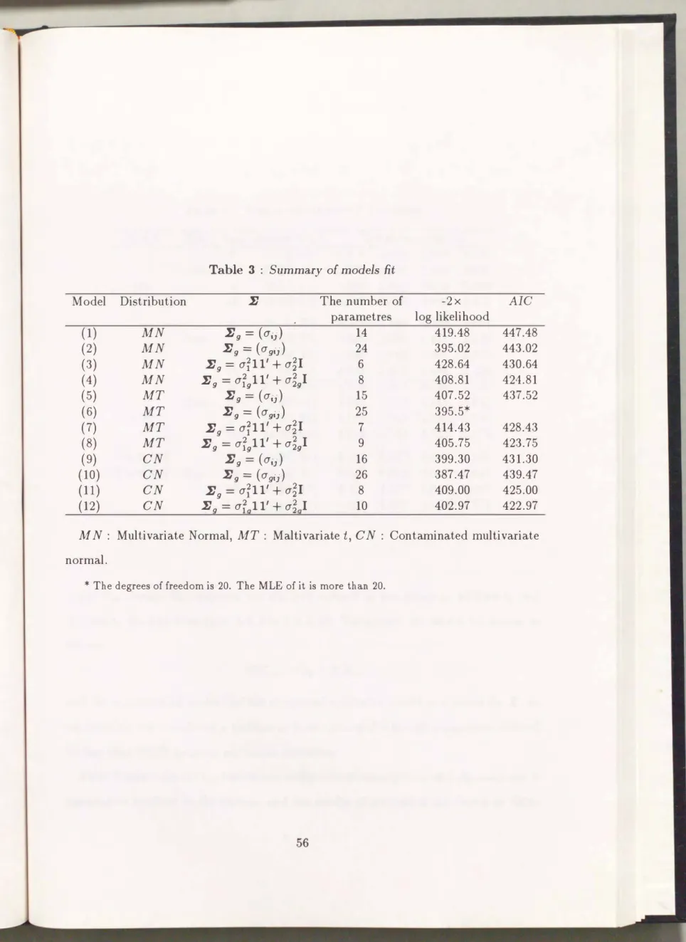
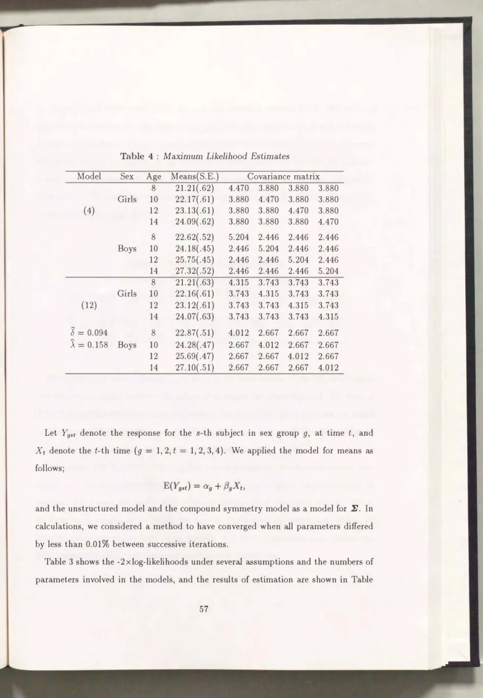
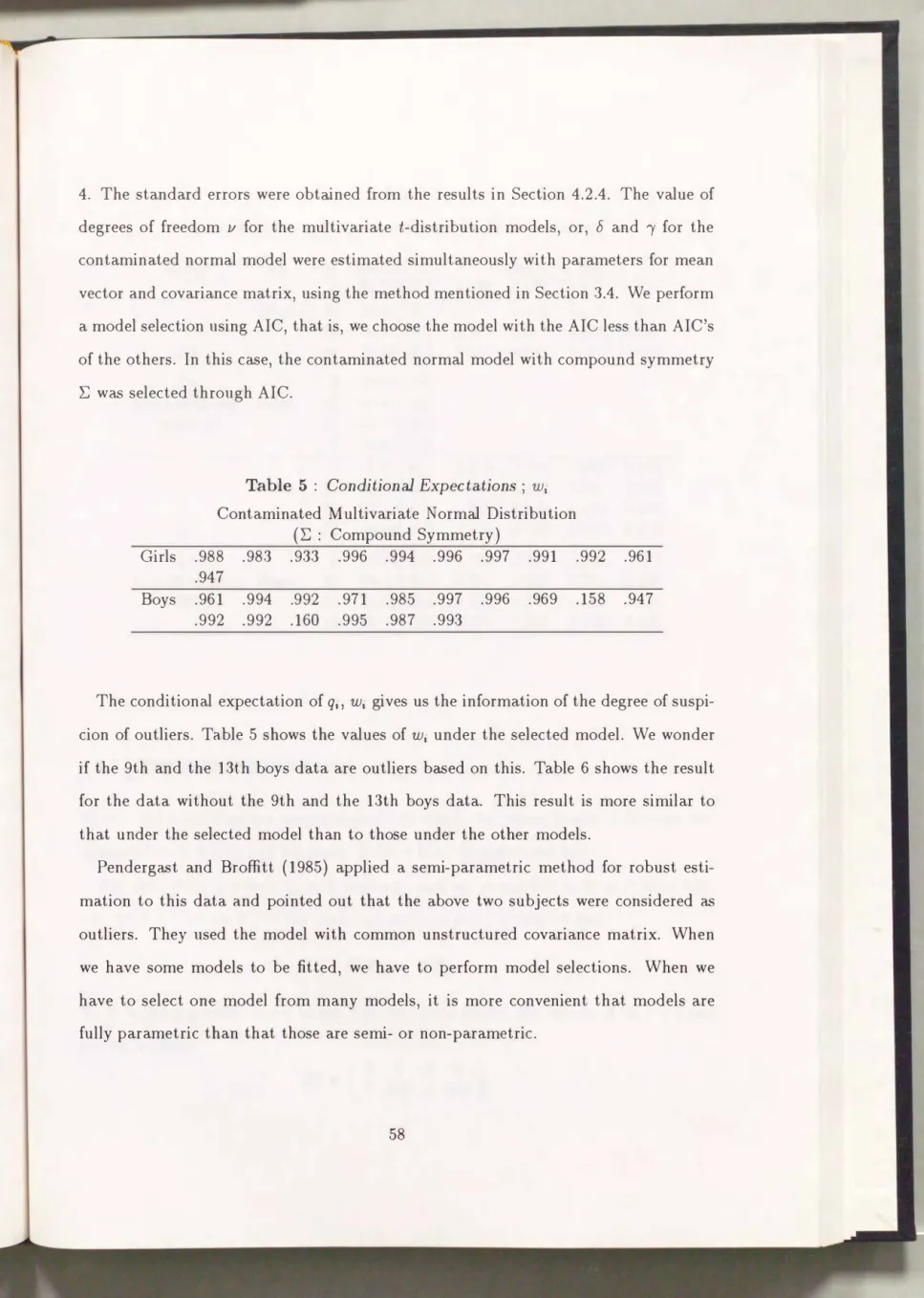
4.3 Numerical examples . . . . . 54
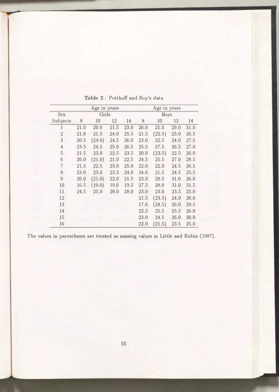
4.3.1 Potthoff and Roy's data 54
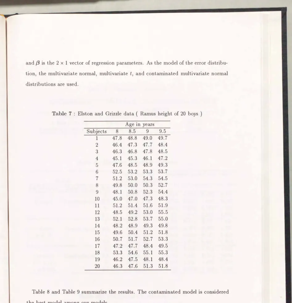
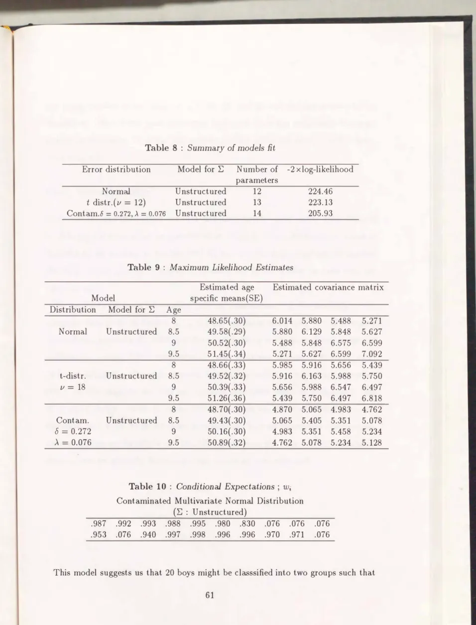
4.3.2 Elston and Grizzle's data . 59
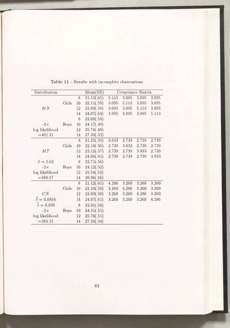
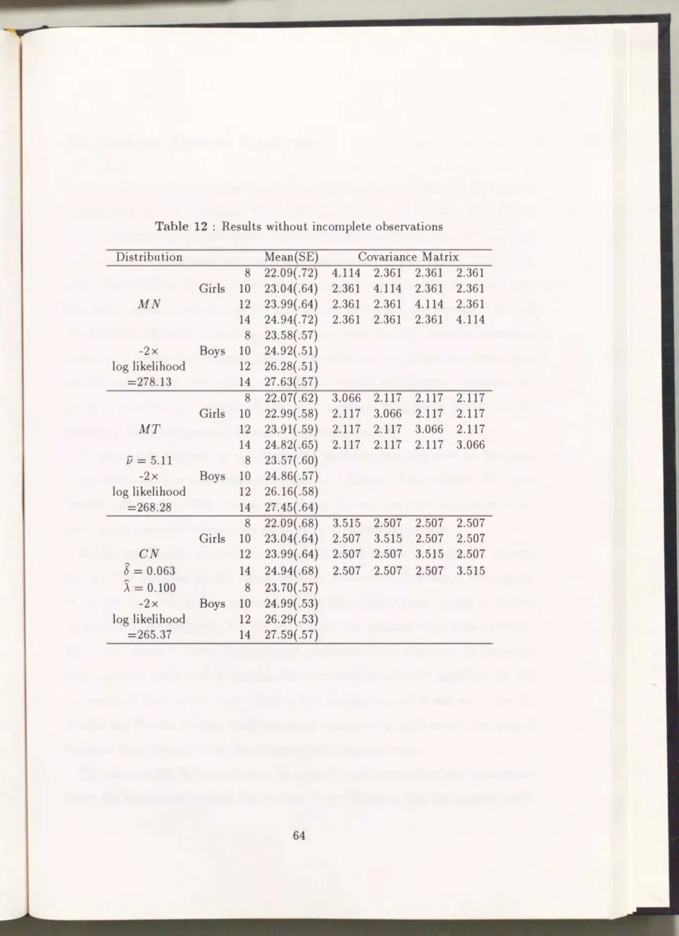
4.3.3 Incomplete data . . . . 62
5 Robust Factor Analysis 65
5.1 Robust model . . . . . 66
5.2 Estimation of the parameters 68
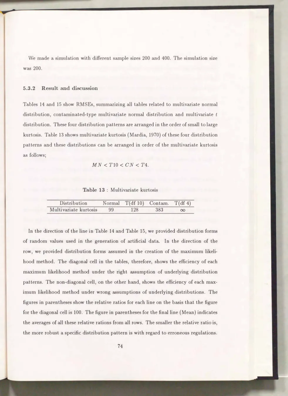
5.3 Simulation study . . . 72
5.3.1 Simulation plan 72
5.3.2 Result and discussion . 74
5.4 Application to real data 85
5.4.1 Model selection 90
5.4.2 Outliers . . . . 92
5.5 Discussion and conclusion 95
References 97
1 Introduction
Much of the classical statistical methodology in multivariate analysis is concerned with models in which the underlying observation vectors are assumed to independently follow multivariate normal distributions. We, however, are often faced to the cases that the normality assumption is not appropriate for the data. There are some typical cases the normal model dose not appear to fit. One is the case all of observations follow the same distribution but it is not normal and the other important case is that most of observations follow the normal distribution but that a few observations are generated by a different mechanism.
Observations of failure time in survival analysis can be regarded as positive random variables with asymmetric distribution. If some suitable transformations for normality can be formed, eg. the Box-Cox transformation
(
Box and Cox 1964)
, we would apply the methods for the normal model. Otherwise, it is much more difficult to derive an inference method for obtaining optimal parameter values and to examine its properties under such distribution than under the normal distribution. In this case, non-parametric or semi-parametric methods are often applied to survival data, for the sake of robustness. Among these, Cox(
1972)
's proportional hazard model may be one of the most useful semi-parametric model for survival data. As extension of Cox's to multivariate case, Yamaguchi(
1986)
considered several models for association in bivariate data with the proportional hazards assumption. Because of being semiparametric, these models include some unspecified parts treated as nuisance functions or nuisance parameters and which forces us to construct conditional inferences for objective parameters
(
see Kalbfleisch and Sprott 1970 ; Kalbfleisch and Prentice 1973; Cox 1975
)
.Another non-normal case may happen when the data include some outliers. An intuitive definition of outliers would be "observations which deviate so much from another observations as to arouse suspicions that they are generated by a different
mechanism". In the context of the presence of outliers two main problems arise. One is the detection of outliers and the other is the construction of procedures which are not heavily affected by outliers, that is, robust procedures.
Many workers empirically have pointed out that the distribution of really observed error terms often have heavier-tail than that of the normal distribution. In particular, Jeffreys
( 1961)
claimed that most error distributions could be approximated by the t distribution with 5,6
or7
degrees of freedom.Difference in the tail parts, is so influential to the results of estimation that when the normality assumption is not appropriate for given data, the t model or mixture model is often applied instead of the normal error model.
(
see Kariya and Shinha1989,
forthe robustness of statistical tests.
)
The scale mixtures of normal distributions are one of the most popular easily handled families of symmetric distributions with heavytails relative to the normal distribution, which are suitable as error distributions used instead of the normal when the data may include outliers. We might be faced to the problem of model selection, in deciding which distribution would be most appropriate.
Then we shall use AIC, the remarkably useful tool for this problem.
Many statistical significant tests for detection of outliers were proposed. Barnett and Lewis
(1978)
listed 44 tests concerned with normal distribution. In this article, however, we do not use any tests to detect outliers. The detection of outliers shall be also treated as the problems concerned with model building and model selection.The EM algorithm is introduced by Dempster et al.
(1977)
for computing maximum likelihood estimates from incomplete data. This EM algorithm is also available for pseudo incomplete data. W hen the error are assumed to follow a scale mixture of normals, we consider unobservable random variables in place of the unknown mixing parameters and treat the additional variables as missing values. One remarkable merit of use the EM algorithm is that we can handle ordinary missing values contained in the data simultaneously. Knowledge, or absence of knowledge, of the mechanisms that led to certain values being missing is a key element in choosing an appropriate analysismethod and in interpreting the results. In many cases, however, the mechanism leading to missing data does not enter explicitly; then, an assumption is being made that the mechanism is ignorable. We do not discuss the mechanism leading to missing data in detail and the missing values are assumed to be missing at random ( Rubin 1976 ; Little and Rubin 1987 ) through this article.
This article includes five Sections. Section 2 gives a detailed review of work done in Yamaguchi (1988a). We consider several semi-parametric models in survival analysis with the proportional hazards assumption. Those models include some nuisance parts which force us to estimate objective parameters by means of partial likelihood ( Cox, 1985; Wong, 1986 ). A test for the proportional hazards hypothesis is also proposed.
Section 3 deals with linear model with symmetric and heavy-tailed error distribu
tions ( Yamaguchi 1989 ). The scale mixtures of normals are used there as the error distributions, presenting a new method of maximum likelihood estimation through the contaminated normal error model (Yamaguchi 1990c ). Model selection and detection of outliers are also considered.
In Section 4, the analysis of repeated measures data is studied in the situation we have some suspicious observations as outliers (Yamaguchi 1989a, Yamaguchi 1990b ). For these data, we utilize the model given by Jennrich and Schluchter ( 1986) and the results derived in Section 3. Two numerical examples of real data are illustrated.
Section 5 gives a new robust method in factor analysis ( Watanabe and Yamaguchi 1989, Yamaguchi and Watanabe 1990a ) and demonstrates the robustness of these methods in comparison with usual normal factor analysis by a Monte Carlo simulation ( Yamaguchi and Watanabe 1990b ). Finally, model selection and detection of outliers in factor analysis are discussed with the data due to Mardia et al. (1979) as numerical example.
2 Model for Association in Bivariate Survival Data
The construction of bivariate or multivariate distribution has interested many statisti
cians from the early days. One approach is to extend a univariate distribution remain
ing its properties. The multivariate normal distribution is one of the most popular example. In survival analysis, we know the multivariate shock model introduced by Marshall and Olkin
(1967),
which is a generalization of the lack of memory property of the exponential distribution. In particular, in the bivariate case, Plackett(1965)
considered to make a class of bivariate distributions with a parameter which was a measure of association, when two marginal distributions were given.
In survival analysis, especially, analysis of the survival times of fatal patients, its main purpose is to evaluate variation of risk with respect to time and real-time control rather than prediction of survival time. From this point of view, modeling on the hazard function stands on actual meanings and needs. We also construct a model for association in bivariate survival data on the hazard function.
When we observe pairs of failure times, one of our main interests is whether one
failure affects the other failure time. This question can be answered by hazard regres
sion model analysis
(
Cox,1972, 1975),
regarding one failure times as time-dependent covariates which possibly influence the hazard for the other failures. For another approach, Clayton
(1978)
introduced a model for association in bivariate survival data with a parameter which has a simple interpretation. Lets
andt
be two survival times andf(s, t)
be its joint probability density function. Then Clayton's model satisfiesf(s, t) [" [" f(u, v)dudv =
(}{' f(u, t)du {" f(s, v)dv.
Representing by the hazard function, for any
s0, t0 (> 0), hJ(so It= to)
hJ(so It> to) = ht(to Is= so)ht(to Is> so)=
e,where
h(. I . )
denotes the conditional hazard function. Clayton applied this model to familial studies of disease incidence. Parametric and semi-parametric estimationwithin this model is discussed by Clayton
(1978)
and Oakes(1982),
although a fully satisfactory non-parametric procedure has not yet been found (Cox and Oakes,1984).
Now we consider the following case. A pair of individuals are exposed to risk at the same time and they always affect one another. In this case, a failure of the partner may change the hazard function of the remainder, without delay. Reflecting such situation, we construct models with parameters which are interpreted as same concept of odds ratio of contingency tables.
2.1 Bivariate survivor function
In the case of univariate, if one of the probability density function, cumulative dis
tribution function, survivor function, and hazard function is uniquely determined the other three functions are automatically determined. Now such relationship in bivariate case is shown.
Let
T(l), T(2)
be two positive random variable. We define the following four hazard functions.where
h(i)(t)
= lim2_
Pr(T(
i)
<t
+ �I r<l)
>t T(2)
>t)
A-+0 � -
' -
'h*<')(t I t')
=J!-To �
Pr(T(')
<t
+ f:lI r<•l � t, r<i)
=t'),
t � t',
i = 1,2,
i +j
= 3.These four functions determine the joint distribution of
T(l), T(2),
if these are continuous. The joint probability density function is, for
t(l) ::; tC2),
t(l) t(2)
f(tCI), t<2))
= exp{
-lo f [h(1)(t)
+h(2)(t)]dt- l f
t(l)h*(2)(t I tCI))dt} (1)
for
t<1)
> -t<2) '
X
h(l)( t<l))h*(2)( t<2) I t<1))'
(2)
Clearly,
T(1)
is statistical independent ofT(2),
if and only if, for anyt, t'
>0,
h*c1)(t 1 t') h*c2)(t 1 t')
Let
S( tC1), tC2))
denote the joint survivor function, then. 1 8S(tCl), tC2))
hc')(t)
=- S(t, t) otCi) I
t =t,t =t' (1) (2)2.2 Model for association
The purpose of analysis of two dimensional contingency table is to know the rela-
tionship between two qualitative variables. Measures of association are numerical assessments of the strength of the statistical dependence of two qualitative variables.
While we consider a model for association in bivariate failure times, at first we start from the standpoint of contingency tables. Divide a interval
[0,
oo)
intoq
subintervals such thatwhere
0
=t 1
<t2
< ... <t
q+1
= 00.We get a
q
xq
contingency table if we collect data in each subinterval Ij. Clayton(1974)
gave a method for analysis of two ordered categorical variables. The method assumes that for each of the( q - 1)
x( q - 1)
possible ways of collapsing the table into a 2 x 2 table the odds ratio is constant. Under this assumption, the inference about the constant odds ratio is performed. When the odds ratio is unit, this model is independent model. The unconditional maximum likelihood, conditional (partial)
likelihood and Mantel- Haenszel estimators have been studied as estimator of common
odds ratio of several
2
x2
tables. Breslow( 1981)
gave the properties of these estimators under a large sample scheme in which the number of tables increases but the possible marginal configurations remain fixed. In this situation, the unconditional maximum likelihood estimator is not consistent. The asymptotic relative efficiency of the MantelHaenszel and conditional likelihood estimators was given by Hauck
(1988).
Hauck et al.(1982)
examined small sample properties of these estimators and, Yamaguchi(1988)
derived a extended Mantel-Haenszel estimator and demonstrated the properties of these estimators.
We are analyzing continuous variables. The above method, of course, can be applied by dividing the interval
[0,
oo)
into some subintervals, but there is loss of information and the results depend on the way of construction of subintervals. We consider the limitation of the above model such that all lengths of subintervals tend to0,
as a model for continuous variables. LetPuv =
Pr(
T(l
) Elu,
T(2) EIv),
u, v= 1,
2, ... , q.Define
(
q- 1)
odds ratios for each of T(l) and T<2), respectively, as follows,i=l,2,
.
.. ,q- 1
.When all lengths of subintervals tend to zero, the limits of these odds ratios are the ratios of hazard functions. Let
Qui= L Piv,
'v=l
q
i
Ql2i = L L Puv' u=i+l v=l Q2li
=L Piv,
qv=i+l
and
then
and
q q
Q22i
=2::: 2::: Puv'
u=i+l v=i+l
Now for fixed
ti,
when�i
=ti+l
-ti
tends to zero,and
For the odds ratio,
Furthernnore, let
h**(')(t I TJl
<t)
=g� �
Pr( T ( i )
<t
+!:;,.I y(i) � t, y(J)
<t),
then
i = 1, 2, i +
j
= 3,h*•(l)(t I T(2)
<t)
=-&fwS(t, 0)
+&fwS(t, t)
S(t, 0) - S(t, t)
Therefore
Similarly,
QuiQ22i Q12iQ21i
h**(l) ( ti I T(2)
<ti) h(l)(ti)
As
e;j)
is constant for any i, we obtain the model for continuous variables such thatHowever, as it may be more convenient that a bivariate distribution is represented by
h(i)
andh*(i)
than byh(i)
andh**(i),
we would like to useh(i)
andh*(i)
for our model.lim
_!_ Pr(T(i)
<t
+ �I T(i)
>t T(j)
<t)
.6.-+0 � - '
=
lim.6.-o
X f� Pr(t � T(i)
<t
+ �'TCJ)
=t')dt' J� Pr( t � T(i), T(j)
=t')dt'
f�
lim.6.-ot Pr( t � T(i)
<t
+ �'T(j)
=t')dt' J�
Pr( t � T(i), T(j)
=t')dt'
f� h*(i)(t I t')Pr(t � T(i), T(j)
=t')dt' J� Pr(t � T(i), T(j)
=t')dt'
These equations yield that if we set for any
t
andt'
> 0then
h**(i)(t 1 r<j)
<t)
=e<i)h(i)(t),
i = 1, 2, i +j
=3.
Thus we consider
(3)
as basic model for association. Clearlye(l)
=e<2)
= 1(3)
if and only if T(I) and T(2) are mutually statistically independent. W hen both of (1(1) and (1(2) are greater than one, there exists positive association, and when both of them are less than one, there exists negative association.
We add some restrictions about to the model
(3)
in order to give simple interpretations. At first we consider the case that the bivariate distribution is symmetric. That is, for any t > 0
Model 1:
I
h<1>(t) == h(t) h ·< 1) ( t1
t ') == e h ( t) h(2)(t) == h(t) h*<2)(t1
t') == eh(t),where e is any positive constant and h(t) is any integrable positive function.
In this case, from the equations
(1),
(2), the joint probability function f(t<l), tC2)) is for tCI) � tC2)for tCl) > t<2)
where
Let
t(l) t(2)
exp{-
r
2h(u)du-r
eh(u)du}eh(t<l))h(t<2))lo l
t(l)es(tCI))l-e S(t<2))8-l f(t<l))f(t<2)),
t(2) t(l)
exp{-
r
2h(u)du-r
eh(u)du}eh(t<l))h(t<2))lo l
t(2)e S( t(I))e-1 S(t(2))1-e J( tCI)) J( t(2)),
lat
dS(t)S(t) == h(u)du and f(t) == ---.
0 &
and f x,Y, f x and Jy be the joint probability density function of X and Y, the marginal density function of X and that of Y, respectively, then
fx,y(x,y) == 2{1S(x)1-8S(y)8-1f(x)f(y),
fx(x) = 2()S(x)f(x), (4)
and
2()
jy(y) = 2
_(){S(y)9-1- S(y)}f(y).
Next in the case of asymmetric case, we assume the proportionality of two marginal hazard functions, that is
Model 2:
h(1)(t) = h(t), h(2)(t) = cxh(t).
l h*<l)(t h(1)(t) = 1 t') h(t)
= ec1) h( t) h(2)(t) = cxh(t)
h*(2)(t It')= cx()(2)h(t),
In this case, the equations
(1)
and(2)
y ield the joint probability functionf(t(l), tC2)),
for
t(l) ::; tC2)
for
t(l)
>tC2)
Similarly,
t(l) t<2)
exp{- lo f (1 + cx)h(u)du - lt(l) f cx()C2)h(u)du}
x cx()(2) h( tCl))h( t<2))
cxe<2) S( t(l))'�-ae<2) S( t(2))ae<2)_1 f ( t<l)) f( t(2))'
t(2) t<
1)exp{- lo f (1 + cx)h(u)du- ltP) f cx()(1)h(u)du}
X
a()(l) h( t(l))h( t(2))
cxe(1) S( t(l))e(l)_1 S( t(2))a-e(I) !( t(l)) !( t(2)).
fx,Y(x, y) - (1 + cx)f(x)f(y)
X
{ e<l) S(
X)a-e(l) S(y )e(1)_1 }1-6
x{a()(2)S(x)a-ae<2) S(y)aeC2)_1}<5
where
fx(x) (1 + a)S(x)a f(x), Jy(y) (1 + a)f(y)
f)(1)
X
[ { S(y )e(l)_1
-S(y )a} ]1-6 1 +a- f)(1)
X
[ afJC2)
{S( )aeC2)
-1 _S( )a }]6
1 + a - afJC2) y y '
8=
{ 1
0 if if rCl)TCl)
> <TC2) TC2)
2.3 Estimation of parameters
As there is a nuisance function
h(t)
in our models, the method for estimation is based on the partial likelihood (Cox,1975),
which is generalization of conditional and marginal likelihood. Let the data{ ( tP), t�2)),
i =1, 2, ... , n}
be arranged in ascending order of failure time as follows,and Vj and wj be the following events,
�·
: The individual(j)
fails at time t j.Wj : There is no failure in an interval
[tj_1, tj)
and an individual fails at timetj.
The probability of the event
{(Vj, �·), j
=1, 2, ... , 2n}
isII 2n
Pr(Wj1
wCj-1), vCj-1))Pr(Vj1
wCj), vU-1)), j=1where
W(j) - {W W
- 1, 2,
· · ·'
W·} J 'V (
j)
={V,1 V
'2
' · · · 'V·}
J 'and the partial likelihood
LP
isLp
=II 2n
Pr(Vj I wCi), vei-l)) j=l
Data can be also represented as Table
1
at the failure times.2.3.1 Model 1
Table 1 : Data at the failure time
t(j)
Partner Died Survival Total Type
(1)
SurvivalDied Type
(2)
SurvivalDied Total
By
(5),
the partial likelihoodLp
based on Model1
isThen the log partial likelihood
fP
isfP
logL
L:[(ctJld) n
+rf;2d))
loge -log{
r)
l.s) +r)
2.s)
+e(r?d)
+r)2d))}J.
j= l
The solution of
8fP/8()
= 0,()P
satisfies the following equation,(5)
(6)
When the observations
{(x.:, y.:), i
=1, 2, ... , n}
are given, the full likelihood Lis,n
L =
IT {2BS(x.:)1-8 S(y.:)8-1 f(xi)f(y.:)}.
i=1
Here let
Pi
=H(x.:)
andq.:
=H(y.:),
where
H(t)
is the cumulative hazard function, that isH(t)
=Ia' h(u)du.
Then the log likelihood f is
This yields
and
f logL
l::{log2 +loge- n (1- B)p.:-(e -1)q.:}.
i=1
ff- n
- 2::?=1 ( q.: -p.:)"
For the estimation of
H(t),
we can use the fact that{x.:, i
=1, 2, ... , n}
is a samplewith size
n
from the distribution with the hazard function2h(x )
, that is, we use the sample cumulative hazard function as the estimate ofH(x ),
Hn(t)
=� 2{n + 1- 1 i)'
where
L(t)
denotes sum overi, X(i) :::; t,
and{xc.:)}
is the ordere d statistics of{x.:}.
Theorem 1
... n
B e
=---
2::?=1 {Hn(Y.:)-Hn(x.:)}
is a consistent estimate of e.
Proof
where
1
L:?=l{Hn(Yi)- Hn(xi)}
Be n
=
J Hn(t)d{Fn(t)- Gn(t)}
____.
j H(t)d{F(t)- G(t)},
Fn(t)
=#{i;xi
>t}jn, Gn(t)
=#{i; Yi
>t}jn,
and
F, G
are the survivor functions of X, Y, respectively.By
( 4),
j H(t)d{F(t)- G(t)} - j H(t)�{S(t)9-1- S(t)} j(t)dt- j H(t)2BS(t)j(t)dt 2-B
2
+ e 1--
-
-1
28 2
e·
As we derived a consistent estimator
Be
ofB,
we would like to derive a two-step estimator e2 from the equation(6),
which is asymptotically equivalent to the maximum partial likelihood estimator.2.3.2 Model 2
In the case of Model
2,
by(5),
the partial likelihood LP isand
logLp
L { 2n � ld)
logeCl) + cf; 2:J)
loga+ c/j 2d)
log( aeC2))
j=1
I
( (1&) + 8c1) (1d) + c2:J) + 8c2) (2d))}
- og
rj rj arj a rj .
From this
where
8£ 2n Jld) r(ld) 8()(1)
=2::::{ �(1) - QJ . },
J=1 J
80 2n '.2&) + l2d) (2d) + ()(2) (2d) _
{. =L{a; a;
_r1 r1 },
oa j=1 a Qj
(7)
The maximum partial likelihood estimates are obtained as the solutions that the above three equations simultaneously equal to zero.
Now we would like to derive consistent estimators in the same way of Model
1.
When the observations
{(xi, Yi, b'i),
i =1,
2,.
.. , n}
are given, the full likelihood L is,Here let
n
L =
II [( 1 + a)!( Xi )f(Yi){ eCl) S( Xi)a-&(l) S(yi)8(l)_1 }1-b;
i=1
then the log likelihood f is
n
f =
i=1 2::::[(1 - b'i){log a+
log8(1) - (a- f)Cl))Pi - ( f)Cl) - 1 )qi}
and, the ML estimates are
_
C 1 )
""'n .f)C2) = n L....i=1 p, nCO)
""'n,
(q·
_p·) L....i=1;6=1
t tnCo)
a
=
_""'_ n __ .L....i=1 Pi
In this case, for the estimation of
H(t),
we can use the fact that{xi;
8 =1 }
is a sample with sizen(l)
from the distribution with the hazard functionh( x )
, that is, we use the sample cumulative hazard function as the estimate ofH(x ).
H�(t) = L
c t)(n(l) : 1- i)'
where L
C
t)
denotes sum overi, x(i) � t,
and{ x(i)}
is the ordered statistics of{xi;
8 =1}.
Using this sample cumulative hazard function, we obtain consistent estimators,--
(i)- nCo)
Be - L:i=1;6=o{H�(Yi)- H�(xi)}'
- f)�2)
=n C1)
""'nL....i=1 H*(
·)
n
x,
nCo) Ei=1;6=1 { H�(yi) - H� (xi)}' nCo)
�= --- Ei=1 H�(xi)"
Theorem 2
B�l), B�2), � are consistent estimators of t)(1), t)(2) and
a,respectively.
Proof
At first, for j = 1, 2 let
and
pCj)
andG(j)
be survivor functions ofx
and y given 8=
j, respectively.( 1) 8�1) :
1
=e0
L:i=I;a=o{H�(Yi)- H�(xi)}
n(o)
=
J H�(t)d{F�0)(t)-G�0)(t)}
J H(t)d{F(o)(t)-G0)(t)}
=
j H(t) (1 + a)8C (1)){S(t)9(1)_1-S(t)0}f(t)dt-j H(t)(1 + a)S(t)o f(t)dt 1+a-81 1 +a+ 8(1) 1
= -----:---:--- - --
( 1 + a) 8( 1) 1 + a
=
1
8(1).
(2) 8�2) :
While
1
80 -
n(o) f H�(t)d{ F�1)( t) -G�l)( t)}
-n J H�(t)dFn(t)
n(o) a
- ---+
Pr(8
=0)
= --,n 1+a
j H�(t)d{F�1)(t)-G�l)(t)}
---+
j H(t)d{F(1)(t)-G1)(t)}
J a8(2)
2)j
- H(t) 1 +a_ a8(2) {S(i)09( -1-S(i)0} f(t)dt- H(t)(1 + a)S(t)0 J(t)dt
=
=
1 +a+ a8C2) (1 + a)a8(2) 1 +a -
--1 a8(2) 1
•-j H�(t)dFn(t)
---+-j H(t)DF(t)
J H(t)(1 + a)S(t)0 f(t)dt 1
1+a
By the above equations,
(3) �:
1 1
- ----+ -
� (j(2).
1 l:i=l H�(
Xi)
ac n(o)
-n�o) ! H�(t)dFn(t)
-+
1 : a j H(t)dF(t)
1 : a j H (t)(1 + a)S(t)a f(t)dt 1+a 1
a 1 +a 1
Also in this case, we can easily obtain the two-step estimators using these consistent estimators.
By
(
7)
, the maximum partial likelihood estimators satisfy the equations""'�n Jld)
e(l) - L,J=l J
p
-
(1d)L2n j=l
r j (1 •)+8(1) (1d)+ ... (2•)+ ... 8(2) (2d) P r j r.apr
ja p
P r j_
""'2n 12d)
e(2) - L,J=l a;
P
-
r(2d)L2n j=l
r j (1•)+8(1) (1d)+ ... (2•)+ ... 8(2) (2d) P r japr
jap
P r jL2n j=l
r j (1 •)+8(1) (1d)+ ... (2•)+ ... ()(2) (2d) P r japT
ja p
P r jA single iteration from a consistent estimators produces the two-step estimators which are asymptotically equivalent to the maximum partial likelihood estimators,
2.4 Test of the proportional hazards assumption
The proportional hazard model is popular and widely available to survival analysis with censored data. The model for association in bivariate survival data is also based on the proportional hazards assumption. An important problem arising in applying these models is to assess the proportionality of the hazards. However, the analytical results are mostly discussed on the existence of the proportionality. In fact, Andersen
( 1982)
has mentioned "a number of worked examples of analyses of survival data using this model have been published, but surprisingly little attention has been paid to the problem of model checking." In view of such a necessity of model checking, we propose a test of the proportionality of the hazards.The observations from sample i
(
i=
1,2)
are(Xij, dij) j = 1, ... , ni
' whereX··-
t) -min
(
X0
·,Uij), dij = I(Xij =X�), I(·)
is the indicator function,Xi�
is the true survival time of j-individual of i-sample with a continuous distribution function Fi , andUij
is the corresponding censoring variable. We assume thatUi1
are independent identically distributed random variable with distribution functionLi
, and that the variablesUij
are independent of the variables
Xij.
Furthermore, we assume that n;
j
n ----+ r;, 0 < r; < 1, as n ----+ oo, where n ==n1 + n2• Let the cumulative hazard function ofF; be denoted by H;(t), that is Hi(t) ==
-log{1 -Fi(t)}. Also let
N;(t) ==
#{j;
Xij � t and dij == 1}
,)'i(t) ==
#j;
Xij 2:: t,y; ( t) ==
{
1 -F;( t)} {
1-
L; (t-)}.
We assume that the supports of y;(t) are [0, oo
]
.We intend to test the null hypothesis that H1(t) == ()H2(t), fort > 0 and some unknown constant ().
Now we can write the logarithm of the Cox's partial likelihood as follows,
and let
The estimator
e
is defined as the solution to the likelihood equationThe asymptotic properties of this estimator have been studied by many workers, for example Tsiatis (1981) and Wong {1986).
Furthermore let
Bn(();
t) be the product of the parameter () and the derivative ofCn(e;
t) with respect toe.
Then,This can be interpreted as the residual at the time t. The first term of left hand side is the observed number of deaths from sample 1 until time t. The second term is the corresponding expected number under the null hypothesis.
Because the parameter f) is unknown, we replace
fJ
byff
inBn
and let,It is clear by definition that
Wn(O)
=Wn(
oo)
= 0.In the next section, we propose a test by u sing
Wn(t).
2.4.1 Newly proposed test At first we give two lemmas.
Lemma 1
Under H 1 ( t)
=fJ0H 2( t) for any t
� 0and some fJ0 , the estimator ff is strongly consistent.
Proof
Bn(B; t)
is clearly a non-increasing function of e. For fixed e, as n � oo,where
-Bn(B; t)
1 ----+B(fJ; t),
a.s.,n
B(fJ;t)
=r r1Yt(s)r2Y2(s) d{Ht(s)- fJH2(s)}.
lo fJr1y1(s)
+r2y2(s)
If
H1(t)
=fJ0H2(t)
for any t � 0, thenB(fJ0;
oo)
= 0.B(fJ; t)
is also a strictly decreasing function on a neighborhood offJ0
• Therefore,Pr( lim
n-+oo 1J
=fJ0)
= 1.Let
and
G(t)
=Q(t)/Q(
oo)
.Lemma 2
Under
H1(t)
=80H2(t) for any t
> 0and some
Bo,the process {Vn(t);
0 :s;t
:s;oo} converges in law to the process {W0(G(t));O
:s;t
:s; oo}
,where W0(·) is the tied-down Brownian motion process.
Proof
See Theorem
1
of Wei(1984).
Let
This is our proposed test statistic with the properties which are represented by follow- ing two theorems.
The above two lemmas yield the following theorem.
Theorem 3
Under the null hypothesis, the asymptotic distribution of Tn is same to the distribution of
The consistent property of this test is obtained by the next theorem.
Theorem 4
When the null hypothesis is not hold, for any
c > 0,lim Pr
( T
n > c)
= 1.n-+oo
Proof
From the proof of lemma
1,
the estimatore
converges to a constant e A ' even if the assumption of proportionality of hazards is violated. On the other hand, for fixedt,
Clearly there exists some
t*
> 0 such thatTherefore,
Wn(t*)
---+ oo in probability, for somet*
and Tn ----+ oo in probability.2.4.2 Remarks
The tables of the critical points of the distribution of
f01 W0(t)2dt
were given in some papers, for example, Schumacher(1984).
A general form of the integral-type test statistics of this problem can be represented as follows,
where '1/J is a weight function. We can obtain various test statistics by selection of the weight function '1/J. For example, when the estimated variance function of
Vn(t)
is selected as
'1/J(t)-I,
the test statistic Tn,t/J is an Anderson-Darling type test statistic.The asymptotic distributions of these statistics were studied in Durbin
(1973).
3 Linear Model with Heavy-tailed Error Distri
butions
Error terms in most statistical models are assumed to be the random variables fol
lowing the normal distribution, and under this assumption, the maximum likelihood estimation is carried out. In this case, the theoretical validity of the results is guar
anteed only when data satisfy the assumption of the normality. In the general case of applying such a method to actual data, its robustness becomes a problem.
As a model of error distribution other than the normal distribution, a scale mixture of normals might be used, which has a relatively heavier tail than that of the nor
mal and is unimodal and symmetrical distribution. The family of scale mixtures of the normal distribution includes, in particular, the t-distribution, double exponential distribution and logistic distribution.
The assumption of a heavier-tailed distribution reflects interest in estimates which are relatively unaffected by outliers. In particular, the t-distribution has been fre
quently used in analysis of real data (Zellner
1976,
Sutradhar and Ali1986
and so on.), when they considered that data included some outliers. Aitkin and W ilson(1980)
treated several types of mixture models of two normals. In this section, we do not confine the t family or contaminated normal family, but instead employ the family of scale mixtures of the normals and give a general method for parameter estimation. At that time two problems would arise. One is the identification of error distribution in the family and the other is the detection of outliers. As mentioned in Chapter
1,
we treat both problems as the model selection with the help of the AIC.3.1 Linear model and iteratively reweighted least squares
We begin with the linear model and iteratively reweighted least squares (IRLS). The data consist of an n x
1
response vector Y and an n x m design matrix X. It isassumed that
Y
=Xf3
+ e,where
f3
is a vector of parameters ande
is a vector such that the components si ofa-1e
are independently and identically distributed with known density f(si)
on -oo <Si
< oo. In the context of ordinary least squares we do not use the assumption of error distribution. The weigthed least squares estimate of{3
is chosen to minimize(Y- Xf3)'W(Y- X/3), (8)
for a particular given
W,
whereW
is a positive definite diagonal matrix. We assume that X'W X is full rank, so that the unique solution which attains the minimum of(8)
exists, and it can be written
b(W)
=(X'WX)-1(X'WY).
As the weighted least squares estimate depends on the weight matrix
W,
we have to select proper weight matrix. When the weight matrix is not fixed, IRLS is used. IRLS is a process of obtaining the sequenceb(o), b(l>,
... , andb(l+l)
for l >0
is a weighted least squares estimate corresponding to a weight matrixwCl),
wherewO+l)
dependson
b(l).
To define a specific version of IRLS, we need to define a sequence of the weight matrices.A general statistical justification for IRLS arises from the fact that it can be viewed as a ML estimation.
The log likelihood is
where
Let
n
£({3, a)
= -nloga +I:
logf(si),w
(
s)
={
i=l
for s
-=/= 0
for s =
0.
(9)
(10)
We assume in (10) that
f(s)
> 0 for all s, thatd
f(s)ld
s exists for z =/= 0 and that w(s) has a finite limit as z--. 0. Also, since w(s) is selected as the weight function we must assume thatdf Ids
� 0 for s > 0 anddf Ids
� 0 for s < 0, hencef
( s) is unimodal with a mode at s = 0. Furthermore, to simplify the theory we assumedf(O)Ids
= 0.Dempster et al.(1980) gave the following Lemma and Theorem concerned with the connection between IRLS process and the log likelihood function (
9).
Lemma 3 For
({3, cr)
such that cr > 0 and w( zi)
is finite for all i, the equations derived from the log likelihood{9)
are given byX'WY - X'W X{3
= 0, (11)and
- (Y- X{3)'W(Y- X{3)
+ ncr
2 = 0, (12) whereW
is a diagonal matrix with elements w(s1), w(s2), ... , w(sn)·Lemma 3 suggests an IRLS procedure. Since
W
depends on{3
andcr,
we cannot immediately solve the equations (11), (12). Thus we might derive an iterative procedure: at each iteration substitute the temporary values of
{3
and cr into the expression forW;
then, holdingW
fixed, solve (11) and (12) to obtain the next values of{3
anda, that is, we take
(13) and
(14)
Theorem 5 If an instance of an IRLS algorithm defined by
{13)
and{14)
converged to({3*, cr*)
where the weight are all finite andcr*
> 0, then({3*, cr*)
is a stationary point of£({3,
a)
.3.2 Scale mixtures of normal distributions
If u is a standard normal random variable with density
and q is a positive random variable distributed independently of u with distribution function M( q), then the random variable
z =uq-112 is called to have a scale mixture of normal distributions. Andrew
et al.(1972) said it had a normal/independent distribution.
The scale mixtures of normal distributions are a convenient family of symmetric dis
tributions for components of error terms. The following examples show some familiar examples of these.
Example
1 :Contaminated normal distribution If M(q)
={ 1-0 � if q if q
= =1
,\otherwise
then the distribution of
zis the contaminated normal distribution with contaminated fraction o and variance inflation factor
,\,that is,
z f'J
(1- o)
xN(o, E)+ o
xN(o, E/ -\).
Example
2 : tdistribution
Let
vbe a constant. If the distribution of
v xq is x2 distribution with
vdegrees of freedom, then the distribution of
zis the
tdistribution with
vdegree of freedom.
When
v =1, it is also called the Cauchy distribution.
Example
3 :Double exponential distribution
If
1 2 ( 1 ) M(q) = 2q- exp - 2q ,
z has the double exponential distribution with the probability density function
f
( z) = 1-
2 exp(-I
zI).
Example 4 : Logistic distribution If
00 k
M(q) =
L(
-1)k-lk2q-2exp( --),k=l 2q
z has the logistic distribution with the distribution function F(z) = [1 + exp( -x
)]-1.
Dempster et al. (1980) pointed out a close connection with IRLS. Knowledge of the scale factors
qi112
in each component ei
=�uiqi112
would lead to the use of weighted least squares with weight matrix W whose diagonal elements are q1, q2, . • •,
qn, and treating these weights as missing data might lead to a statisticall y natural derivation of IRLS.The density function of
z, f(z)
is(15)
Proposition 1 Suppose that
z
is a scale mixture random variable of normal distribution with the density function (
15)
Then for 0<I
zI<
oo;(i)
the conditional distribution of q givenz
exists, (ii) E(qkI
z) < oo, fork > -1/2,(iii) w ( z) = E ( q
I
z)'(iv) dw(z)/dz = -zvar(q
I
z)
,(
v) w( z) = w(- z) is finite, positive, and nonincreasing for
z >0.
For z = 0:
(
vi) the conditional distribution of q given z exists if and only if E(q112)
< oo,(
vii) w( 0)
�w( z) for z =f. 0 and w( 0) is finite if and only if E( q312)
< oo,(
viii) dw(O)/dz is finite if and only if E(q512)
< oo.Proposition 2
Suppose that u
rvN(O, 1) and that q is a positive random variable distributed independently of u with distribution function M(q). Then
z = uq-1/2
is equivalent to that the conditional distribution of z given q = qo is N(O, 1/qo).
Proposition 3
The kurtosis of
zis never less than that of u.
Proof
E( u4q-2) E( u2q-1 )2
E( u4) E( q-2) E( u2)2E( q-1 )2
E(u4)
>
E(u2)2.
The family of scale mixtures of the normal is heavier-tailed than the normal distri
bution in the meaning of the kurtosis. We note that the condition of the normality of
u
is not necessary in the above lemma, that is, even whenu
is not limited to a normal random variable, the tail b ecomes heavier than that of the distribution of the original random variable.3.3 Multivariate model
We now consider an extension of the above results to the multivariate case.
3.3.1 Basic statistics
Let U be a p-component random vector distributed as N ( o,
:11)
and q be a positive random variable distributed independently of U with distribution function M(q). Then the random vector Z = U q-112 has a scale mixture distribution of multivariate normal.Proposition 4
The density function of
Z,f
( Z)is
The mean vector and covariance matrix of Z are reprensented by the following lemma.
Proposition 5
E(Z) =
0,
The next lemma gives the same result in the multivariate case of lemma 3. The multivariate kurtosis K2,p is defined by Mardia
(1970)
as follows:Let X be a arbitrary p-dimensional random vector, p. be its p x
1
mean vector, and:11
be its p x p covariance matrix. ThenProposition 6
The multivariate J(urtosis of
Zis not less than that of
U.Proof
Z'
1')}_1 Z )2]
=
E[(�12{E(-ZZ q q 172 q
E[( �Z'{E( �)E(ZZ')}-1 Z)2] q q
1 1
=
E[Z'{E(ZZ')}-1Z]2E(-){E(-)}-2 q2 q
>
E[Z'{E(ZZ')}-1ZY
Proposition 7
and if Z' :E-1 Z
=Z�:E-1 Zo then E(q I Z)
=E(q I Zo).
Let
s2
=s2(Z)
=Z' :E-1 Z
andw(s2)
=E(q I Z),
becausew
has the same value ifs2 is same.
Proposition 8
w( s2) is finite, positive, and nonincreasing for s2 =f
0.Proof
dw
1fooo q2(21f)-1/2q1/2 I :E �-1/2
exp(-tqs2)dM(q) ds2 2 fooo(21f)-1/2q1/2 I :E 1-1/2
exp(-tqs2)dM(q)
1
fooo q(21f)-1/2q1/2 I :E �-1/2
exp(-tqs2)dM(q) 2 +2{ fooo(21f)-1/2q1/21 :E 1-1/2 exp(-tqs2)dM(q) }
< 0
We now consider the multivariate regression to give the relation between the conditional expectation of q given
Z
and IRLS.Suppose Y
1,Y 2, ... , Y
nare a set of n observations, Yi following the model,
(17)
where {3 is a p
x mmatrix of parameters, Xi is a known design matrix and ei / CJ is a vector with the density function f( ei) and
�' =CJ21P for the sake of simplicity. Then the log likelihood function is
Let
and
np
nf(/3)
=--logCJ2
2 +L:logf(ei).
i=l
*
W··=
l)1 df( ei) e· ·J(e·) de·
l) l 'W*
i =d' 1ag will { *
wi2'*
. . ., wip' * }
(18)
where eij is the j-th component of ei. Then the likelihood equations from (18) are
n
L:w:eiX�
= o,i=l
and
n
npCJ2- L:e�w:ei
= o.i=l
Proposition 9
If ei has the density function {1 0}, then
While wi1 is a weight of the j-th component of the i-th individual, E( qi I ei) might
be regarded
asa weight of the i-th individual which is regarded
asa weighted average
3.4 ML estimation and EM algorithm
We now establish a concrete procedure of ML estimation using the EM algorithm. It is assumed that
Y i = {3X i
+ei (
i =1, .. , n),
andei
is independently identically distributed from a scale mixture of multivariate normal. Namely, there exist
n
mutually independent positive random variablesqi,
which follow the distribution function M(qi),
and conditional on
qi, ei
follows N( o,� / qi)·
According to the method of description of the EM algorithm by Dempster et al.( 1977), {Yi}
represent the directly observed data, called incomplete data because there is assumed to exist further potential data{ qi}
which are not observed, and we denote by{
0i} = {Y i, qi}
a representation of the complete data, including both observed and unobserved. The log likelihood of{
0i}
IS,
£({3, �)=Canst.-�
logI � I -� t qi(Yi-{3Xi)' �-1(Yi- {3Xi). (19)
2 2
i=l
The evaluation of the conditional expectation of £({3,
�) (19)
is realized in E-step, and the maximization of E(£I Yi)
with respect to the objective parameters is realized in M-step, respectively.E-step: W ith the observed data
Yi
and the temporary values of parameters{3(l), �(l),
the conditional expectation of £ is evaluated. In this case it is none other than determining the conditional expectation of
qi,
which would be determined if M(.) is specified.M-step: Assuming that
q?+l)
determined in the E-step was given, the estimated values of the parameters are renewed such that these values maximizes the tern- porary log likelihood. In this case,�(l+l) = i=l t q?+1)(Yi-{j(l+l) Xi)(Yi-{j(l+l) Xi)'fn.
The above E-step and M-step are repeatedly carried out, taking the proper initial values, and the ML estimation are obtained. The E-step is materialized by specifying the distribution of q. Hereinafter, its several examples are shown.
Example 5 :
Contaminated multivariate normal distribution
where ,\
<0 and 0
< 8 < 1.{
1- 8if q
=1
M( q)
= 8if q
=,\
0 otherwise
When M( q) is specified as described above, it is to assume the distribution of the mixture of
N(
o,.E) and
N(
o, -'1/,\) in the ratio of 1
- 8to
8.Hereupon, the conditional distribution of q when
Y, Xand the temporary values
----(1) --(l)
of the parameters f3 ,
-'1are given is concretely evaluated, and
is obtained, where
E(q I
e)
1- 8 + 8).1+PI2
exp{(1- ,\)
cP/2}
1- 8 + 8,\P/2
exp{(1- ,\)d2/2}
Example 6 :
Multivariate
tdistribution
(20)
If q
xv has the chi-squared distribution with v degrees of freedom, the marginal distribution is the multivariate
tdistribution (Cornish, 1954). At this time,
w(l+l) =
E(q I
e)
=