Basic Queueing Theory

Basic Queueing Theory

Dr. János Sztrik

University of Debrecen, Faculty of Informatics

Reviewers:

Dr. József Bíró

Doctor of the Hungarian Academy of Sciences, Full Professor Budapest University of Technology and Economics

Dr. Zalán Heszberger PhD, Associate Professor

Budapest University of Technology and Economics

This book is dedicated to my wife without whom this work could have been nished much earlier.

• If anything can go wrong, it will.

• If you change queues, the one you have left will start to move faster than the one you are in now.

• Your queue always goes the slowest.

• Whatever queue you join, no matter how short it looks, it will always take the longest for you to get served.

( Murphy' Laws on reliability and queueing )

Contents

Preface 7

1 Fundamental Concepts of Queueing Theory 9

1.1 Performance Measures of Queueing Systems . . . . 10

1.2 Kendall's Notation . . . . 12

1.3 Basic Relations for Birth-Death Processes . . . . 13

1.4 Optimal Design of Queueing Systems . . . . 15

1.5 Queueing Software and Collection of Problems with Solutions . . . . 17

2 Innite-Source Queueing Systems 19 2.1 The M/M/1 Queue . . . . 19

2.2 The M/M/1 Queue with Balking Customers . . . . 46

2.3 The M/M/1 Priority Queues . . . . 51

2.4 The M/M/1/K Queue, Systems with Finite Capacity . . . . 54

2.5 The M/M/∞ Queue . . . . 60

2.6 The M/M/n/n Queue, Erlang-Loss System . . . . 61

2.7 The M/M/n Queue . . . . 68

2.8 The M/M/c Non-preemptive Priority Queue (HOL) . . . . 94

2.9 The M/M/c/K Queue - Multiserver, Finite-Capacity Systems . . . . 94

2.10 The M/M/c/K Queue with Balking and Reneging . . . . 99

2.11 The M/G/1 Queue . . . 102

2.12 The M/G/1 Priority Queue . . . 114

2.13 The M/G/c Processor Sharing Queue . . . 120

2.14 The GI/M/1 Queue . . . 120

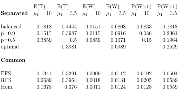
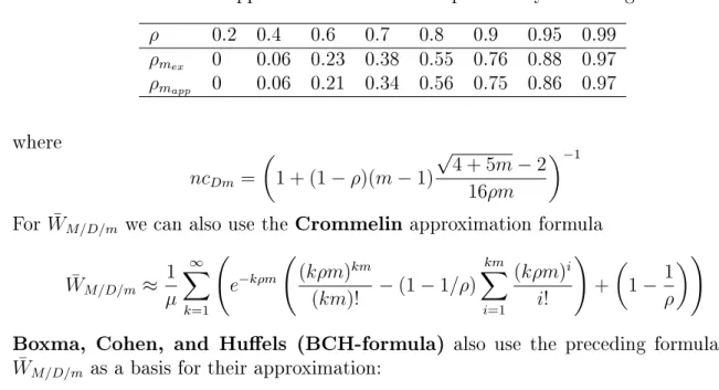
2.15 Approximations . . . 122

3 Finite-Source Systems 129 3.1 The M/M/r/r/n Queue, Engset-Loss System . . . 129

3.2 The M/M/1/n/n Queue . . . 133

3.3 The Heterogeneous M / ~ ~ M /1/n/n Queue . . . 149

3.4 The M/M/r/n/n Queue . . . 152

3.5 The M/M/r/K/n Queue . . . 165

3.6 The M/M/c/K/n Queue with Balking and Reneging . . . 169

3.7 The M/G/1/n/n/P S Queue . . . 171

3.8 The G/M/r/n/n/F IF O ~ Queue . . . 174

4 Exercises 183

4.1 Innite-Source Systems . . . 183

4.2 Finite-Source Systems . . . 200

5 Queueing Theory Formulas 203 5.1 Notations and Denitions . . . 203

5.2 Relationships between random variables . . . 205

5.3 M/M/1 Formulas . . . 206

5.4 M/M/1/K Formulas . . . 207

5.5 M/M/c Formulas . . . 208

5.6 M/M/2 Formulas . . . 210

5.7 M/M/c/c Formulas . . . 212

5.8 M/M/c/K Formulas . . . 213

5.9 M/M/ ∞ Formulas . . . 215

5.10 M/M/1/K/K Formulas . . . 216

5.11 M/G/1/K/K Formulas . . . 218

5.12 M/M/c/K/K Formulas . . . 219

5.13 D/D/c/K/K Formulas . . . 221

5.14 M/G/1 Formulas . . . 222

5.15 GI/M/1 Formulas . . . 231

5.16 GI/M/c Formulas . . . 233

5.17 M/G/1 Priority queueing system . . . 235

5.18 M/G/c Processor Sharing system . . . 243

5.19 M/M/c Priority system . . . 244

Appendix 245

Bibliography 246

Preface

Modern information technologies require innovations that are based on modeling, ana- lyzing, designing and nally implementing new systems. The whole developing process assumes a well-organized team work of experts including engineers, computer scientists, mathematicians, physicist just to mention some of them. Modern infocommunication networks are one of the most complex systems where the reliability and eciency of the components play a very important role. For the better understanding of the dynamic behavior of the involved processes one have to deal with constructions of mathematical models which describe the stochastic service of randomly arriving requests. Queueing Theory is one of the most commonly used mathematical tool for the performance evalu- ation of such systems.

The aim of the book is to present the basic methods, approaches mainly in a Markovian level for the analysis of not too complicated systems. The main purpose is to understand how models could be constructed and how to analyze them. It is assumed the reader has been exposed to a rst course in probability theory, however in the text I give a refresher and state the most important principles I need later on. My intention is to show what is behind the formulas and how we can derive formulas. It is also essential to know which kind of questions are reasonable and then how to answer them.

My experience and advice are that if it is possible solve the same problem in dierent ways and compare the results. Sometimes very nice closed-form, analytic solutions are obtained but the main problem is that we cannot compute them for higher values of the involved variables. In this case the algorithmic or asymptotic approaches could be very useful. My intention is to nd the balance between the mathematical and practitioner needs. I feel that a satisfactory middle ground has been established for understanding and applying these tools to practical systems. I hope that after understanding this book the reader will be able to create his owns formulas if needed.

It should be underlined that most of the models are based on the assumption that the involved random variables are exponentially distributed and independent of each other.

We must confess that this assumption is articial since in practice the exponential distri-

bution is not so frequent. However, the mathematical models based on the memoryless

property of the exponential distribution greatly simplies the solution methods resulting

in computable formulas. By using these relatively simple formulas one can easily foresee

the eect of a given parameter on the performance measure and hence the trends can be

forecast. Clearly, instead of the exponential distribution one can use other distributions

but in that case the mathematical models will be much more complicated. The analytic

results can help us in checking the results obtained by stochastic simulation. This ap- proach is quite general when analytic expressions cannot be expected. In this case not only the model construction but also the statistical analysis of the output is important.

The primary purpose of the book is to show how to create simple models for practical problems that is why the general theory of stochastic processes is omitted. It uses only the most important concepts and sometimes states theorem without proofs, but each time the related references are cited.

I must confess that the style of the following books greatly inuenced me, even if they are in dierent level and more comprehensive than this material: Allen [3], Gross, Shortle, Thompson and Harris [40], Harchol-Balter [46], Jain [55], Kleinrock [62], Kobayashi and Mark [65], Medhi [75], Nelson [77], Stewart [97], Tijms [117], Trivedi [120].

This book is intended not only for students of computer science, engineering, operation research, mathematics but also those who study at business, management and planning departments, too. It covers more than one semester and has been tested by graduate students at Debrecen University over the years. It gives a very detailed analysis of the involved queueing systems by giving density function, distribution function, generating function, Laplace-transform, respectively. Furthermore, a software package called QSA (Queueing Systems Assistance) developed in 2021 is provided to calculate and visualize the main performance measures. In addition, it helps to minimize a quite general mean total cost per unit time with linear objective function. The main advantage that these scripts can be run in all modern devices including smart phones, too, thus the application is very convenient for students and improve the eciency of a teacher.

I have attempted to provide examples for the better understanding and a collection of exercises with detailed solution helps the reader in deepening her/his knowledge. I am convinced that the book covers the basic topics in stochastic modeling of practical problems and it supports students in all over the world.

I am indebted to Professors József Bíró and Zalán Heszberger for their review, com- ments and suggestions which greatly improved the quality of the book. I am also very grateful to Tamás Török, Zoltán Nagy, Ferenc Veres, and Hamza Nemouchi for their help in LaTex editing.

All comments and suggestions are welcome at:

mailto:[email protected] http://irh.inf.unideb.hu/~jsztrik Debrecen, 2012, 2021

János Sztrik

Chapter 1

Fundamental Concepts of Queueing Theory

Queueing theory deals with one of the most unpleasant experiences of life, waiting. Queue- ing is quite common in many elds, for example, in telephone exchange, in a supermarket, at a petrol station, at computer systems, etc. I have mentioned the telephone exchange rst because the rst problems of queueing theory was raised by calls and Erlang was the rst who treated congestion problems in the beginning of 20th century, see Erlang [29,30].

His works inspired engineers, mathematicians to deal with queueing problems using probabilistic methods. Queueing theory became a eld of applied probability and many of its results have been used in operations research, computer science, telecommunication, trac engineering, reliability theory, just to mention some. It should be emphasized that is a living branch of science where the experts publish a lot of papers and books. The easiest way is to verify this statement one should use the Google Scholar for queueing related items. A Queueing Theory Homepage has been created where readers are informed about relevant sources, for example books, softwares, conferences, journals, etc. I highly recommend to visit it at

http://web2.uwindsor.ca/math/hlynka/queue.html

There is only a few books and lectures notes published in Hungarian language, I would mention the work of Györ and Páli [41], Jereb and Telek [57], Kleinrock [62], Lakatos and Szeidl , Telek [69] and Sztrik [104107]. However, it should be noted that the Hun- garian engineers and mathematicians have eectively contributed to the research and applications. First of all we have to mention Lajos Takács who wrote his pioneer and famous book about queueing theory [114]. Other researchers are J. Tomkó, M. Arató, L. Györ, A. Benczúr, L. Lakatos, L. Szeidl, L. Jereb, M. Telek, J. Bíró, T. Do, and J.

Sztrik. The Library of Faculty of Informatics, University of Debrecen, Hungary oer a valuable collection of queueing and performance modeling related books in English, and Russian, too. Please visit:

https://irh.inf.unideb.hu/user/jsztrik/education/05/3f.html

I may draw your attention to the books of Takagi [111113] where a rich collection of

references is provided.

1.1 Performance Measures of Queueing Systems

To characterize a queueing system we have to identify the probabilistic properties of the incoming ow of requests, service times and service disciplines. The arrival process can be characterized by the distribution of the interarrival times of the customers, denoted by A(t) , that is

A(t) = P ( interarrival time < t).

In queueing theory these interarrival times are usually assumed to be independent and identically distributed random variables. The other random variable is the service time, sometimes it is called service request, work. Its distribution function is denoted by B(x) , that is

B(x) = P ( service time < x).

The service times, and interarrival times are commonly supposed to be independent random variables.

The structure of service and service discipline tell us the number of servers, the capacity of the system, that is the maximum number of customers staying in the system including the ones being under service. The service discipline determines the rule according to the next customer is selected. The most commonly used laws are

• FIFO - First In First Out: who comes earlier leaves earlier, FCFS - First Come First Served

• LIFO - Last Come First Out: who comes later leaves earlier, LCFS - Last Come First Served

• RS - Random Service: the customer is selected randomly, SIRO - Service In Random Order

• Priority without Preemption or Head of Line (HOL), Priority with Preemption / Resume or Repeat

• PS - Processor Sharing

The aim of all investigations in queueing theory is to get the main performance measures of the system which are the probabilistic properties ( distribution function, density function, mean, variance ) of the following random variables: number of customers in the system, number of waiting customers, utilization of the server/s, response time of a customer, waiting time of a customer, idle time of the server, busy time of a server. Of course, the answers heavily depends on the assumptions concerning the distribution of interarrival times, service times, number of servers, capacity and service discipline. It is quite rare, except for elementary or Markovian systems, that the distributions can be computed.

Usually their mean or transforms can be calculated.

For simplicity consider rst a single-server system Let % , called trac intensity, be dened as

% = mean service time

mean interarrival time .

Assuming an innity population system with arrival intensity λ , which is reciprocal of the mean interarrival time, and let the mean service denote by 1/µ . Then we have

% = arrival intensity ∗ mean service time = λ µ .

If % > 1 then the systems is overloaded since the requests arrive faster than as the are served. It shows that more server are needed.

Let χ(A) denote the characteristic function of event A , that is χ(A) =

( 1 , if A occurs, 0 , if A does not ,

furthermore let N (t) = 0 denote the event that at time T the server is idle, that is no customer in the system. Then the utilization of the server during time T is dened by

1 T

T

Z

0

χ (N (t) 6= 0) dt ,

where T is a long interval of time. As T → ∞ we get the utilization of the server denoted by U _s and the following relations holds with probability 1

U s = lim

T →∞

1 T

T

Z

0

χ (N(t) 6= 0) dt = 1 − P 0 = Eδ Eδ + Ei ,

where P ₀ is the steady-state probability that the server is idle Eδ , Ei denote the mean busy period, mean idle period of the server, respectively.

This formula is a special case of the relationship valid for continuous-time Markov chains and proved in Tomkó [119].

Theorem 1 Let X(t) be an ergodic Markov chain, and A is a subset of its state space.

Then with probability 1

T lim →∞

1 T

Z T 0

χ(X(t) ∈ A)dt

= X

i∈A

P _i = m(A) m(A) + m(A) ,

where m(A) and m(A) denote the mean sojourn time of the chain in A and A during a cycle,respectively. The ergodic ( stationary, steady-state ) distribution of X(t) is denoted by P i .

In an m -server system the mean number of arrivals to a given server during time T is λT /m given that the arrivals are uniformly distributed over the servers. Thus the utilization of a given server is

U _s = λ

mµ .

The other important measure of the system is the throughput of the system which is dened as the mean number of requests serviced during a time unit. In an m -server system the mean number of completed services is m%µ and thus

throughput = mU _s µ = .

However, if we consider now the customers for a tagged customer the waiting and response times are more important than the measures dened above. Let us dene by W j , T j the waiting, response time of the j th customer, respectively. Clearly the waiting time is the time a customer spends in the queue waiting for service, and response time is the time a customer spends in the system, that is

T j = W j + S j ,

where S _j denotes its service time. Of course, W _j and T _j are random variables and their mean, denoted by W _j and T _j , are appropriate for measuring the eciency of the system.

It is not easy in general to obtain their distribution function.

Other characteristic of the system is the queue length, and the number of customers in the system. Let the random variables Q(t) , N (t) denote the number of customers in the queue, in the system at time t , respectively. Clearly, in an m -server system we have

Q(t) = max{0, N (t) − m}.

The primary aim is to get their distributions, but it is not always possible, many times we have only their mean values or their generating function.

1.2 Kendall's Notation

Before starting the investigations of elementary queueing systems let us introduce a no- tation originated by Kendall to describe a queueing system.

Let us denote a system by

A / B / m / K / n/ D, where

A : distribution function of the interarrival times, B : distribution function of the service times, m : number of servers,

K : capacity of the system, the maximum number of customers in the system including the one being serviced,

n : population size, number of sources of customers,

D : service discipline.

Exponentially distributed random variables are notated by M , meaning Markovian or memoryless. Furthermore, if the population size and the capacity is innite, the service discipline is FIFO, then they are omitted.

Hence M/M/1 denotes a system with Poisson arrivals, exponentially distributed service times and a single server. M/G/m denotes an m -server system with Poisson arrivals and generally distributed service times. M/M/r/K/n stands for a system where the customers arrive from a nite-source with n elements where they stay for an exponentially distributed time, the service times are exponentially distributed, the service is carried out according to the request's arrival by r severs, and the system capacity is K .

David G. Kendall, 1918-2007

1.3 Basic Relations for Birth-Death Processes

Since birth-death processes play a very important role in modeling elementary queueing systems let us consider some useful relationships for them. Clearly, arrivals mean birth and services mean death.

As we have seen earlier the steady-state distribution for birth-death processes can be obtained in a very nice closed-form, that is

(1.1) P i = λ ₀ · · · λ _i−1

µ ₁ · · · µ _i P 0 , i = 1, 2, · · · , P 0 −1

= 1 +

∞

X

i=1

λ ₀ · · · λ _i−1

µ ₁ · · · µ _i .

Let us consider the distributions at the moments of arrivals, departures, respectively, because we shall use them later on.

Let N _a , N _d denote the state of the process at the instant of births, deaths, respectively, and let Π _k = P (N _a = k), D _k = P (N _d = k), k = 0, 1, 2, . . . stand for their distributions.

By applying the Bayes's theorem it is easy to see that

(1.2) Π _k = lim

h→0

(λ _k h + o(h))P _k P ∞

j=0 (λ _j h + o(h))P _j = λ _k P _k P ∞

j=0 λ _j P _j . Similarly

(1.3) D _k = lim

h→0

(µ k+1 h + o(h))P k+1

P ∞

j=1 (µ _j h + o(h))P _j = µ k+1 P k+1

P ∞

j=1 µ _j P _j . Since P _k+1 = λ k

µ _k+1 P _k , k = 0, 1, . . . , thus

(1.4) D _k = λ _k P _k

P ∞

i=0 λ _i P _i = Π _k , k = 0, 1, . . . .

In words, the above relation states that the steady-state distributions at the moments of births and deaths are the same. It should be underlined, that it does not mean that it is equal to the steady-state distribution at a random point as we will see later on.

Further essential observation is that in steady-state the mean birth rate is equal to the mean death rate. This can be seen as follows

(1.5) λ =

∞

X

i=0

λ _i P _i =

∞

X

i=0

µ _i+1 P _i+1 =

∞

X

k=1

µ _k P _k = µ.

1.4 Optimal Design of Queueing Systems

The ultimate goal of the modeling is to make optimal decision on a given problem.

Queueing theory may help to do that. After obtaining the corresponding formulas one can make the decision. Like the descriptive models in classical queueing theory, optimal design models may be classied according to such parameters as the arrival rate(s), the service rate(s), number of servers, the interarrival time and service time distributions, and the queue discipline(s). In addition, the queueing system under study may be a network with several facilities and/or classes of customers, in which case the nature of the ows of the classes among the various facilities must also be specied. What distinguishes an optimal design model from a traditional descriptive model is the fact that some of the parameters are subject to decision and that this decision is made with explicit attention to economic considerations, with the preferences of the decision maker(s) as a guiding principle. The basic distinctive components of a design model are thus:

• the decision variables

• benets/rewards and costs

• the objective function

Decision variables may include, for example, the arrival rates, the service rates, number of servers, and the queue disciplines at the various service facilities. Typical benets and costs include rewards to the customers from being served, waiting costs incurred by the customers while waiting for service, and costs to the facilities for providing the service. These benets and costs may be brought together in an objective function, which quanties the implicit trade-os. For example, increasing the service rate will result in less time spent by the customers waiting (and thus a lower waiting cost), but a higher service cost. Each time we dealt with a linear cost/reward structure, in which the objective is to minimize the expected total cost per unit time in steady state. The objective function is calculated and illustrated without any details. In a design problem, the values of the decision variables, once chosen, cannot vary with time nor in response to changes in the state of the system (e.g., the number of customers present). The decision is made with respect to only one variable.

Let us introduce the following costs and benets/rewards

• CS - cost of service per server per unit time

• CWS - cost of waiting in the system per customer per unit time

• CI - cost of idleness per server per unit time

• CSR - cost of service rate per server per unit time

• CLC - cost of loss per customer per unit time

• R - reward per entering customer per unit time

Our aim is to minimize the following expected total cost per unit time with objective function

E(T otal cost) = (number of servers) ∗ CS

+ E(number of customers in the system) ∗ CW

+ E(number of idle servers) ∗ CI + (number of servers) ∗ CSR + E(arrival rate) ∗ P (loss/blocking) ∗ CLC

− E(arrival rate)(1 − P (loss/blocking) ∗ R.

It is quite a general cost function and it is calculated numerically by giving the respective costs. Depending on the decision parameter this function is illustrated and the user can determine the optimal value of the parameter and the expected total cost.

There are several books on this type of decision making using queueing formulas. In

the past years I found the following sources are very useful, Bhat [9], Gross et. al. [40],

Harchol-Balter [46], Hillier and Lieberman [51], Kobayashi and Mark [65], Kulkarni [68],

Stidham [98], White [126] in which not only the topic is treated but dierent software

tools support the decision, for example MATLAB, Mathematica, Excel.

1.5 Queueing Software and Collection of Problems with Solutions

To solve practical problems the rst step is to identify the appropriate queueing system and then to calculate the performance measures. Of course the level of modeling heavily depends on the assumptions. It is recommended to start with a simple system and then if the results do not t to the problem continue with a more complicated one. Various software packages help the interested readers in dierent level. The following links worth a visit

http://web2.uwindsor.ca/math/hlynka/qsoft.html

I highly recommend an Excel-based software package called QTSPlus to calculate the main performance measures of basic models. It is associated to the book of Gross, Shortle, Thompson and Harris [40] and can be downloaded here

http://mason.gmu.edu/~jshortle/fqt5th.html, http://mason.gmu.edu/~jshortle/QtsPlus-4-0.zip

ftp://ftp.wiley.com/public/sci_tech_med/queueing_theory/

For practical oriented teaching courses we have also developed a software package called QSA (Queueing Systems Assistance) to calculate and visualize the performance mea- sures together with optimal decisions not only for elementary but more advanced queueing systems as well. It is available at

https://qsa.inf.unideb.hu The main advantages of QSA over QTSPlus are the following

• It runs on desktops, laptops, smartphones (due to Java)

• It calculates not only the mean but the variance of the corresponding random variables

• It gives the distribution function of the waiting/response times (if possible)

• It visualizes all the main performance measures

• It graphically supports the decision making

Besides the package I have established a Collection of Problems with Solutions teaching material in which the problems deliberately listed in random order imitating the practical needs. The material can be downloaded here:

https://irh.inf.unideb.hu/~jsztrik/education/16/Queueing_Problems_

Solutions_2021_Sztrik.pdf

QSA Welcome page

M/M/1 System

If the already existing systems are not suitable for your problem then you have to create your own queueing system and then the creation starts and the primary aim of the present book is to help this process.

For further readings the interested reader is referred to the following books: Allen [3], Bose [14], Cooper [23], Daigle [25], Gnedenko and Kovalenko [39], Gross, Shortle, Thomp- son and Harris [40], Harchol-Balter [46], Jain [55], Kleinrock [62], Kobayashi [64, 65], Kulkarni [68], Medhi [75], Nelson [77], Stewart [97], Sztrik [104], Takagi [111113], Ti- jms [117], Trivedi [120].

The present book has used some parts of Adan and Reising [1], Allen [3], Daigle [25],

Gross and Harris [40], Harchol-Balter [46], Kleinrock [62], Kobayashi [65], Sztrik [104],

Tijms [117], Trivedi [120].

Chapter 2

Innite-Source Queueing Systems

Queueing systems can be classied according to the cardinality of their sources, namely nite-source and innite-source models. In nite-source models the arrival intensity of the request depends on the state of the system which makes the calculations more com- plicated. In the case of innite-source models, the arrivals are independent of the number of customers in the system resulting a mathematically tractable model. In queueing net- works each node is a queueing system which can be connected to each other in various way. The main aim of this chapter is to know how these nodes operate.

2.1 The M/M/1 Queue

An M/M/1 queueing system is the simplest non-trivial queue where the requests arrive according to a Poisson process with rate λ , that is the interarrival times are independent, exponentially distributed random variables with parameter λ . The service times are also assumed to be independent and exponentially distributed with parameter µ . Further- more, all the involved random variables are supposed to be independent of each other.

Let N (t) denote the number of customers in the system at time t and we shall say that the system is at state k if N (t) = k . Since all the involved random variables are exponentially distributed, consequently they have the memoryless property, N (t) is a continuous-time Markov chain with state space 0, 1, · · · .

In the next step let us investigate the transition probabilities during time h . It is easy to see that

P _k,k+1 (h) = (λh + o(h)) (1 − (µh + o(h)) + +

∞

X

k=2

(λh + o(h)) ^k (µh + o(h)) ^k−1 , k = 0, 1, 2, ...

By using the independence assumption the rst term is the probability that during h

one customer has arrived and no service has been nished. The summation term is the

probability that during h at least 2 customers has arrived and at the same time at least 1

has been serviced. It is not dicult to verify the second term is o(h) due to the property of the Poisson process. Thus

P _k,k+1 (h) = λh + o(h).

Similarly, the transition probability from state k into state k − 1 during h can be written as

P k,k−1 (h) = (µh + o(h)) (1 − (λh + o(h)) + +

∞

X

k=2

(λh + o(h)) ^k−1 (µh + o(h)) ^k

= µh + o(h).

Furthermore, for non-neighboring states we have

P _k,j = o(h), | k − j |≥ 2.

In summary, the introduced random process N(t) is a birth-death process with rates λ k = λ, k = 0, 1, 2, ..., µ k = µ, k = 1, 2, 3....

That is all the birth rates are λ , and all the death rates are µ .

As we notated the system capacity is innite and the service discipline is FIFO.

To get the steady-state distribution let us substitute these rates into formula (1.1) ob- tained for general birth-death processes. Thus we obtain

P k = P 0 k−1

Y

i=0

λ µ = P 0

λ µ

k

, k ≥ 0.

By using the normalization condition we can see that this geometric sum is convergent i λ/µ < 1 and

P ₀ = 1 +

∞

X

k=1

λ µ

k ! −1

= 1 − λ

µ = 1 − % where % = ^λ _µ . Thus

P _k = (1 − %)% ^k , k = 0, 1, 2, ...,

which is a modied geometric distribution with success parameter 1 − % . In the following we calculate the the main performance measures of the system

• Mean number of customers in the system N =

∞

X

k=0

kP k = (1 − %)%

∞

X

k=1

k% ^k−1 =

= (1 − %)%

∞

X

k=1

d% ^k

d% = (1 − %)% d d%

1 1 − %

= %

1 − % . Variance

V ar(N ) =

∞

X

k=0

(k − N ) ² P _k =

∞

X

k=0

k − % 1 − %

2

P _k

=

∞

X

k=0

k ² P _k + %

1 − % 2

−

∞

X

k=0

2k % 1 − % P _k

=

∞

X

k=0

k(k − 1)P _k + % ²

(1 − %) ² + % 1 − % − 2

% 1 − %

2

= (1 − %)% ² d ² d% ²

∞

X

k=0

% ^k + % 1 − % −

% 1 − %

2

= 2% ²

(1 − %) ² + % 1 − % −

% 1 − %

2

= %

(1 − %) ² .

• Mean number of waiting customers, mean queue length Q =

∞

X

k=1

(k − 1)P _k =

∞

X

k=1

kP _k −

∞

X

k=1

P _k = N − (1 − P ₀ ) = N − % = % ² 1 − % . Variance

V ar(Q) =

∞

X

k=1

(k − 1) ² P _k − Q ² = % ² (1 + % − % ² ) (1 − %) ² .

• Server utilization

U _s = 1 − P ₀ = λ µ = %.

By using Theorem 1 it is easy to see that P ₀ =

1 λ 1

λ + Eδ ,

where Eδ a is the mean busy period length of the server, _λ ¹ is the mean idle time of the server. Since the server is idle until a new request arrives which is exponentially distributed with parameter λ . Hence

1 − % =

1 λ 1

λ + Eδ , and thus

Eδ = 1 λ

%

1 − % = 1

λ N = 1

µ − λ .

In the next few lines we show how this performance measure can be obtained in a dierent way.

To do so we need the following notations.

Let E (ν _A ) , E (ν _D ) denote the mean number of customers that have arrived, departed during the mean busy period of the server, respectively. Furthermore, let E (ν _S ) denote the mean number of customers that have arrived during a mean service time. Clearly

E (ν _D ) = E (δ)µ, E (ν _S ) = λ

µ , E (ν _A ) = E (δ)λ, E (ν _A ) + 1 = E (ν _D ), and thus after substitution we get

E (δ) = 1 µ − λ . Consequently

E (ν _D ) = E (δ)µ = 1 1 − % E (ν A ) = E (ν S ) E (ν D ) = λ

µ 1

1 − % = % 1 − % E (ν _A ) = E (δ)λ = %

1 − % .

• Distribution of the response time of a customer

Before investigating the response we show that in any queueing system where the arrivals are Poisson distributed

P _k (t) = Π _k (t),

where P k (t) denotes the probability that at time t the system is a in state k , and Π _k (t) denotes the probability that an arriving customers nd the system in state k at time t . Let

A(t, t + ∆t)

denote the event that an arrival occurs in the interval (t, t + ∆t) . Then Π _k (t) := lim

∆t→0 P (N (t) = k|A(t, t + ∆t)) , Applying the denition of the conditional probability we have

Π _k (t) = lim

∆t→0

P (N (t) = k , A(t, t + ∆t))

P (A(t, t + ∆t)) =

= lim

∆t→0

P (A(t, t + ∆t)|N (t) = k) P (N (t) = k) P (A(t, t + ∆t)) .

However, in the case of a Poisson process event A(t, t + ∆t) does not depends on the number of customers in the system at time t and even the time t is irrespective thus we obtain

P (A(t, t + ∆t)|N (t) = k) = P (A(t, t + ∆t)) , hence for birth-death processes we have

Π _k (t) = P (N (t) = k) .

That is the probability that an arriving customer nd the system in state k is equal to the probability that the system is in state k .

In stationary case applying formula (1.2) with substitutions λ _i = λ, i = 0, 1, . . . we have the same result.

If a customer arrives it nds the server idle with probability P 0 hence the waiting time is 0 . Assume, upon arrival a tagged customer, the system is in state n . This means that the request has to wait until the residual service time of the customer being serviced plus the service times of the customers in the queue. As we assumed the service is carried out according to the arrivals of the requests. Since the ser- vice times are exponentially distributed the remaining service time has the same distribution as the original service time. Hence the waiting time of the tagged cus- tomer is Erlang distributed with parameters (n, µ) and the response time is Erlang distributed with (n + 1, µ) . Just to remind you the density function of an Erlang distribution with parameters (n, µ) is

f _n (x) = µ(µx) ⁿ⁻¹

(n − 1)! e ^−µx , x ≥ 0.

Hence applying the theorem of total probability for the density function of the response time we have

f _T (x) =

∞

X

n=0

(1 − %)% ⁿ (µx) ⁿ

n! µe ^−µx = µ(1 − %)e ^−µx

∞

X

n=0

(%µx) ⁿ n! =

= µ(1 − %)e ^{−µ(1−%)x} . Its distribution function is

F _T (x) = 1 − e ^{−µ(1−%)x} .

That is the response time is exponentially distributed with parameter µ(1 − %) = µ − λ .

Hence the expectation and variance of the response time are

T = 1

µ(1 − %) , V ar(T ) = ( 1

µ(1 − %) ) ² .

Furthermore

T = 1

µ(1 − %) = 1

µ − λ = Eδ.

• Distribution of the waiting time

Let f _W (x) denote the density function of the waiting time. Similarly to the above considerations for x > 0 we have

f _W (x) =

∞

X

n=1

(µx) ⁿ⁻¹

(n − 1)! µe ^−µx % ⁿ (1 − %) = (1 − %)%µ

∞

X

k=0

(µx%) ^k

k! e ^−µx =

= (1 − %)%µe ^{−µ(1−%)x} .

Thus f _W (0) = 1 − %, if x = 0,

f _W (x) = %(1 − %)µe ^{−µ(1−%)x} , if x > 0.

Hence

F _W (x) = 1 − % + % 1 − e ^{−µ(1−%)x}

= 1 − %e ^{−µ(1−%)x} . The mean waiting time is

W =

∞

Z

0

xf _W (x)dx = %

µ(1 − %) = %Eδ = N 1 µ . Since T = W + S , in addition W and S are independent we get

V ar(T ) = 1

(µ(1 − ρ)) ² = V ar(W ) + 1 µ ² , thus

V ar(W ) = 1

(µ(1 − ρ)) ² − 1

µ ² = 2ρ − ρ ²

(µ(1 − ρ)) ² = ρ 2

(µ(1 − ρ)) ² − ρ ² (µ(1 − ρ)) ² , that is exactly E (W ² ) − ( E W ) ² .

Notice that

(2.1) λT = λ 1

µ(1 − %) = %

1 − % = N . Furthermore

(2.2) λW = λ %

µ(1 − %) = % ²

1 − % = Q.

Relations (2.1), (2.2) are called Little formulas or Little theorem, or Little

law which remain valid under more general conditions.

Figure 2.1: John Little, 1928-

It should be noted that in many applications we are dealing with a required service denoted by S R , which does not mean service time. In these cases we involve some kind of capacity (speed, bandwidth) denoted by C . In that case S _R = CS and E(S) = E(R _S )/C.

It is easy to see if the required service is exponentially distributed with parameter µ than the service time is also exponentially distributed with parameter µC . That is

P (S < t) = P (S _R /C < t) = P (S _R < Ct) = 1 − e ^−µCt .

For example, router A sends 8 packets per second, on the average, to router B. The mean size of a packet is 400 byte (exponentially distributed). The line speed is 64 kbit/s.

The utilization of the line (server) is ρ = 8/s × 400 × 8 bit/(64 × 1000) bit/s = 0.4.

Or ρ = λ/µ , where λ = 8 packets/s, µ = 64000 bit/s/(400×8 bit/packet) = 20 packets/s.

Thus λ/µ = 8/20 = 0.4 .

Example 1 Economy of Scale

Consider a company that has K terminal rooms. Each terminal room is identical contain- ing as set of terminals/workstations connected by a concentrator to a network. Each set of terminals generates messages to be sent over the concentrator according to a Poisson process with rate λ . Each message requires an exponentially distributed amount of time to be sent by the concentrator with a rate of µ . The company is considering replacing the set of K rooms and K concentrators with one large room and a concentrator that is K times faster.

Comparing two options:

• K independent rooms

Each room can be modeled as multiple M/M/1 queues with arrival rate λ and service rate µ . Average delay at any room E(T ) = 1/(µ − λ).

• Single large room

It can be modeled as a single M/M/1 queue with arrival rate Kλ and service rate

Kµ . Average delay at the large room E(T ) = 1/(Kµ − Kλ). That is the combined

system is K time faster.

Example 2 Statistical Multiplexing (SM)

There are m independent Poisson data streams, each supplying packet at rate λ/m , arriv- ing at a common concentrator where they are mixed into a single data stream of combined rate λ .

Packet lengths are independent and exponentially distributed with mean transmission time 1/µ.

The concentrator can be viewed as M/M/1 system which is statistically multiplexes the independent data streams into a single data stream.

Example 3 Time/Frequency Division Multiplexing (TDM/FDM)

In TDM and FDM, transmission capacity is divided equally over m data stream so that each data stream eectively sees a dedicated line with service rate µ/m .

TDM and FDM can be modeled as m M/M/1 systems operating in parallel. Each M/M/1 queue observes packet arrival rate of λ/m and service rate of µ/m .

It is easy to see that

E(T _{T DM} ) = mE(T _SM ).

Time/Frequency Division Multiplexing (TDM/FDM) Question: Why would one ever use FDM?

Answer: Frequency-division multiplexing guarantees a specic service rate to each stream.

Statistical multiplexing is unable to provide any such guarantee. More importantly, sup- pose the original m streams were very regular (i.e., the interarrival times were less variable than Exponential, say closer to Deterministic than Exponential). By merging the streams, we introduce lots of variability into the arrival stream. This leads to problems if an ap- plication requires a low variability in delay (e.g., voice or video).

Analysis of the busy period of the server

The system is said to be idle at time t if N (t) = 0 and busy at time t if N (t) > 0 . A

busy period begins at any instant in time at which the value of N (t) increases from zero

to one and ends at the rst instant in time, following entry into a busy period, at which

the value of N (t) again reaches zero. An idle period begins when a given busy period

ends and ends when the next busy period begins. From the perspective of the server, the

M/M/1 queueing system alternates between two distinct types of periods: idle periods

and busy periods. These types are descriptive; the busy periods are periods during which

the server is busy servicing customers, and the idle periods are those during which the

server is not servicing customers. For the ordinary M/M/1 queueing system, the server is never idle when there is at least one customer in the system.

Because of the memoryless property of both the exponential distribution and the Poisson process, the length of an idle period is the same as the length of time between two successive arrivals from a Poisson process with parameter λ . The length of a busy period, on the other hand is dependent upon both the arrival and service processes. The busy period begins upon the arrival of its rst customer. During the rst service another customers arrive and the service and arrival processes continue until there are no longer any remaining customers, and at that point in time the system returns to an idle period.

Thus, the length of a busy period is the total amount of time required to service all of the customers of all of the generations of the rst customer of the busy period. Consequently, we can think of the busy period as being generated by its rst customer. Alternatively, we can view the server as having to work until all of the rst customers descendents die out. The distribution of the length of a busy period is of interest in its own right, but an understanding of the behavior of busy period processes is also extremely helpful in understanding waiting time and queue length behavior in both ordinary and priority queueing systems.

Before starting the investigations we need some additional knowledge about the prop- erties of the exponential distribution. Let us see the following proof.

X ∈ Exp(λ), Y ∈ Exp(µ) independent, Z = min(X, Y ) . Find P (Z < t | X < Y ), P (Z < t | Y < X ) Solution:

P (Z < t | X < Y ) P (X < Y ) =

R ∞

0 P (Z < t, X < Y )f _y dy P (X < Y )

= R t

0 P (X < y)µe ^−µy dy + R ∞

t P (X < t)µe ^−µy dy P (X < Y )

= λ + µ λ

Z t 0

(1 − e ^−λy ) · µe ^−µy dy + Z ∞

t

(1 − e ^−λt ) · µe ^−µy dy

= λ + µ λ

(1 − e ^−µt ) − µ

λ + µ (1 − e ^−(λ+µ)t ) + e ^−µt (1 − e ^λt )

= λ + µ λ

λ

λ + µ − λ

λ + µ e ^−(λ+µ)t

= 1 − e ^−(λ+µ)t . P (Z < t | Y < X ) = 1 − e ^−(λ+µ)t , can be proved exactly the same way.

Another Proof:

P (Z < t | X < Y ) = 1 − P (Z > t | X < Y ) = 1 − P (X > t, X < Y ) P (X < Y )

= 1 − R ∞

t P (Y > x)λe ^−λx dx

P (X < Y ) = 1 − R ∞

t e ^−µx · λe ^−λx dx P (X < Y )

= 1 − λ

λ + µ e ^−(λ+µ)t

· λ + µ

λ = 1 − e ^−(λ+µ)t .

An alternate and instructive way to view busy period process is to separate the busy period into two parts: the part occurring before the rst customer arrival after the busy period has started, and the part occurring after the rst customer arrival after the busy period has started, if such an arrival occurs. In the latter case we have two customers in the system and easy to see that the length of the busy period does not depend on the order of service. So the server will be idle of all the customers leave the system, that is we have two busy periods initiated by the generic customer and the rst customer after the busy period started. These busy period are independent of each other because the arrival and service time are independent of each other.

Due to the memoryless property of the exponential distribution and taking into account the statements concerning of the minimum of independent exponentially distributed ran- dom variables it is not so dicult to see that for the Laplace-transform of the busy period δ we have

L δ (t) = µ

λ + µ · λ + µ

λ + µ + t + λ

λ + µ · λ + µ

λ + µ + t (L δ (t)) ²

L δ (t) = µ

λ + µ + t + λ

λ + µ + t (L δ (t)) ²

⇒ λ(L _δ (t)) ² − (λ + µ + t)L _δ (t) + µ = 0

L δ (t) = λ + µ + t ± p

(λ + µ + t) ² − 4λµ 2λ

L _δ (0) = 1, that is why:

L _δ (t) = λ + µ + t − p

(λ + µ + t) ² − 4λµ

2λ < 1.

We are interested in the mean and variance of the busy period, that is why we need L ⁰ _δ (t) = 1

2λ

1 − 1

2 (λ + µ + t) ² − 4λµ ⁻

.2(λ + µ + t)

L ⁰⁰ _δ (t) = 1 2λ

1

4 (λ + µ + t) ² − 4λµ −

2

· 4(λ + µ + t) ² − 1

2 (λ + µ + t) ² − 4λµ −

2

· 2

L ⁰ _δ (0) = 1 2λ

1 − 1

2(µ − λ) 2(λ + µ)

= 1 2λ

1 − λ + µ µ − λ

= − 1 µ − λ , E(δ) = 1

µ − λ .

To get the variance we proceed L ⁰⁰ _δ (0) = 1

2λ

(λ + µ) ²

(µ − λ) ³ − 1 µ − λ

= 1 2λ

(λ + µ) ² − (µ − λ) ² (µ − λ) ³ = 1

2λ

2µ2λ

(µ − λ) ³ = 2µ (µ − λ) ³ , V ar(δ) = 2µ

(µ − λ) ³ − 1

µ − λ 2

= 2µ − µ + λ

(µ − λ) ³ = λ + µ

(µ − λ) ³ = 1 + ρ µ ² (1 − ρ) ³ . Let us see another solution treated in Adan and Reising [1].

Let the random variable T _n be the time till the system is empty again if there are now n customers present in the system. Clearly, T 1 is the length of a busy period, since a busy period starts when the rst customer after an idle period arrives and it ends when the system is empty again. The random variables T _n satisfy the following recursion relation.

Suppose there are n(> 0) customers in the system. Then the next event occurs after an exponential time with parameter λ + µ : with probability λ/(λ + µ) a new customer arrives, and with probability µ/(λ + µ) service is completed and a customer leaves the system. Hence, for n = 1, 2, . . . ,

(2.3) T _n = Z +

T _n+1 with probability λ/(λ + µ), T n−1 with probability µ/(λ + µ),

where Z is an exponential random variable with parameter λ + µ . From this relation we get for the Laplace-transform T e _n (s) of T _n that

T e _n (s) = λ + µ λ + µ + s

T e _n+1 (s) λ

λ + µ + T e n−1 (s) µ λ + µ

, and thus, after rewriting,

(λ + µ + s) T e _n (s) = λ T e _n+1 (s) + µ T e n−1 (s), n = 1, 2, . . .

For xed s this equation is a second order dierence equation. Its general solution is T e _n (s) = c ₁ x ⁿ ₁ (s) + c ₂ x ⁿ ₂ (s), n = 0, 1, 2, . . .

where x ₁ (s) and x ₂ (s) are the roots of the quadratic equation (λ + µ + s)x = λx ² + µ,

satisfying 0 < x ₁ (s) ≤ 1 < x ₂ (s) . Since 0 ≤ T e _n (s) ≤ 1 it follows that c ₂ = 0 . The coecient c ₁ follows from the fact that T ₀ = 0 and hence T e ₀ (s) = 1 , yielding c ₁ = 1 . Hence we obtain

T e _n (s) = x ⁿ ₁ (s),

and in particular, for the Laplace-transform L _δ (s) of the busy period δ , we nd L _δ (s) = T e ₁ (s) = x ₁ (s) = 1

2λ

λ + µ + s − p

(λ + µ + s) ² − 4λµ

.

By inverting this transform we get for the density f _δ (t) of δ , f _δ (t) = 1

t √

ρ e ^−(λ+µ)t I ₁ (2t p

λµ), t > 0,

where I ₁ (·) denotes the modied Bessel function of the rst kind of order one, i.e.

I ₁ (x) =

∞

X

k=0

(x/2) ^2k+1 k!(k + 1)! .

As we will see later on for an M/G/1 system we have

L δ (t) = L S (t + λ − λL δ (t)), (2.4)

where L _S (t) denotes the Laplace-transform of the service time. For exponentially dis- tributed service time we have

L _δ (t) = µ

µ + t + λ − λL _δ (t) from we we get the same equation as before, that is

λ(L _δ (t)) ² − (λ + µ + t)L _δ (t) + µ = 0.

Distribution of number of customers served during the busy period

Let N _d (δ) denote the number of departed/served customers during a busy period and let G(z) = G _N

_(δ) (z) its generating function.

Then similarly to above considerations it is not dicult to get G(z) = z µ

λ + µ + G ² (z) λ

λ + µ ⇒ λG ² (z) − (λ + µ)G(z) + zµ = 0.

G(z) = λ + µ ± p

(λ + µ) ² − 4λµz 2λ

G(z) = 1 + ρ − p

(1 + ρ) ² − 4ρz

2ρ = 1 + ρ

2ρ 1 − s

1 − 4ρz (1 + ρ) ²

! .

G(1) = 1 + ρ − p

(1 − ρ) ² − 4ρ

2ρ = 1 + ρ − 1 + ρ

2ρ = 1.

The mean and variance can be obtained in the following way G(z) = 1 + ρ − p

(1 − ρ) ² − 4ρz 2ρ

G ⁰ (z) = − ¹ ₂ ((1 + ρ) ² − 4ρz) ⁻

(−4ρ)

2ρ = (1 + ρ) ² − 4ρz) ⁻

. G ⁰ (1) = 1

1 − ρ . G ⁰⁰ (z) = − 1

2 (1 + ρ) ² − 4ρz −

2

(−4ρ) G ⁰⁰ (1) = 2ρ

(1 − ρ) ³ . Thus

E (N _d (δ)) = G ⁰ (1) = 1 1 − ρ , and the variance is

V ar (N _d (δ)) = 2ρ

(1 − ρ) ³ + 1

1 − ρ − 1

(1 − ρ) ² = 2ρ + (1 + ρ) ² − (1 − ρ)

(1 − ρ) ³ = ρ + ρ ² (1 − ρ) ³ .

Furthermore, the distribution of N _d (δ) can be obtained, too

G _N

_(δ) (z) = 1 + ρ

ρ 1 −

s

1 − 4ρz (1 + ρ) ²

!

P (N d (δ) = n) = 1 n

2n − 2 n − 1

ρ ⁿ⁻¹

(1 + ρ) ²ⁿ⁻¹ , n = 1,2,...

Thus

E (N d (δ)) =

∞

X

n=1

2n − 2 n − 1

ρ ⁿ⁻¹ (1 + ρ) ²ⁿ⁻¹ ,

which is very dicult to calculate. It means that the generating function approach is very useful since we proved that

E (N d (δ)) = 1 1 − ρ . As it will see later on for an M/G/1 system we have

G _N

_(δ) (z) = zL _S (λ − λG _N

_(δ) (z)).

For exponentially distributed service time we have G ₍ z) = z µ

µ + λ − λG ₍ z)

from we we get the same equation as before, that is

λ(G _N

_(δ) (z)) ² − (λ + µ)G _N

_(δ) (z) + µz = 0.

Also

V ar(N _d (δ)) = ρ(1 − ρ) + λ ² E(S ² )

(1 − ρ) ³ = ρ(1 − ρ) + 2ρ ²

(1 − ρ) ³ = ρ + ρ ² (1 − ρ) ³ . M/M/1 system with non-preemptive LCFS service discipline

In the following we show how the results concerning to the busy period analysis of a FCFS system can be used for the investigation of the waiting and response time of a system with non-preemptive LCFS ( Last-Come- First-Served ) service order. This means that the last customer does not interrupt the service of the current customer.

Since the service time are exponentially distributed due to the memoryless property the waiting time of the last customer will be the busy period length of the server. Thus for the Laplace-transform, mean and variance we have

L _W

(t) = (1 − ρ) + ρL _δ (t) L _T

(t) = µ

µ + t · (1 − ρ + ρL _δ (t)) E(W _{LCF S} ² ) = ρE (δ ² ) = ρ 2

µ ² (1 − ρ) ³ E(W _{LCF S} ) = ρE (δ) = ρ 1

µ(1 − ρ)

V ar(W LCF S ) = ρ 2

µ ² (1 − ρ) ³ −

ρ 1

µ(1 − ρ) 2

= 2ρ − ρ ² (1 − ρ)

µ ² (1 − ρ) ³ = 2ρ − ρ ² + ρ ³ µ ² (1 − ρ) ³ .

V ar(T LCF S ) = 1

µ ² + 2ρ − ρ ² + ρ ³ µ ² (1 − ρ) ³ .

As we will see later on for an M/G/1 system the Laplace-transform, mean, variance can be obtained by the following formula and hence we can check our result for exponen- tially distributed service time.

L _W

(t) = (1 − ρ) + ρ 1 − L _δ (t)

(t + λ − λL _δ (t))E(S) ,

L T

(t) = L W

(t)L S (t),

V ar(W _{LCF S} ) = λE(S ³ )

3(1 − ρ) ² + λ ² (1 + ρ)(E(S ² )) ² 4(1 − ρ) ³

= 6λ

3µ ³ (1 − ρ) ² + 4λ ² (1 + ρ)

4µ ⁴ (1 − ρ) ³ = 2ρ

µ ² (1 − ρ) ² + ρ ² (1 + ρ) µ ² (1 − ρ) ³

= 2ρ(1 − ρ) + (1 + ρ)ρ ²

µ ² (1 − ρ) ³ = 2ρ − 2ρ ² + ρ ² + ρ ³

µ ² (1 − ρ) ³ = 2ρ − ρ ² + ρ ³ µ ² (1 − ρ) ³ .

Furthermore, it should be noted that the mean waiting and response time of an M/M/1 under any well-known service discipline will be the same due to the Little- formula and the fact that the service rate is always µ resulting the same distribution for the steady-state distribution of the number of customers in the system. However, the higher moment will be dierent depending on the service order. It can be proved that for M/G/1 systems we have

V ar(W SIRO ) = 2λE(S ³ )

3(1 − ρ)(2 − ρ) + λ ² (2 + ρ)(E(S ² )) ² 4(1 − ρ) ² (2 − ρ)

V ar(W _{LCF S} ) = λE (S ³ )

3(1 − ρ) ² + λ ² (1 + ρ)(E(S ² )) ² 4(1 − ρ) ³

V ar(W _{F CF S} ) = λE(S ³ )

3(1 − ρ) + λ ² (E(S ² )) ² 4(1 − ρ) ²

Comparing the formulas term-by-term it is not dicult to prove that V ar(W F CF S ) < V ar(W SIRO ) < V ar(W LCF S ),

V ar(T F CF S ) < V ar(W SIRO ) < V ar(W LCF S ).

Analysis of the output process

Let us examine the states of an M/M/1 system at the departure instants of the customers.

Our aim is to calculate the distribution of the departure times of the customers. As it was proved in (1.3) at departures the distribution is

D _k = λ _k P _k P ∞

i=0 λ _i P _i .

In the case of Poisson arrivals λ _k = λ, k = 0, 1, . . . , hence D _k = P _k .

Now we are able to calculate the Laplace-transform of the interdeparture time d . Condi-

tioning on the state of the server at the departure instants, by using the theorem of total

Laplace-transform we have

L _d (s) = % µ

µ + s + (1 − %) λ λ + s

µ µ + s ,

since if the server is idle for the next departure a request should arrive rst. Hence L _d (s) = µ%(λ + s) + (1 − %)λµ

(λ + s)(µ + s) = λµ% + λs + λµ − λµ%

(λ + s)(µ + s) = λ λ + s ,

which shows that the distribution is exponential with parameter λ and not with µ as one might expect. The independence follows from the memoryless property of the exponential distributions and from their independence. This means that the departure process is a Poisson process with rate λ .

This observation is very important to investigate tandem queues, that is when several simple M/M/1 queueing systems as nodes are connected in serial to each other. Thus at each node the arrival process is a Poisson process with parameter λ and the nodes oper- ate independently of each other. Hence if the service times have parameter µ _i at the i th node then introducing trac intensity % _i = λ

µ _i all the performance measures for a given node could be calculated. Consequently, the mean number of customers in the network is the sum of the mean number of customers in the nodes. Similarly, the mean waiting and response times for the network can be calculated as the sum of the related measures in the nodes.

Now, let us show how the density function d can be obtained directly without using the Laplace-transforms. By applying the theorem of total probability we have

f d (x) = %µe ^−µx + (1 − %) λµ

λ − µ e ^−µx + λµ µ − λ e ^−λx

= λe ^−µx + µ − λ µ

λµ

µ − λ e ^−λx − λµ µ − λ e ^−µx

= λe ^−µx + λe ^−λx − λe ^−µx = λe ^−λx .

Let us see a more general method that works for any systems with Poisson arrivals and exponentially distributed service times.

We now proceed to verify the input-output identity with a constructive proof that utilizes a simple dierential-dierence argument (much like that used in the development of the birth-death process), which will show that, indeed, the inter-departure times are exponential with parameter λ .

Consider an M/M/c/∞ system in steady state. Let N (t) now represent the number of customers in the system at a time t after the last departure.

Since we are considering steady state, we have

(2.5) P r{N (t) = n} = p _n .

Furthermore, let d represent the random variable "time between successive departures"

(inter-departure time), and

(2.6) F n (t) = P r{N (t) = n and d > t}.

So F _n (t) is the joint probability that there are n customers in the system at a time t after the last departure and that t is less than the inter-departure time d ; that is, another departure has not as yet occurred. The cumulative distribution function of the random variable d , which will be denoted as D(t) , is given by

D(t) = P {d ≤ t} = 1 −

∞

X

n=0

F _n (t), (2.7)

since

∞

X

n=0

= P r{d > t}

(2.8)

is the marginal complementary cumulative distribution function of d . To nd D(t) , it is necessary to rst nd F _n (t) .

As usual using the law of total probability we can write the following dierence equa- tions concerning F _n (t) :

F _n (t + ∆t) = (1 − λ∆t)(1 − cµ∆t)F _n (t) + λ∆t(1 − cµ∆t)F n−1 (t) + o(∆t), c ≤ n,

F _n (t + ∆t) = (1 − λ∆t)(1 − nµ∆t)F _n (t) + λ∆t(1 − nµ∆t)F _n−1 (t) + o(∆t), 1 ≤ n ≤ c,

F ₀ (t + ∆) = (1 − λ∆t)F ₀ (t) + o(∆t).

Moving F _n (t) from the right side of each of the above equations, dividing by ∆t , and taking the limit as ∆ → 0 , we obtain the dierential-dierence equations as

dF _n (t)

dt = −(λ + cµ)F n (t) + λF n−1 (t) c ≤ n, dF _n (t)

dt = −(λ + nµ)F _n (t) + λF _n−1 (t) 1 ≤ n ≤ c, dF ₀ (t)

dt = −λF ₀ (t).

Using the boundary condition

F _n (t) ≡ P r{N (0) = n and d > 0} = P r{N (0) = n} = p _n . Let us consider

(2.9) F _n (t) = p _n e ^−λt .

The reader can easily verify that is the solution to the above system of dierential equations by substitution, recalling that for M/M/c/∞ models,

p _n+1 = ( _λ

(n+1)µ p _n , 1 ≤ n < c,

λ

cµ p _n , c ≤ n.

To obtain D(t) , the cumulative distribution function of the inter-departure times, we use 2.9 in 2.7 to get

(2.10) D(t) = 1 −

∞

X

n=0

p _n e ^−λt = 1 − e ^−λt

∞

X

n=0

p _n = 1 − e ^−λt thus showing that the inter-departure times are exponential.

It is easy to see that this statement is valid for any state-dependent service in- tensities, that is instead of the service intensities of the M/M/c system we can write µ _n , n = 0, 1, 2, ... . Thus, the statement is valid for any M/M/∞ system.

In the following we prove that the random variables N (d) and d are independent and furthermore that successive inter-departure times are independent of each other. This result was rst proved by Burke. So we see that the output distribution is identical to the input distribution and not at all aected by the exponential service mechanism.

P (N (d) = n, d > t) = Z ∞

t

F _n+1 (x)µ _n+1 dx = p _n+1 · µ _n+1 Z ∞

t

e ^−λx dx

= p _n+1 µ _n+1

λ · e ^−λt = p _n e ^−λt = P (N (d) = n) P (d > t).

Thus N (d) and d are independent of each other.

P (d ₁ > t ₁ | N (d ₁ ) = n, d ₂ > t ₂ ) = P (d ₁ > t ₁ | N (d ₁ ) = n)

= P (d ₁ > t ₁ )