02FFL-183
Multi-Objective Optimization of Diesel Engine Emissions and Fuel Economy using Genetic Algorithms and Phenomenological Model
T. Hiroyasu, M. Miki, J. Kamiura, S. Watanabe
Doshisha University
H. Hiroyasu
Kinki University
Copyright c2002 Society of Automotive Engineers, Inc.
ABSTRACT
In this paper, the simulation of the multi-objective opti- mization problem of a diesel engine is performed using the phenomenological model of a diesel engine and the ge- netic algorithm. The target purpose functions are Specific fuel consumption, NOx, and Soot. The design variable is a shape of injection rate. In this research, we empha- size the following three topics by applying the optimiza- tion techniques to an emission problem of a diesel engine.
Firstly, the multiple injections control the objectives. Sec- ondly, the multi-objective optimization is very useful in an emission problem. Finally, the phenomenological model has a great advantage for optimization. The developed system is illustrated with the simulation examples.
INTRODUCTION
Because of the merit of the durability and fuel efficiency, a diesel engine is loaded on from small to large vehi- cles. However, with increasing environmental concerns and legislated emissions standards, current engine re- search is focused on simultaneous reduction Soot and NOx during maintaining reasonable fuel economy. The combustion improvement especially can be achieved de- signing a good injection system and characteristics of spray combustion.
To develop a good injection system, a parameter search to determine the influence an organization performance and an exhaust performance should be performed. However, when this parameter search is executed experimentally, the huge expense and huge time are needed. For this reason, the optimization of parameters by simulation on a computer is very useful.
When the parameter is optimized by the simulation, the
minimization of the fuel efficiency, the amounts of the ni- tric oxide (NOx), and the amounts of the soot have been interested in many engine designer[1, 2, 3]. Therefore, these NOx, Soot and fuel efficient become objective func- tions in optimization problems. There are some studies that solve this optimization problem[4, 5, 6, 7]. However, these problems are treated as single objective problems.
Since there are trade-off relationships between the fuel ef- ficiency, NOx and Soot, it is natural to handle these prob- lems as Multi-objective Optimization Problems (MOPs).
In this research, the minimization of fuel efficient, the amounts of NOx, and the amounts of Soot are simultane- ously performed by using the concept of multiple-purpose optimization.
To perform optimization by simulations, an optimizer (it determines the next searching point) and an analyzer (it evaluates the searching point) are needed.
The process of the combustion of the diesel engine is very complicated. At the same time, there are many require- ment items for the models such as injection character- istics, spray characteristics, air-fuel mixing, ignition, heat release rate, heat losses, exhaust emissions, and so on.
Thus, it is almost impossible to build the model of diesel combustion with the numerical expressions. On the other hand, several types of the models of diesel combustion have been proposed[8]. Those are roughly divided into three categories; thermodynamic model, phenomenologi- cal model and detailed multidimensional model. The ther- modynamic model only predicts the heat release rate.
In the phenomenological model, the prediction of equa-
tion which is derived by the fundamental experiment is
used. The detailed multidimensional model predicts sev-
eral items by solving differential equations with small time
steps. In this paper, the HIDECS which is based on the
phenomenological model is used since it does not need a
high calculation cost.
Many researchers are studying and developing several types of the optimization methods. Many algorithms that use the information about the gradient of the functions are developed and implemented into several commercial software[9, 10]. In this paper, the Genetic Algorithm (GA) is used for solving MOPs. The GA is an algorithm that simulates the heredity and evolution of creatures[11]. It is one of the multi-point search methods and probabilistic al- gorithm. It is said that it is easy to apply the GAs to several types of problems. It is also said that the GA is a robust al- gorithm for searching for an optimum solution even when the objective function has many local optimums. The GA especially is suitable for solving MOPs since the GA is a multi-point search.
In this paper, the simulation of a multi-objective optimiza- tion problem of a diesel engine is performed using the phenomenological model of a diesel engine and genetic algorithm. At first, the concept of multi-objective opti- mization problems is explained. Secondly, the GA and phenomenological model of diesel engine are illustrated briefly. In this paper, the extended GA that is developed by authors is applied. That is called the ”Neighborhood Cul- tivation GA (NCGA)”. The procedure of the NCGA is also mentioned. In the simulation, the target purpose functions are SFC, NOx, and Soot and the design variables are the shape of injection rate. Through this simulation, the effec- tiveness of the GAs for solving the diesel engine problem and the importance of phenomenological model in opti- mization problems are made clarified.
MULTI-OBJECTIVE OPTIMIZATION PROBLEMS Problems to find design variables x that minimize or maximize k objective functions within the m constraints are called Multi-objective Optimization Problems (MOPs).
MOPs can be formulated as follows[26, 27],
min f ( x ) = ( f
1( x ) , f
2( x ) , . . . , f
k( x ))
Ts.t. x ∈ X = { x ∈ R
n| g
j( x ) ≤ 0 ( j = 1 , . . . , m )
(1)
Objective functions and constraints are consisted of de- sign variables as follows,
f
i( x ) = f
i( x
1, x
2, . . . , x
n) , i = 1 , . . . , k
g
j( x ) = g
j( x
1, x
2, . . . , x
n) , j = 1 , . . . , m (2) When the objective functions are in the trade-off relation- ship, it is difficult to minimize or maximize all objective functions at the same time. Therefore, the concept of the Pareto optimum Solution should be introduced in this case. {bf Difinition (Dominant): x
1, x
2∈ R
n.
When f
i( x
1) ≤ f
i( x
2) (
∀i = 1 , . . . , k ) and f
i( x
1) <
f
i( x
2) (
∃i = 1 , . . . , k ) , x
1dominates x
2.
When x
1dominates x
2, x
1is the better solution than x
2. Therefore, it is a good way to select non-dominant solu- tions.
Definition (Pareto optimum solutions): x
0∈ R
n.
a) There is no solution x ∈ R
nthat dominates x
0, x
0is a (strong) Pareto optimum solution.
b) There is no solution x
∗∈ R
nthat satisfies f
i( x
∗) <
f
i( x
0)(
∀i = 1 , . . . , k ), x
0is a week Pareto optimum solution.
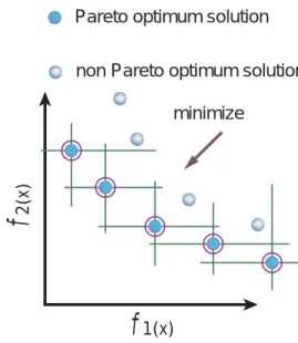
Usually, there is not only one Pareto optimum solution but plural solutions in MOPs. In Figure1, the concept of the Pareto optimum solutions are illustrated in the case of two objectives.
minimize
f 1(x)
2(x) f
Pareto optimum solution non Pareto optimum solution
Figure 1: The Pareto optimum solutions
In this figure, the line of the Pareto optimum solution is called a Pareto front. In MOPs, to find Pareto optimum solutions is one of the goals.
GENETIC ALGORITHMS FOR MOPS
The Genetic Algorithm is an algorithm that simulates crea- tures’ heredity and evolution[11]. Since the GA is one of the multi point search methods, an optimum solution can be determined even when the landscape of the objective function is multi modal. Moreover, the GA can be applied to problems whose search space is discrete. Therefore, the GA is one of very powerful optimization tools and is very easy to use. In multi-objective optimization, GA can find a Pareto optimum set with one trial because the GA is a multi point search. As a result, the GA is a very ef- fective tool especially in multi-objective optimization prob- lems. Thus, there are many researchers who are working on the multi-objective GA and there are many algorithms of the multi-objective GA[12, 13]. These algorithms of the multi-objective GA are roughly divided into two categories;
those are the algorithms that treat the Pareto optimum so-
lution implicitly or explicitly. The most of the latest meth-
ods treat the Pareto optimum solution explicitly. Typical
algorithms are SPEA2[14] and NSGA-II[15].
In the GAs, a searching point is called an individual.
Usually, an individual is express as a bit string. There are many ways to convert design variables to bit strings.
When the design variables are real numbers, the easiest way is to code the real number into the binary number.
The following steps are the basic procedure of the GAs for MOPs.
Step 1: It supposes there are m individuals. This means there are m search points. These individuals are initial- ized. Since each individual is shown as a bit string, each bit is determined using the random number.
Step 2: Each individual has fitness value. In this step, the fitness value of each individual is determined. This oper- ation is called ”Evaluation”. In MOPs, the Pareto ranking is often used for determining the fitness value[28]. The Pareto ranking is determined in the following procedure.
For each solution, the number of the solution that are dominant to the focused solution is counted. The Pareto ranking is this number + 1. When the solution is non- dominant, the Pareto ranking becomes 1. The concept of the Pareto ranking is shown in 2. In this figure R denotes the Pareto ranking. The fitness value of each individual is a reciprocal number of the Pareto ranking.
f
1f
2 Real Pareto Front R=1R=1
R=1 R=2 R=3
R=4
Figure 2: Pareto Ranking
Step 3: After the evaluation, with according to the fitness value, an individual is checked to remain for the next it- eration. This checking is performed probabilistically. The individual whose evaluation value is big has a high pos- sibility of remaining in the next iteration. There is a case where the individual who has high evaluation value may increase. On the other hand, the individual whose evalua- tion value is small may be disappeared. This operation is called ”Selection”. Usually, the roulette selection method is performed.
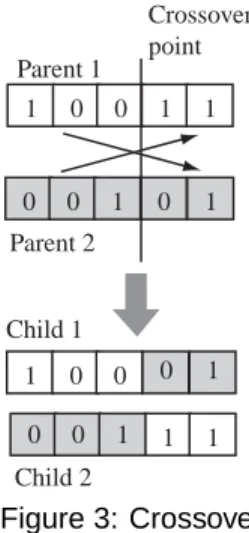
Step 4: New search point is created by operations of
”crossover” and ”mutation”. Two individuals are chosen randomly. Those are called parents. The crossover point is determined randomly. Then the first part of parent 1 and the latter part of parent 2 are combined. Again, the latter part of parent 1 and the first part of parent 2 are combined. These are children and those are new search points. This operation is called ”Crossover”. In Figure3,
the concept of crossover is shown.
1 0 0 1 1
0 1
0 0 1
Parent 1
Parent 2
Crossover point
1 0 0 0 1
1 1
0 0 1
Child 1
Child 2
Figure 3: Crossover
In the operation of mutation, a certain bit of individual is chosen randomly. When this bit is equal 1, it is changed into 0. This operation also generates a new search point.
In Figure4, the concept of mutation is shown.
1 0 0 1 1
0
1 0 0 1
Figure 4: Mutation
Step 5: If the terminal condition is not satisfied, the rou- tine is back to step 2. In GA, this one routine is often called
”Generation”. Usually, many generations are needed to find an optimum solution.
These steps are summarized in Figure5.
Initialization
Evaluation
Derive the Pareto ranking of each individual Pi.
Derive the fitness value of each individual Fi = 1/Pi.
Terminal
Check End
Crossover
Mutation yes
no k=1
k=k+1
Figure 5: Flow of GA
NEIGHBORHOOD CULTIVATION GENETIC ALGO- RITHM (NCGA)
OVERALL In this paper, an extended GA that is called
the Neighborhood Cultivation Genetic Algorithm (NCGA)
is used. The NCGA has the neighborhood crossover mechanism besides the mechanisms of SPEA2[14] and NSGA-II[15]. In the GAs, the exploration and exploita- tion are very important. By the exploration, an optimum solution can be found in a global area. By the exploita- tion, an optimum solution can be found around the elite solution. In the single object GA, the exploration is per- formed in the early stage of the search and the exploita- tion is performed in the latter stage. On the other hand, in the multi-objective GAs, both the exploration and ex- ploitation should be performed during the search. Usually, the crossover operation helps both the exploration and exploitation. In the NCGA, the exploitation factor of the crossover is reinforced. In the crossover operation of the NCGA, a pair of the individuals for crossover is not cho- sen randomly, but individuals who are close each other are chosen. Because of this operation, the child individu- als who are generated after the crossover may be close to the parent individuals. Therefore, the precise exploitation is expected.
THE FLOW OF NCGA The following steps are the over- all flow of the NCGA where
P
t: search population at generation t A
t: archive at generation t.
Step 1: Initialization: Generate an initial population P 0 . Population size is N . Set t = 0 . Calculate fitness values of initial individuals in P 0 . Copy P 0 into A 0 . Archive size is also N .
Step 2: Start new generation: Set t = t + 1.
Step 3: Generate new search population: P
t= A
t−1. Step 4: Sorting: Individuals of P
tare sorted with along to the values of focused objective. The focused objective is changed at every generation. For example, when there are three objectives, the first objective is focused in this step in the first generation. The third objective is focused in the third generation. Then the first objective is focused again in the fourth generation.
Step 5: Grouping: P
tis divided into groups which con- sist of two individuals. These two individuals are chosen from the top subsequently toward the bottom of the sorted individuals.
Step 6: Crossover and Mutation: In a group, the crossover and mutation operations are performed. From two parent individuals, two child individuals are gener- ated. Here, parent individuals are eliminated.
Step 7: Evaluation: All of the objectives of individuals are derived. According to the values of objectives, the Pareto ranking of each individual is decided. Using the Pareto ranking, the fitness value of each individual is decided.
This operation is the same as the step 2 in the former section.
Step 8: Assembling: The all individuals are assembled into one group and this becomes new P
t.
Step 9: Renewing archives: Assemble P
tand A
t−1to- gether. Then N individuals are chosen from 2 N individ- uals. To reduce the number of individuals, the same op- eration of the SPEA2 (Environment Selection) is also per- formed.
Step 10: Termination: Check the terminal condition. If it is satisfied, the simulation is terminated. If it is not satis- fied, the simulation returns to Step 2.
These steps are summarized as a schematic in Figure6.
In the NCGA, most of the genetic operations are per- formed in a group that is consisted of two individuals. That is why this algorithm is called ”Neighborhood cultivation”.
This scheme is similar to the Minimum Generation Gap model (MGG)[16]. However, the concept of generation of the NCGA is the same as the simple GAs.
NUMERICAL EXAMPLE To demonstrate the searching ability of the NCGA, the NCGA is applied to the typical test function, KUR. The results are compared with those of the SPEA2[14] and NSGA-II[15]. KUR was used by Kursawa [17].
KUR :
min f
1=
ni=1
(−10 exp(−0 . 2 x
2i+ x
2i+1)) min f
2=
ni=1
(| x
i|
0.8+ 5 sin( x
i)
3) s.t.
x
i[−5 , 5] , i = 1 , . . . , n, n = 100
(3)
It has a multi-modal function in one component and the pair-wise interactions among the variables in the other component. Since there are 100 design variables, it needs a high calculation cost to derive the solutions.
In the former studies, some methods used the real value coding and made good results[14]. In this paper, to dis- cuss the effectiveness of the algorithm, the simple meth- ods are applied for all the problems. Therefore, the bit coding is used in the experiments. Similarly, the one point crossover and bit flip are used for the crossover and mu- tation. The length of the chromosome is 20 bit per one design variable. Population size is 100 and the simulation is terminated when the generation is got over 250.
From Figures7 to 10, the derived Pareto solutions are
shown. Figure10is the result of the NCGA but without the
neighborhood crossover. In these figures, all the Pareto
optimum solutions that are derived in 30 trials are figured
At-1
Pt
At Copy
Sort
Crossover
Mutation
add
Selection
t=t+1
Figure 6: Flow of NCGA
out. There are several ways to compare the solutions[13].
One of them is to check the appearance of the derived solutions. Because this is the minimization problem, the solutions that are located in the left and bottom are bet- ter. At the same time, solutions should be spread instead of the concentration on one point. These two points can be ascertained by the appearance of the derived solu- tions. It is clear that the NCGA derived better solutions than the other methods. The solutions of the NCGA are also wider spread than those of the other methods. In this problem, the comparison between Figure7 and Figure10 shows that the mechanism of the neighborhood crossover acts effectively to derive the solutions. That is to say the neighborhood crossover is an operation to find the solu- tions that have the diversity and high accuracy.
–300 –250 –200 –150 –100 –50
–900 –800 –700
NCGA
f1(x)
f 2(x)
Figure 7: Results of KUR (NCGA)
–300 –250 –200 –150 –100 –50
–900 –800 –700
SPEA2
f1(x)
f 2(x)
Figure 8: Results of KUR (SPEA2)
300 –250 –200 –150 –100 –50
–900 –800 –700
–
NSGA-II
f1(x)
f 2(x)
Figure 9: Results of KUR (NSGA-II)
–300 –250 –200 –150 –100 –50
–900 –800 –700
nNCGA
f1(x)
f 2(x)
Figure 10: Results of KUR (NCGA without neighborhood crossover)
PHENOMENOLOGICAL MODEL AND HIDECS
In the work reported in this paper, the most sophis- ticated phenomenological spray-combustion model cur- rently available, originally developed at the University of Hiroshima had previously demonstrated potential as a predictive tool for both performance and emissions in sev- eral types of the direct injection diesel engine. Recently, we call the HIDECS to this model code. A detailed discus- sion of the HIDECS spray-combustion model and some examples of its previous applications are given in Refer- ence [18-25]. Therefore, only a brief description of the model is provided in this section.
The spray injected into the combustion chamber from the
injection nozzle is divided into many small packages of equal fuel mass as shown in Figure11. No intermixing among the packages is assumed. The spray charac- teristics are defined by the empirical equations of spray penetration. For example, the shaded regions shown in Figure11 are the fuel packages injected at the start of in- jection that constitute the spray tip during penetration. Air entrainment into a package is controlled by the conserva- tion of momentum, that is, the amount of entrained air is proportional to the decrease in package velocity. The fuel, which is mixed with the air, begins to evaporate as drops, and ignition occurs after some ignition-delay period.
Breakup Length Spray tip penetration Package pf Spray P(L, M, N)
M
L N
Injected at the start of injection
* No-intermixing among the package is assumed.
* Spray tip penetration is defined by the experimental equations
Figure 11: Schematic of the package distribution The air-fuel mixing processes within each package are il- lustrated in Figure12. Each package, immediately after the injection, involves many fine drops and a small amount of air. As a package moves away from the nozzle, air entrains into the package and the fuel drops evaporate.
Thus, the package consists of liquid drops, vaporized fuel, and air. After a short period of time following injection, ig- nition occurs in the gaseous mixture, resulting in the rapid expansion of the package. Therefore, more fuel drops Figure12. Schematic of the package combustion process evaporate, and more fresh air entrains into the package.
The vaporized fuel mixes with fresh air and combustion products as the spray continues to burn.
Air Entralnment Expansion & Air Entralnment
Injection Evaporation
& Mixing
Fuel Ignition &
Combustion
Evapolation Mixing &
Combustion
Mixing &
Combustion
Figure 12: Schematic of the mass system during combus- tion
Figure13 shows two possible combustion processes for each package. Case A is called evaporation- rate-controlled combustion, while Case B is called the entrainment-rate-controlled combustion. When ignition occurs, the combustion mixture that is prepared before ig- nition burns in a small increment of time. The fuel-burning rate in each package is calculated by assuming stoichio- metric combustion. When there is enough air in the pack- age to burn all of the vaporized fuel, there are combustion products, liquid fuel and fresh air remaining in the pack-
age after combustion (Case A in Figure13). In the next small increment of time, more fuel drops evaporate and fresher air entrains into the package. At this point, if the amount of air in the package is enough to burn all the vaporized fuel at the stoichiometric condition, the same combustion process (Case A) is repeated. If the amount of air is not enough to burn all the vaporized fuel, how- ever, the fuel-burning rate is dictated by the amount of air present (Case B in Figure13). Therefore, the combustion processes in each package always proceed under one of the conditions shown in Figure13.
The heat release rate in the combustion chamber is calcu- lated by summing the heat release of each package. The cylinder pressure and bulk-gas temperature in the cylin- der are then calculated. Since the time history of temper- ature, vaporized fuel, air and combustion products in each package are known, the equilibrium concentrations of gas composition in each package can be calculated. The con- centration of NOx is calculated by using the extended Zel- dovich mechanism. The formation of soot is calculated by assuming first-order reaction of fuel vapor. The oxidation of carbon is calculated by assuming second-order reac- tion between carbon and oxygen.
: Liquid Fuel : Vaporized Fuel : Air
: Products
(A) (B)
Controlled by Air Entrainment Rate Controlled by Air Fuel
Evaporation Rate
(A) (B)
Injection
Ignition Combustion
Valve Open
Complete Combustion Incomplete Combustion
Figure 13: Schematic of the package combustion process
HIDECS/NCGA SIMULATION EXAMPLE
OVERALL The HIDECS can deal with several types of diesel engines. In this simulation, the specification of the target diesel engine is summarized in Table1.
In this engine used in a simulation, the fuel injection starts at -5.0 ATDC degree and the injection is lasted for 18 degrees. The total amount of fuel injection is constant, but the shape of the fuel injection can be changed. This shape of the fuel injection is a design variable in this sim- ulation.
The HIDECS can derive several characteristics of en-
gines. In this simulation, SFC, the amount of NOx and
the amount of Soot are focused.
Table 1: Specification of the target diesel engine
Bore 102 mm
Stroke 105 mm
Compression Ratio 17
Engine Speed 1800 rpm
Swirl Ratio 1.0
Nozzle Hole Diameter 0.2 mm
Nozzle Hole Number 4
hline Injected Fuel Volume 40.0 mg/st Injection Timing -5.0 ATDC deg.
Injection Duration 18 deg.
SYSTEM CONSTRUCTION The overview of the sys- tem is written in Figure14.
NCGA wrapper
HIDECS
input file
output file
optimizer analyzer
Figure 14: System construction
In Figure14, the NCGA is used as an optimizer and the HIDECS is used as an analyzer. Between the optimizer and analyzer, text files are exchanged. Therefore, basi- cally several types of the GAs and analyzers can be used in this system.
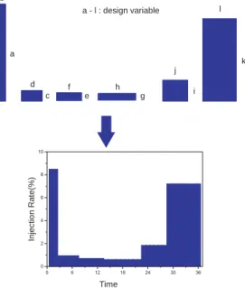
In this simulation, the amount of SFC, the amount of NOx and the amount of Soot are the objectives. The split in- jection rate-shape is a design variable. In this simulation, the total amount of fuel injection, the start of the injection and the duration of the injection are fixed. On the other hand, the injection rate is a variable. The shape of the in- jection rate can be defined as follows. The duration of the injection is divided into 6 blocks. Each block has its own width and height. When these widths and heights are de- termined, the shape of the injection rate is determined.
Therefore, the NCGA decides these values.
In Figure15, the concept of coding method is summarized.
There are 12 variables (6 blocks have their widths and heights). These are real values which are from 0.0 to 1.0.
They are coded into 8 bits by gray coding. Because the amount of the fuel and the duration of injection are fixed, the total area of 6 blocks is also fixed.
GA PARAMETERS In this simulation, the following pa- rameters are used. The length of the chromosome is 8 bit per one design variable. Therefore, the total length of the chromosome is 96. The population size is 100 and the
a b
c d
e f
g
h i
j
k a - l : design variable l
Time
Injection Rate(%)
Figure 15: Coding method
number of sub population is 10. The crossover rate and mutation rate are 1.0 and 1/96 respectively. At the same time, migration rate and migration interval are 0.4 and 10 respectively. We use two point crossover and tournament selection. The simulation is terminated when the genera- tion is over 200.
RESULTS In this section, the derived Pareto optimum solutions are described. The characteristics of the de- rived shape of injection rate are discussed briefly. The most important aspect of the multi-objective optimization problems is that the designers can find their design alter- natives. The design alternatives are discussed using the derived Pareto solutions. The end of this section, the topic of calculation cost is mentioned.
Pareto-optimum solutions In Figure16, the derived Pareto solutions are plotted. In the figure, all the plotted solutions dominant to the other solutions that are derived during search. In Figures17, 18 and 19, the derived so- lutions are projected on SFC-NOx, SFC-Soot and NOx- Soot surface respectively.
From these figures, it is found that the Pareto solutions are derived.
In Figures20, 21 and 22, the solutions who have the best value of each objective function are illustrated.
In the solution who has the smallest value of SFC, the
fuel injection pattern is characterized with the most fuel
injected at the beginning of injection duration. In the solu-
tion who has the smallest value of NOx, the fuel is injected
at two steps. In the solution who has the smallest value
of smoke, the fuel is mostly injected in the middle of the
injection period.
200 240
280 0.2
0.4 0.8
1.2 1.6
NOx (g/kWh)
SMOKE (g/kwh)
SFC (g/kwh)
Figure 16: Derived Pareto solutions (SFC, NOx, Smoke))
180 200 220 240 260 280 300
0.4 0.6 0.8 1.0 1.2 1.4 1.6 1.8
NOx (g/kWh)
SFC (g/kWh)
Figure 17: Derived Pareto solutions (SFC, NOx)
The early fuel injection gives the best solution of SFC (shown in Figure20). The early injection causes better fuel-air-mixing at the early stage of the combustion pro- cess, which results high maximum in-cylinder pressure and high engine output. In the pattern shown in Figure21, some of the fuel is injected at the beginning of injection and the rest of them at the end of injection. This dou- ble step injection, known as pilot injection, can reduce the NOx emission, because the medium in-cylinder pressure can be obtained to prevent the NOx formation. The op- timum solution is in the agreement with the experimental studies on the pilot injection. It is very interesting to find out that the smallest smoke emission is obtained by inject- ing the most fuel at the middle of the injection period. This may be caused by the reduction of the incomplete fuel combustion in the combustion stroke. The small amount of fuel injected in the early stage evaporates and com- busts. This operation may help the rest of fuel combust completely in a better environment.
From Figures16 to 22, it can also be found that there ex- ists a conflict between economy and emissions control.
There has to be a compromised fuel injection pattern to obtain the low emissions according to the increasing strict
180 200 220 240 260 280 300
0.08 0.10 0.12 0.14 0.16 0.18 0.20 0.22 0.24 0.26 0.28
SMOKE (g/kWh)
SFC (g/kWh)
Figure 18: Derived Pareto solutions (SFC, Smoke)
0.4 0.6 0.8 1.0 1.2 1.4 1.6 1.8
0.08 0.10 0.12 0.14 0.16 0.18 0.20 0.22 0.24 0.26 0.28
SMOKE (g/kWh)
NOx (g/kWh)
Figure 19: Derived Pareto solutions (NOx, Smoke)
regulations while keeping an acceptable SFC. It will be very costly to find such an injection pattern experimen- tally. Therefore, computation methods show the most ad- vantage in model engine design. In the following session, more will be discussed how to use the HIDECS as a de- sign tool with the aid of the NCGA.
Design alternative In Figure23, the Pareto optimum so- lutions are projected on the NOx and SFC surface. It is the same as Figure17. In this figure, we select the four design alternatives and they are plotted.
The selection method of design alternatives from the de- rived Pareto solutions is a hot topic in MOPs[13]. In this paper, the design alternatives are chosen in the following way. The candidate number one is the solution that has the best value of SFC. The candidate number two is the closest solution to the number one. The candidate num- ber four is also the solution that has the best value of NOx.
The candidate number three is the divergence solution.
Figure23 can be simplified and it is shown in Figure24.
The change ratio of NOx with along to SFC is changed at the candidate 3. Therefore, the solutions can be classified into two groups those are shown in Figure24 as A and B.
In A group, the change ratio is relatively big. Therefore,
5 10 15 20 25 30 35 0
5 10 15 20 25 30
Injection Rate (%)
Injection Timing
Figure 20: Pareto optimum solution that has the smallest value of SFC (SFC=183.7, NOx=1.743, Smoke=0.2605) (Design candidate number 1 in Figure 20
5 10 15 20 25 30 35
0 2 4 6 8 10
Injection Rate (%)
Injection Timing
Figure 21: Pareto optimum solution that has the smallest value of NOx (SFC=299.6, NOx=0.4309, Smoke=0.1539) (Design candidate number 4 in Figure 20
even when NOx and SFC of two solutions are similar, the shape of the injection ratio of these solutions may be to- tally different. On the other hand, in B group, the change ratio is relatively small. Therefore, when the NOx and SFC of two solutions are totally different, the shape of the in- jection ratio of these solutions may be similar.
The candidate number 1 is the same as the solution shown in Figure20 and the candidate number 4 is the same as the solution shown in Figure21. The injection rate shapes of the candidates of number 2 and number 3 are shown in Figures25 and 26.
When the designer needs the good SFC, he chooses the candidate number 1. On the other hand, the designer needs the good NOx, he chooses the candidate number 4. The candidate number 1 and 4 are the same results when the one objective is minimized. However, the most important fact is that these results are derived by one trial.
At the same time, the designer can distinguish the solution distribution.
5 10 15 20 25 30 35
0 2 4 6 8 10
Injection Rate (%)
Injection Timing
Figure 22: Pareto optimum solution that has the smallest value of Smoke (SFC=267.8, NOx=1.050, Smoke=0.09924)
180 200 220 240 260 280 300
0.4 0.6 0.8 1.0 1.2 1.4 1.6 1.8
NOx (g/kWh)
SFC (g/kWh)
1 2
3
4
Figure 23: Pareto optimum solutions and design candi- dates
Compared to the candidate number 3 and 4, there are no big differences between them. Therefore, in this case, the candidate number 3 is the reasonable choice for the designer.
The following situation may be assumed. At first, the de- signer needs the result that has the lowest SFC. After, he gets this result, he may change his mind because he can find the candidate number 2 that has almost the same value for SFC but the value of NOx is much smaller.
From these results, the following advantages of the GAs for multi-objective optimization problems are confirmed.
• the GAs can find the Pareto optimum solutions with
one trial. In a single objective optimization problem,
the GAs need the high calculation cost compared to
the gradient search methods. On the other hand, in
a multi-objective optimization problem, the gradient
search methods also need many iterations to find the
Pareto optimum solutions. The GAs are very easy to
apply several types of problems. At the same time,
the GAs have the robustness in finding the optimum
NOx
SFC 1
3
4
A
B
Figure 24: Design candidates
Injection Rate (%)
Injection Timing
0 2 4 6 8 10
5 10 15 20 25 30 35
Figure 25: Design candidate number 2 (SFC=184.4, NOx=1.5149, Smoke=0.2585)
solution in a global area. Thus, the GAs are very useful tools to find Pareto optimum solution.
• Usually, a multi-objective problem is turned into a sin- gle objective problem by setting an evaluation func- tion when the solutions are derived by the gradient search method. However, it is very difficult to set up this evaluation function. This evaluation function af- fects the results. On the other hand, GAs can find the Pareto optimum solutions without setting this excess evaluation function.
• In the results of this paper, the solutions that mini- mize each objective are totally different since there are the trade-off relations between the objective func- tions. Especially in the early stage of design, de- signers do not know the relationship between the ob- jectives. Therefore, it is very useful for designers to show the Pareto optimum solutions. The designers can find solutions with their preferences.
• Even when the problems are in the bottom stage of design and the designers know the relationship be- tween the objective functions, it is useful to derive the solutions by the GAs. To solve the problem, the de- signers have to define the objective function and the constraints. At the same time, they define the val- ues of the constraints. Usually, the solutions are on the constraints. Therefore, the designers should be
5 10 15 20 25 30 35
0 2 4 6 8 10