Numerical and Experimental Studies on Dynamic Load Testing of Open-ended Pipe Piles and its Applications

(1)

Numerical and Experimental Studies on Dynamic Load Testing of Open‑ended Pipe Piles and its Applications

著者ファンタレ

著者別表示 Phan Ta Le journal or

publication title

博士論文本文full 学位授与番号 13301甲第3962号

学位名博士(工学)

学位授与年月日 2013‑09‑26

URL http://hdl.handle.net/2297/39365

Creative Commons : 表示 ‑ 非営利 ‑ 改変禁止 http://creativecommons.org/licenses/by‑nc‑nd/3.0/deed.ja

(2)

i

Numerical and Experimental Studies on

Dynamic Load Testing of Open-ended Pipe Piles and its Applications

開端杭の動的載荷試験に関する解析的・実験的研究とその適用

Phan Ta Le

Sep, 2013

(3)

ii

Dissertation

Numerical and Experimental Studies on

Dynamic Load Testing of Open-ended Pipe Piles and its Applications

開端杭の動的載荷試験に関する解析的・実験的研究とその適用

Graduate School of

Natural Science and Technology Kanazawa University

Division of Environmental Science and Engineering Course: Environment Creation

School registration No.: 1023142420

Name: Phan Ta Le

Chief advisor: Matsumoto Tatsunori

(4)

i

Abstract

Open-ended pipe piles are widely used in practice for foundations of various structures in both on-land and offshore foundations. They transfer loads from a superstructure to a medium or dense stratum through soft soil layers. When driving an open-ended pipe pile into soils, a part of soils around a pile toe intrudes into inside the pile to form a soil column called soil plug. Theoretically, bearing capacity of an open- ended pipe pile can be calculated from outer shaft resistance, toe resistance and soil plug resistance. In practice, the bearing capacity of a pile can be determined from static load test (SLT) or dynamic load test (DLT). Static load tests are regarded as reliable methods but they are costly and time-consuming, compared to dynamic load tests. Due to the high cost and long test period, SLTs are preserved for large-budget and important projects, and the number of the test piles are usually limited to 1 to 2 % of the working piles. Meanwhile dynamic load tests are quick, low cost and very effective in offshore conditions. With the similar budget for testing, we can carry out up to 10% to 20% number of the working piles. Such larger number of test piles results in the high reliability of the whole foundation solution to the construction site in which soil conditions are varied from distance to distance, compared to the case with only a few static load tests.

Additionally, the accurate prediction of the driving response is a key factor to select a suitable hammer system that minimise the damage of the pile during driving.

Also, it can help us to find out a suitable pile length with satisfying the requirements of both bearing capacity and settlement. In the dynamic load testing, wave matching analysis (WMA) plays a key role to identify soil properties and then to derive the static load-displacement relation. Conventionally, Smith’s method, characteristic solutions of the wave equation and a finite differential scheme have been used for wave matching analysis of the one-dimensional stress wave propagation in a pile.

However, when soil stiffness and velocity-dependent resistance have large values, these methods tend to show numerical instability. One of the reasons is that pile responses at current step in these methods are calculated based on the soil resistance mobilised at the previous calculation step. In other words, the pile behaviour and soil resistance are not fully coupled at a time step. More rigorous methods in which soils surrounding pile are regarded as a continuum media using finite element method, or

(5)

ii

finite difference methods have been developed, but they are too computational expensive with computational time of several hours or days, resulting in the difficulty in using continuum methods in routine pile dynamic analysis in practice.

Therefore, a matrix form calculation procedure of the one-dimensional stress wave theory is proposed in this thesis to improve the above mentioned shortcomings.

In the proposed numerical method, rational soil resistance models introduced by Randolph and Deeks (1992) are implemented. Effect of the wave propagation in the soil plug is modelled and taken into account. Furthermore, nonlinearity of soil stiffness and radiation damping in the soil models are considered. The proposed method can also be used for the analysis of static loading of the pile, if damping and inertia of the pile and the soil are neglected.

In order to verify the proposed numerical method, firstly, an open-ended pipe pile with soil resistance was analysed, and compared with results obtained from the Smith method and the rigorous continuum method, FLAC^3D. The analysed results showed that the proposed method has higher accuracy compared to the Smith method and shorter calculation time compared to the rigorous continuum method FLAC^3D. Secondly, verification of the proposed method was conducted by analysing the experimental results obtained from two series of static and dynamic load tests of an open-ended pipe pile and a close-ended pipe pile in model ground of dry sand. The proposed method predicted the static response of both piles with reasonable accuracy.

Plugging mode of the open-ended pipe pile under static and dynamic loading conditions can also be simulated using the proposed method. Thirdly, the proposed method was used to analyses the static load tests (SLTs) and dynamic load tests (DLTs) of two open-ended steel pipe piles and two spun concrete piles in a construction site in Viet Nam. The analysed results showed that the static load-displacement curves derived from the final WMAs of DLTs were comparable with the results obtained from the SLTs. WMA using the proposed numerical approach well predicted the static load-displacement curves of the non-tested working piles based on the identified soil parameters of the tested piles. Also, from calculated analyses using the proposed method, the piles which have been subjected to cyclic loading had smaller yield and ultimate capacities compared to the piles subjected to monotonic loading. Finally, the proposed method reasonably estimated static cone resistance of the dynamic cone penetration tests with dynamic measurements.

(6)

iii

Acknowledgments

This thesis would not have been possible without the great support and cooperation of many individuals during 3 years of study and research in Geotechnical Laboratory of the Kanazawa University. It is an honour for me to express my sincere words here.

First of all, it would like to express my deepest gratitude to my supervisor, Pro- fessor Tatsunori Matsumoto, for his sincere support, valuable discussions and experienced guidance on my study. This thesis would not have been possible without his dedicated help. Under his enthusiastic supervision, I have learnt a lot of things from how to prepare and write a technical paper as well as a thesis to how to present effectively in an international conference. I was also very impressed and admired by his profound knowledge and great interest in doing research.

I wish to express my sincere thankfulness to Associate Professor Shun-ichi Ko- bayashi for his kind guidance, valuable comments and various informative ideas on my research.

I also would like to show my gratitude to Prof. Hiroshi Masuya, Prof. Masa- katsu Miyajima and Prof. Shinichi Igarashi for their valuable comments on my thesis and their serving as members of my doctoral examination committee.

Special appreciations are going to Mr Shinya Shimono, technician of the Ge- otechnical Laboratory, and other students for many supports in my experimental work and my living. I highly appreciate to all the dedicated supports from staff of Kanaza- wa University.

I am also indebted to the scholarship sponsor, Vietnamese government, who supports all of the expense for my living and studying for 3 years in Japan.

Lastly, from my heart, I would like to express my cordially thanks to my be- loved wife, who takes care of my children instead of me and continuously encourage me during my study in Japan. I also highly appreciate to my parents, my brothers and my sisters for all their supports and encouragements at all time.

PHAN TA LE

(7)

iv

List of Figures

Figure 2.1. Standard, RSP and Maximum, RMX, Case Method Capacity Estimates ... 11

Figure 2.2. Numerical modelling and notation used in characteristic solution ... 13

Figure 2.3. Numerical modelling in Smith’s method ... 15

Figure 2.4. Notation used in finite difference scheme. ... 17

Figure 2.5. Energy transmission and absorption, and deformation mechanism in the soil around the pile shaft and at the pile base during pile driving. ... 18

Figure 2.6. Smith’s resistance soil models: (a) for pile shaft and (b) for pile base. ... 20

Figure 2.7. Shaft soil resistance model by Holeyman (1985)... 22

Figure 2.8. Shaft soil resistance model according to Randolph and Simons (1986). ... 23

Figure 2.9. Lysmer’s base soil resistance model. ... 25

Figure 2.10. Base soil resistance model developed by Deeks and Randolph (1992). ... 26

Figure 3.1. Pile – soil system. ... 33

Figure 3.2. Shaft soil model. Figure 3.3. Base soil model. ... 34

Figure 3.4. Non-linear soil response. ... 37

Figure 3.5. Head force and specification of the pile. ... 40

Figure 3.6. Comparison of the pile response at the middle point of the pile between the proposed method and the theoretical solution. (a) Pile axial force. (b) Pile velocity. ... 40

Figure 3.7. Specifications of the pile and soil. ... 41

Figure 3.8. Impact force with different loading durations. ... 41

Figure 3.9. Pile head displacements vs. time. ... 42

Figure 3.10. Modelling of the pile and ground using FLAC^3D. ... 43

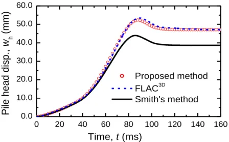
Figure 3.11. Pile head displacements of the open-ended pile obtained from the three methods. ... 44

Figure 4.1. Test results of DSTs and its approximations with c’=0 ... 51

Figure 4.2. Arrangement of the strain gauge. ... 52

Figure 4.3. Photo of the static load test system. ... 53

Figure 4.4. Photo of the pile driving system. ... 54

Figure 4.5. Load-displacement curves of the CP. ... 55

Figure 4.6. Mobilised soil resistance vs. local pile disp. of the CP in SLT2 at. ... 55

Figure 4.7. Comparison of the axial forces between the compression and tension tests. ... 56

Figure 4.8. Relationship between the confined modulus, Ec, with overburden stress,_v^'.. 58

(11)

viii

Figure 4.9. Soil properties used in the first WMA of the CP. ... 59

Figure 4.10. Measured axial force at SG1 of blow 5 of the CP. ... 59

Figure 4.11. Results of the final WMA of the CP for the axial forces. ... 60

Figure 4.12. Pile head displacement calculated from the final WMA of the CP. ... 61

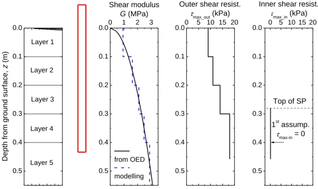
Figure 4.13. Distribution of the shear moduli and shear resistances. ... 61

Figure 4.14. Derived and measured static load-displacement curves of the CP... 62

Figure 4.15. Derived and measured distributions of the axial forces of the CP. ... 63

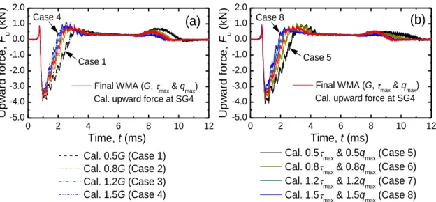
Figure 4.16. Sensitivity of the axial force at SG4 due to. ... 65

Figure 4.17. Sensitivity of the upward force at SG4 due to. ... 66

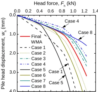
Figure 4.18. Sensitivity of the pile head disp. due to ... 66

Figure 4.19. Variation of the static load-displacement curves of the CP. ... 67

Figure 4.20. Location of the pile and change of the soil plug height at the end of each stage. ... 68

Figure 4.21. Load-displacement curves of the OP. ... 69

Figure 4.22. Relationship between the shear resistance, , and the local pile displacement, w, of the OP in SLT2. ... 69

Figure 4.23. Soil properties used in the first WMA of the OP. ... 70

Figure 4.24. Measured axial force at SG1 of blow 10 of the OP. ... 71

Figure 4.25. Results of the final WMA of the OP for the axial forces. ... 71

Figure 4.26. Displacements of the pile head and the top of soil plug calculated in the final WMA of the OP. ... 72

Figure 4.27. Distribution of the shear moduli and shear resistances. (a) Outer shear moduli. (b) Outer shear resistances. (c) Inner shear moduli. (d) Inner shear resistances. ... 73

Figure 4.28. Derived and measured static load-displacement curves of the OP. ... 74

Figure 4.29. Derived and measured distributions of the axial forces of the OP. ... 74

Figure 4.30. Derived and measured static load-displacement curves of the OP and CP. ... 75

Figure 5.1. Location of the site. ... 78

Figure 5.2. Photo of the berth area prior to in use. ... 78

Figure 5.3. Locations of the boreholes, test piles and working piles... 80

Figure 5.4. Geological sections at locations of the test piles. (a) TSP1. (b) TSC1. ... 81

Figure 5.5. Geological sections at locations of the test piles. ... 82

Figure 5.6. Estimated shear modulus at the four test piles. ... 83

Figure 5.7. Estimated ultimate capacity with depth and selection of the pile tip level. ... 86

(12)

ix

Figure 5.8. Pile combination from its segments. ... 88

Figure 5.9. Illustration of the four test pileS before and after cutting the pile to the cut-off level. (a) TSC1. (b) TSC2. (c) TSP1. (d) TSP2. ... 90

Figure 5.10. Illustration of the test pile driving by diesel hammer... 91

Figure 5.11. Illustration of the SLT. (a) Layout of the test piles and reaction system. ... 93

Figure 5.12. Uplift capacity of the anchor piles with the soil conditions at the TSC1, TSC2, TSP1 and TSP2. ... 94

Figure 5.13. Loading process in SLTs. ... 95

Figure 5.14. Modelling of the test ground at the test pile TSC1. ... 97

Figure 5.15. Modelling of the test ground at the test pile TSP1. ... 97

Figure 5.16. Calculated impact forces at the pile head, together with measured forces .... 98

Figure 5.17. Calculated impact forces at the pile head, together with measured forces .... 98

Figure 5.18. Results of the final wave matching analysis of EOD test of the TSC1. ... 100

Figure 5.19. Results of the final wave matching analysis of BOR test of the TSC1 ... 100

Figure 5.20. Soil properties obtained from the final WMA of the TSC1 ... 101

Figure 5.21. Calculated pile head displacement with different heights of the soil plug. . 103

Figure 5.22. Distribution with depth of the maximum tensile and compressive stresses in the pile during driving of the TSC1. ... 103

Figure 5.23. Comparison of the static load displacement curves of the TSC1. ... 104

Figure 5.24. Calculated distributions with depth of the pile axial forces of the TSC1 .... 105

Figure 5.25. Calculated distributions with depth of the pile axial forces of the TSC1 at the BOR test for three loading processes. ... 106

Figure 5.26. Results of the final wave matching analysis of EOD test of the TSP1. ... 108

Figure 5.27. Results of the final wave matching analysis of BOR test of the TSP1 ... 108

Figure 5.28. Soil properties obtained from the final WMA of the TSP1 ... 108

Figure 5.29. Distributions with depth of the maximum tensile and compressive stresses in the pile during driving of the TSP1. ... 109

Figure 5.30. Comparison of static load displacement curves of the TSP1. ... 110

Figure 5.31. Distribution with depth of pile axial forces at different applied load of the TSP1. ... 111

Figure 5.32. Calculated distributions with depth of the pile axial forces of the TSC1 at BOR test at the working load for three loading processes. ... 112

Figure 5.33. Calculated load-displacement curves with and without cyclic loading, together with the result of SLT of the TSP1. ... 113

(13)

x

Figure 5.34. Comparison of the static load displacement curves of the TSC2. ... 114

Figure 5.35. Comparison of the static load displacement curves of the TSP2. ... 115

Figure 6.1.Various types of DCPT devices ... 121

Figure 6.2.Various types of driving rods of DCPTs and SPT instrumented with strain gauges ... 122

Figure 6.3. Results of measured driving energy of a blow in a DCPT with dynamic meaurement ... 124

Figure 6.4. Results of measured driving energy of a blow in SPT with dynamic meaurement ... 124

Figure 6.5. Results of DCPTs and SPT with dynamic measurement. ... 126

Figure 6.6. Illustration of a DCPT with dynamic measurement. ... 127

Figure 6.7. Modelling of the driving rod in WMA. ... 128

Figure 6.8. Modelling of the driving rod and soil... 129

Figure 6.9. Measured dynamic signals of Blow 12.1 using hammer mass of 3 kg. ... 130

Figure 6.10. Measured dynamic signals of Blow 12.2 using hammer mass of 5 kg. ... 130

Figure 6.11. Results of the final WMA of Blow 12.1. (a) Downward traveling force. (b) Displacement at SG level. ... 131

Figure 6.12. Results of the final WMA of Blow 12.2 (a) Downward traveling force. (b) Displacement at SG level. ... 131

Figure 6.13. Results of the final WMA of Blow 12.2 (a) Outer shear moduli. (b) Outer shear resistances. ... 132

Figure 6.14. Comparison of static cone resistance from CPT and from WMA ... 132

(14)

xi

List of Tables

Table 2.1. CASE damping factors for estimation of static capacity ... 11

Table 4.1. Physical properties of the Silica sand. ... 51

Table 4.2. Internal friction angle of the Silica sand. ... 51

Table 4.3. Properties of the model pile. ... 52

Table 4.4. Driving conditions and measured set per blow of DLTs of the CP. ... 57

Table 4.5. Driving conditions and measured set per blow of DLTs of the OP. ... 70

Table 5.1. Working load and corresponding allowable set. Table 5.2. Required capacity. ... 84

Table 5.3. Specification of test piles. ... 86

Table 5.4. Required energy for pile driving hammer and condition for hammer mass. ... 87

Table 5.5. Specification of the pile driving hammer. ... 88

Table 5.6. The maximum settlement per blow of the four test piles. ... 89

Table 5.7. Schedule for the test piles. ... 90

Table 5.8. The maximum test load. ... 92

Table 5.9. Elastic shortening of the pile and the allowable pile head displacements. ... 96

Table 5.10. The soil parameters at the pile tip and soil plug base obtained ... 101

Table 5.11. Soil parameters at the pile tip and soil plug base obtained from the final WMA. ... 109

Table 6.1. Specifications of driving rods of various DCPTs and SPT. ... 120

Table 6.2. DCPT and SPT with various hammers, anvils, rods, cones and impact energies. ... 120

Table 6.3. Summary of driving efficiency of various types of DCPTs and SPT. ... 125

(15)

1

Chapter 1 Introduction

In this introduction chapter, the background and motivation of the thesis is explained firstly.

Then, the objective of the thesis is presented. Finally, the organization of the thesis is given in the last section of the chapter.

1.1 Background and motivation

Pile foundations are predominantly employed to transfer large superstructure loads to the ground at sites where shallow foundations cannot be used due to the existence of soft clay or loose sand layers. They may be required to carry uplift loads when used to support tall structures subjected to overturning forces from winds. Piles used in offshore conditions are usually subjected to lateral loads from the impact of berthing ships and from waves. Combi- nations of vertical and horizontal loads are carried where piles are used to support retaining walls, bridge piers and abutments, and machinery foundations. In terms of subjecting to compressive axial load, the capacity of the pile is the sum of two components, namely shaft friction and base resistance. In case of an open-ended pipe pile, the capacity of the pile consists of three components: outer shaft resistance, pile tip resistance and soil plug base resistance. A pile in which the shaft-frictional component predominates is known as a friction pile, while a pile bearing on rock or some other hard incompressible ground is known as an end-bearing pile.

The mobilisation of limit shaft resistance requires small pile head displacements (about 0.2 to 0.5 % of the pile diameter), whereas much larger head displacements (about 2 to 4 %, even up to 5 to 10 % of the pile diameter in case of nonlinear soil response) are required for full mobilisation of base resistance. Depending on the installation method, most piles are

(16)

2

categorised into two main types: non-displacement piles or displacement piles. Non- displacement piles are cast-in-place piles installed by first removing the soil by a drilling process and then constructing the pile by pouring concrete or grout in the created void space.

This installation process causes only small disturbance to the surrounding soil, nearly remain- ing the initial stress state and soil density. Meanwhile, displacement piles are inserted into the ground by driving or jacking without prior removal of the soil from the ground. This process make the soil reduce the void ratio and generate the high excess pore-water pressure, resulting in the remarkable change of the initial stress state and soil density. Generally, displacement piles have larger capacity than non-displacement piles with the same pile configurations.

Regardless of pile types, the methods used for the determination of pile capacity prior to their installations are categorised into two main methods:

1) Methods based on soil properties determined from laboratory tests.

2) Methods based on in situ tests such as SPT, CPT or DCPT

These design methods are regarded as the so-called static methods. Although pile foundations are very common today and usually employed for supporting heavy and important structures, the most popular and well established methods for the determination of the shaft and base resistances in practice still contain a significant degree of uncertainty and base on the empirical equations, which limits their effectiveness and the wideness of their applicability.

As a consequence, foundation engineers often rely on dynamic or static pile testing for verifying the pile capacity and re-evaluating the foundation design prior to construction.

At present, the most common pile load test methods are static load tests (SLTs) and dynamic pile load tests (DLTs). Although SLTs are simple in concept, they are costly, time- consuming and usually used for large-budget and important projects. In DLT, pile acceleration and axial strain at the pile head are recorded during driving in a very short period, about 0.1 s. Then, pile head velocity and displacement histories are calculated from the measured acceleration history through numerical integration technique. Meanwhile, the measured strain is used for calculating the axial force history at the pile head. Wave matching analysis is conducted to identify the soil parameters and then to derive the static load-displacement relation. As far as known, determination of the pile capacity from static pile tests is simple, direct and straightforward. However, only about 1 to 2 % of working piles are selected for the SLT, resulting in a low reliability of the whole foundation solution to the construction sites in which soil condition varies from distance to distance. In these situations, number of the test piles has to increase in order to ensure the reliability of the whole foundation solution. In this aspect, DLT is a promising testing method due to its low cost and short test period. With the

(17)

3

similar budget for testing, number of DLTs test can increase up to 10 to 20% of the working piles, resulting in a high reliability of the whole foundation solution. In other words, we can reduce factor of safety or cut down the cost of the project without reduction of safety of the foundation solution. Therefore, research on dynamic analysis of DLTs is essential to seek for an efficient foundation solution to the structure. Although DLT is quick and efficient compared to SLT, pile capacity estimated from dynamic load tests has always been more challenging and require sophisticated dynamic analysis.

Early efforts in pile dynamics with consideration of the propagation of the one- dimensional stress wave in a pile was made by Smith (1960). In this approach, the pile was modelled as a series of lumped masses interconnected by massless linear springs and the problem was solved using numerical integration technique. In the following decades, several improvements were made to the original work by Smith (e.g. Goble and Rausche 1976, Simons and Randolph 1985, Lee et al. 1988, Rausche et al. 1994, Hussein et al. 1995).

Alternative techniques were also proposed for analysing pile driving, such as finite element analysis (e.g. Borja 1988, Nath 1990, Deeks 1992, Mabsout et al. 1995, Liyanapathirana et al.

2000, Masouleh and Fakharian 2007), closed-form solutions (e.g. Hansen and Denver 1980, Uto et al. 1985, Wang 1988, Warrington 1997), characteristic solutions (e.g. De Josselin De Jong 1956, Coyle and Gibson 1970, Heerema 1979, Van Koten et al. 1980, Middendorp and van Weele 1986, Matsumoto and Takei 1991, Courage and van Foeken 1992, Foeken et al.

1996) or finite difference scheme (Wakisaka and Matsumoto 2004).

At present, there are some computer programs using different methods developed for pile driving analysis based on the one-dimensional stress-wave propagation in a single pile.

For example, CAPWAP (Goble et al 1976, Rausche et al. 1985) uses Smith method, TNOWAVE (Middendorp et al. 1986), KWAVE (Matsumoto et al. 1991) use characteristic solution, KWAVEFD (Wakasaki et al. 2004) uses finite difference scheme. However, they have still limitations because the pile behaviours and soil resistances in these methods are not fully coupled at a time step. Paik et al. (2003) found that although a good matching is obtained from WMA using CAPWAP program, it still underestimates significantly the load capacity of both closed- and open-ended piles for the conditions investigated by these authors.

Beside of limitations of the current WMA due to the numerical method, this might also cause by the soil resistance models or numerical modelling of pile-soil system. Hence, it is needed to improve in the numerical approach with appropriate numerical modelling and realistic soil resistance models to enhance the reliability of the current dynamic analysis.

(18)

4

1.2 Objective

The main objectives of this research are provided as follows:

1. Improve the limitations in the current pile dynamic analysis by proposing a numerical method using a matrix form to analyse the phenomenon of wave propagation in an open-ended pipe pile within a framework of one-dimensional stress-wave theory.

2. Reveal the reliability and higher accuracy of the proposed method compared to the conventional methods through verification work which starts from numerical analysis to analyses of small-scale model tests and full-scale tests.

3. Demonstrate the advantage of dynamic cone penetration tests (DCPTs) with dynamic measurements as well as use the proposed numerical method for identifying the soil resistance acting on the driving rod and cone tip of DCPTs.

1.3 Thesis structure

The thesis consists of the following chapters

Chapter 1 is the introduction chapter of this thesis.

Chapter 2 deals with related research works. Section 2.1 briefly summarised the cur- rent pile dynamic analysis methods. Then, mechanisms of soil resistance mobilised along pile shaft and at the pile tip were presented. After that, soil resistance models used in pile driving analysis were reviewed and discussed.

Chapter 3 presents a numerical method based on the one-dimensional stress-wave theo- ry using the rational soil models with some modifications proposed by the authors such as non-linearity of soil stiffness and radiation damping. In order to validate the proposed numerical method, some numerical analyses were conducted by comparison the calculated results with those obtained from the theoretical solution, Smith’s method and FLAC^3D calculation.

In Chapter 4, further validation was conducted using a small scale model in laboratory.

First, element tests were carried out to determine initial soil parameters that would be used in dynamic analysis. Second, two series of pile load tests of open-ended and close-ended pipe piles were conducted under static and dynamic loading conditions. From the measured dynamic signals, wave matching analyses were performed to identify the soil parameters that are used to derive the static load-displacement curve and then to compare with the measured static response. Influence of the small size of the model ground on pile behaviour is also discussed. Sensitivity analysis was conducted for the case of close-ended pile in order to investigate the variation of the soil response due to variation of the soil parameters.

(19)

5

In Chapter 5, the proposed numerical method was used to analyse a case study of dynamic and static load tests of open-ended steel pipe piles and spun concrete piles of a berth structure at Thi Vai International port in Viet Nam. First, the site and test description was briefly presented. Then wave matching analysis was performed for two test piles to identify the soil parameters. The identified values were used to derive the static responses and compared with those obtained from the SLTs. In addition, the identified values were also used to predict the other two test piles having different configurations and soil profiles. The influence of the numbers of loading processes in SLT on the pile capacity of the open-ended steel pipe pile which is reused after the test was investigated through calculated analysis.

Chapter 6 presents an application of the proposed numerical method to the dynamic cone penetration test. Measured dynamic signals of various types of dynamic cone penetration tests (DCPTs) and a standard penetration test (SPT) in Shiga prefecture, Japan were used to demonstrate the advantage of the DCPT and the SPT with dynamic measurement.

Chapter 7 is the conclusions of this research. The main findings of the theses are sum- marised. Recommendations for further study were also provided.

Reference

Borja R.I. (1988). Dynamics of pile driving by the finite element method. Computers and Geotechnics; 5(11): 39-49.

Courage W.M.G. and Van Foeken R.J. (1992). TNOWAVE automatic signal matching for dynamic load testing. Proceeding of the 4th International Conference on the Application of Stress-Wave Theory to Piles, The Hague, The Netherlands; 241-246.

Coyle H.M. and Gibson G.C. (1970). Empirical damping constants for sands and clays.

Journal, Soil Mechanics and Foundations Division; 96(SM3): 949-965.

Deeks A.J. (1992). Numerical analysis of pile driving dynamics. Ph.D. Thesis, University of Western Australia.

De Josselin De Jong G. (1956). Wat gebeurt er in de grond tijdens het heien. De Ingenieur, 25, Breda, The Netherlands.

Foeken van R.J., Daniels B., and Middendorp P. (1996). An improved method for the real time calculation of soil resistance during driving. Proceeding of the 5th International Conference on the Application of Stress-Wave Theory to Piles, Orlando, Florida, USA;

1132-1143.

(20)

6

Goble G.G. and Rausche F. (1976). Wave equation analysis of pile driving, WEAP Program.

Federal Highway Administration Report FHWA-IP-76-14.

Hansen B. and Denver H. (1980). Wave equation analysis of a pile - An analytic model.

Proceeding of the International Seminar on the Application of Stress-Wave Theory on Piles, Stockholm; 3-22.

Heerema E.P. (1979). Relationships between wall friction, displacement, velocity and horizontal stress in clay and in sand for pile driveability analysis. Ground Engineering;

12(1): 55-61.

Hussein M., Rausche F. and Likins G. (1995). Computer-based wave equation analysis of pile driveability. Proceeding of the Second Congress on Computing in Civil Engineering, Atlanta, Georgia, USA; 2: 915-926.

Lee S.L., Chow Y.K., Karunaratne G.P. and Wong K.Y. (1988). Rational wave equation model for pile driving analysis. Journal of Geotechnical Engineering; 114(3): 306-325.

Liyanapathirana D.S., Deeks A.J. and Randolph M.F. (2000). Numerical modelling of large deformations associated with driving of open-ended piles. International Journal for Nu- merical and Analytical Methods in Geomechanics; 24: 1079-1101.

Mabsout M., Reese L., and Tassoulas J. (1995). A study of pile driving by the finite element method. Journal of Geotechnical Engineering, ASCE; 121(7): 535-543.

Masouleh S. F. and Fakharian K. (2007). Application of a continuum numerical model for pile driving analysis and comparison with a real case. Computers and Geotechnics;

35(3): 406-418.

Matsumoto T. and Takei M. (1991). Effects of soil plug on behaviour of driven pipe piles.

Soils and Foundations; 31(2): 14-34.

Middendorp P. and Van Weele A.F. (1986). Application of characteristic stress wave method in offshore practice. Proceeding of the 3rd International Conference on Numerical Methods in Offshore Piling, Nantes, Supplement; 6-18.

Nath B. (1990). A continuum method of pile driving analysis: Comparison with the wave equation method. Computers and Geotechnics; 10(4): 265-285.

Paikowsky S.G. (1982). Use of dynamic measurements to predict pile capacity under local conditions. M.Sc. Thesis, Department of Civil Engineering, Technion-Israel Institute of Technology.

Paikowsky S.G. and Whitman R.V. (1990). The effects of plugging on pile performance and design. Canadian Geotechincal Journal; 27: 429-440.

(21)

7

Paikowsky S.G. and Chernauskas L.R. (2008). Dynamic analysis of open-ended pipe pile.

Proceeding of the 8th International Conference on the Application of Stress Wave Theo- ry to Piles, Lisbon; 59-76.

Paik K., Salgado R., Lee J. and Kim B. (2003). Behaviour of open- and closed-ended piles driven into sand. Journal of Geotechnical and Geo-environmental Engineering, ASCE;

129(4): 296-306.

Randolph M.F. and Deeks A.J. (1992). Dynamic and static soil models for axial response.

Proceeding of the 4th International Conference on the Application of Stress Wave Theo- ry to Piles, The Hague; 3-14.

Rausche F., Goble G.G. and Likins G. (1985). Dynamic determination of pile capacity.

Journal of Geotechnical Engineering; 111(3): 367-383.

Rausche F., Likins G. and Goble G.G. (1994). A Rational and usable wave equation soil model based on field test correlations. Proceedings, FHWA International Conference on Design and Construction of Deep Foundations, Orlando, Florida, USA.

Simons H.A. and Randolph M.F. (1985). A new approach to one-dimensional pile driving analysis. Proceeding of the 5th International Conference on Numerical. Methods in Ge- omechanics, Nagoya; 3: 1457-1464.

Smith E.A.L. (1960). Pile driving analysis by the wave equation. Journal, Soil Mechanics and Foundations Division; 86(EM 4): 35-61.

Uto K., Fuyuki M. and Sakurai M. (1985). An equation for the dynamic bearing capacity of a pile based on wave theory. Proceeding of the International Symposium on Penetrability and Drivability of Piles, San Francisco.

Van Koten H., Middendorp P. and Van Brederode P. (1980). An analysis of dissipative wave propagation in a pile. Proceeding of the International Conference on the Application of Stress-Wave Theory to Piles, Stockholm; 23-40.

Wakisaka T., Matsumoto T., Kojima E. and Kuwayama S. (2004). Development of a new computer program for dynamic and static pile load tests. Proceeding of the 7th Interna- tional Conference on the Application of Stress-Wave Theory to Piles, Selangor, Malaysia; 341-350.

Wang Y.X. (1988). Determination of capacity of shaft bearing piles using the wave equation.

Proceeding of the 3rd International Conference on the Application of Stress-Wave The- ory to Piles, Vancouver, Canada; 337-342.

Warrington D.C. (1997). Closed form solution of the wave equation for piles. Master’s Thesis, University of Tennessee at Chattanooga.

(22)

8

Chapter 2 Literature review

In this chapter, current dynamic pile analysis method is reviewed firstly. Then, the mechanism of soil resistance mobilised along pile shaft and base is briefly presented. After that resistance soil models for dynamic pile analysis are summarised. Finally, information obtained from the related researches encourages the author developing a numerical method to analyse the one- dimensional stress-wave propagation in an open-ended pipe pile.

2.1 Dynamic pile analysis method

The idea of using the observed pile response during driving for estimating the static pile capacity has been in existence for several decades. In term of determination of the pile capacity, static load test considers the most reliable method. However, it requires high cost and long test period, compared to dynamic load test. Hence, the use of dynamic pile analysis is often attractive for this purpose. The observed pile response during driving can be interpret- ed using either empirical closed-form equations or wave equation analysis.

The early empirical equations are based on a simple concept of conservation of energy:

the energy transmitted to the pile head by the hammer is equal to the work done by the total pile capacity for the observed pile head displacement plus the energy dissipated inside the soil and the pile after a single blow. This can be written as below:

h u,dyn

( c)

  R W H

S S



(2.1)

where Wh is the hammer weight, H is the hammer drop height, η is the efficiency of the driving system, Ru,dyn is the total, dynamic pile capacity, S is the observed pile set, and Sc is an

(23)

9

empirical constant expressing the energy dissipated in the pile. This above equation has been used as the basis of many empirical dynamic equations.

The Engineering News (ENR) formula, which has been in use for more than a century, assumes a constant Sc to be equal to 2.54 mm for an air, a steam or a diesel hammer, and equal to 25.4 mm for drop hammer. A safety factor of FS = 6.0 is recommended for estimat- ing the allowable capacity or design working load.

Another popular equation used in the United States is Gates’ formula:

u,dyn 7 h log(10 b) 550

R W H N ^(kN) ^(2.2)

where Nb is number of hammer blows per 25 mm at final penetration. A safety factor of FS = 3.5 is recommended for this formula.

Modified Hiley Formula is also widely used in practice in Asia region for estimation of the dynamic pile capacity.

2

h cor p

h u,dyn

c h p

9.81

/ 2

   

 

 

W c W

W H

R S S W W

 (kN) (2.3)

in which  is the efficiency of the driving hammer varying from 0.8 to 1.0, ccor is coefficient of restitution ranging from 0.4 to 0.5 for most cases. Wp is the weight of pile including helmet, anvil and cushion. A safety factor of FS = 3.0 is recommended for this formula.

Although empirical dynamic formulas are easy to use, their predictions are considerably scatter and, in some case, controversial. Hannigan et al. (1996) concluded that "Whether simple or more comprehensive dynamic formulas are used, pile capacities determined from dynamic formulas have shown poor correlations and wide scatter when statistically compared with static load test result. Therefore, except where well supported empirical correlations under a given set of physical and geological conditions are available, dynamic formulas should not be used". New attempts improve the pile driving formulas. For example, Paikow- sky and Chernauskas (1992) used an energy approach with dynamic measurement to predict the static capacity and maximum resistance. Based on a study of 14 cases, related to 9 different piles in 3 different sites, the results indicated that this approach was well predicted the pile capacity compared to the results obtained from the static load test. Although the result was good for these particular sites, it was shown to still suffer from drawbacks due to the following reasons. First, the dynamic formulas assume a rigid pile, thus resistance is constant and

(24)

10

instantaneous to the impact force. Second, most formulas only consider the kinetic energy of the driving system which includes many components such as ram, anvil, helmet, and cushion.

Third, the soil resistance is assumed untreated that it is a constant force. This assumption neglects variation of the soil response during driving. Dynamic formulas also cannot estimate the deformation of the pile. Besides that, driving problem is a very highly nonlinear wave propagation problem involving complicated physics and mechanics.

Consideration of empirical formulas nowadays offer little benefit to deep foundation design since the factor of safety (FS) recommended in these formulas exceeds the values that typically used for designing based on static methods. Therefore, the use of the more accurate method, wave equation, in the field of pile driving analysis is needed for further potential advancements.

The first pile driving analysis is based on measurements of the stress waves occurring in the pile while driving, called Pile Driving Analyser (PDA). The PDA method is used for determining pile capacity based on the temporal variation of pile head force and velocity. The PDA monitors instrumentation attached to the pile head, and measurements of strain and acceleration are recorded with respect to time. Strain measurements are used to calculate pile axial force, and acceleration measurements are converted to velocities using numerical integration approach. A simple dynamic model (CASE model) is applied to estimate the pile capacity using the Eq. (2.4) which was derived from a closed form solution to the one dimensional stress-wave propagation theory. The calculations for the CASE model are simple to estimate static pile capacity during pile driving operations. PDA measurements are used to estimate total pile capacity as:

1 1 1 2 / 1

u,dyn

2 2

  

 F^t V Z^t  F^t ^{L c} V^{t +2L/c}Z

R ^(2.4)

where R_u,dynis the total, dynamic pile resistance, F_t1 is the measured force at the time t₁, Ft1+2L/c is the measured force at the time t1+2L/c, Vt1 is the measured velocity at the time t1, Vt1+2L/c is the measured velocity at the time t1+2L/c, L is the length of the pile, c is the speed of wave propagation in the pile, and Z = EA/c is the pile mechanical impedance. The value, 2L/c, is the time required for a wave travelling to the pile tip and back, which is called “return travelling time”. Terms for force and velocity are illustrated in Fig. 2.1.

The total pile resistance, Ru,dyn, includes a static and dynamic component of resistance.

Therefore, the total pile resistance is:

(25)

11

u,dyn  static  dynamic

R R R (2.5)

in which Rstatic and Rdynamic are the static and dynamic resistances, respectively. The dynamic resistance is assumed to be viscous and therefore it is velocity dependent. The dynamic resistance is then estimated as:

dynamic  cZ tip

R J V (2.6)

where J_c is the CASE damping constant based on soil type near the pile tip as indicated in Table 2.1 and V_tip is the velocity of the pile tip which can be estimated from PDA measurements of force and velocity as:

tip ( _t1 _t1  u,dyn) /

V F V Z R Z (2.7)

Figure 2.1. Standard, RSP and Maximum, RMX, Case Method Capacity Estimates

Table 2.1. CASE damping factors for estimation of static capacity Soil type at the pile tip Original CASE damping

(Goble et al. 1975)

Updated CASE damping (Pile Dynamic 1996)

Clean sand 0.05 – 0.20 0.10 – 0.15

Silty sand or Sand silt 0.15 – 0.30 0.15 – 0.25

Silt 0.20 – 0.45 0.25 – 0.40

Silty clay or Clayey silt 0.40 – 0.70 0.40 – 0.70

Clay 0.60 – 1.10 > 0.70

Substituting Eqs. (2.6) and (2.7) into Eq. (2.5) and rearranging terms results in the ex- pression for static load capacity of the pile as:

(26)

12

static  u,dyn  c( _t1 _t1  u,dyn)

R R J F V Z R (2.8)

The calculated value of Ru,dyn can vary depending on the selection of t1 which can occur at some time after initial impact:

1

 

p

t t 

^(2.9)

where tp is the time of impact peak, and δ is the time delay for obtaining the maximum value of R_static. The two most common CASE methods are the RSP method and the RMX method.

The RSP method uses the time of impact as t1 (corresponds to δ = 0 in Eq. (2.9)). The RMX method varies δ to obtain the maximum value of Rstatic.

The RMX and RSP Case Method equations are the two most commonly used solutions for field evaluation of pile capacity, however, it still remain some drawbacks due to assump- tions of uniform pile and the constant value of the empirical damping factor, Jc. Hence, a more rigorous numerical analysis procedure based on the wave equation with the use of measured dynamic records is needed to identify the soil parameters through wave matching analysis, and then to derive the static load-displacement relation which is used for pile foundation design.

Following this line, the first method employed in wave equation analysis for pile dynamics was the method of characteristics (De Josselin De Jong 1956). This method is a semi- analytical method, in which the pile is treated as an un-discretised continuum media. Early application of the method of characteristics in pile driving analysis assumed that all soil reactions are concentrated at the pile tip. Later, reaction along the shaft was introduced as a fixed analytical function independent of displacement or velocity. The software TNOWAVE developed by the research organisation TNO (Middendorp et al. 1986) in Netherlands and the software KWAVE developed by Masumoto et al. (1991) in Japan uses the method of characteristics. In these programs the shaft resistance is assumed to be concentrated at given points along the pile shaft. These points are considered as internal boundaries to the problem. The method of characteristics provides the solution of the wave equation inside each pile segment defined by consecutive internal boundaries.

The calculation procedure of the characteristic solution is as follow. The pile is divided into equally spaced intersections. The spaces between the intersections are often called elements. The set of intersections common to each pair of spaces is to be considered as a co- ordinate system. The waves arriving at the intersections are determined from the waves

(27)

13

calculated at the previous time-step. Between the intersections the pile is frictionless and so the propagation of a wave will be undisturbed. Arriving at the intersection a part of the wave will be transmitted and another part reflected. The magnitude of transmitted and reflected waves depends on the pile properties and the shaft friction. Force, velocity, displacement and accelerations can be calculated from the waves and allow the calculation of energy and friction.

Figure 2.2. Numerical modelling and notation used in characteristic solution

1. Displacement at the pile node m, and at the step j

( , ) = ( , 1) + ( , 1) 



^j-1 ( ) 

0

u m j u m j - v m j - t = v m, j t ^(2.10)

(28)

14

2. Downward travelling force, F_{m j}^_, , upward travelling force, F_{m j}^_, and axial force, F m j( , ), at the pile node m, and at the step j

, -1, -1 ( , ) / 2

   

m j m j

F F R m j ^(2.11)

, +1, -1 ( , ) / 2

   

m j m j

F F R m j ^(2.12)

-1, -1 +1, -1

( , ) = _m^ _j  _m^ _j

F m j F F ^(2.13)

3. Velocity at the pile node m, and at the step j

, , -1, -1 +1, -1 ( , )

( , ) =

( ) ( )

   

      

F^{m j} F^{m j}  F^m ^j F^m ^j R m j  v m j

Z m Z m

(2.14)

Here,

t is the time interval given by a ratio of pile element length, L, to the wave speed, c,

-1, -1



m j

F is incident downward travelling force wave at pile node m-1 and at step j-1,

+1, -1



m j

F is incident upward travelling force wave at pile node m+1 and at step j-1, ( )

Z m is the impedance of the pile elements M between two nodes m-1 and m,

R(m, j) is the frictional force acting on the pile node m and at step j. Calculation of this value depends on the soil resistance models which will discuss in later part.

There are also a number of methods for pile dynamic analysis that are based on semi- analytical approaches other than the method of characteristics: (1) solutions for piles of semi- infinite length (Van Koten et al. 1980, Warrington 1987, Deeks 1992), (2) solutions using the method of images (Hansen and Denver 1980, Uto et al. 1985), (3) solutions by Fourier series (Wang 1988). The main disadvantage of the semi-analytical methods, including the method of characteristics, is that they involve complex mathematics that obstructs the implementation of realistic soil resistance models.

A major advance in pile driving analysis was the work done by Smith in the late 1950s.

Smith (1960) developed an entirely numerical method to analyse pile driving without the use of complex mathematics. The pile is discretised into a series of lumped masses connected with linear springs (see Fig. 2.3). The global system of equations of motion (dynamic equilib- rium equations) was solved in the time domain by dividing the analysis time into small time