Resampling Methods to Handle the Class-Imbalance Problems in Predicting Protein-Protein Interaction Site and Beta-Turn

(1)

Resampling Methods to Handle the

Class‑Imbalance Problems in Predicting

Protein‑Protein Interaction Site and Beta‑Turn

著者グエンティランアン

著者別表示 Nguyen Thi Lan Anh journal or

publication title

博士論文本文Full 学位授与番号 13301甲第3852号

学位名博士（工学）

学位授与年月日 2013‑09‑26

URL http://hdl.handle.net/2297/39656

Creative Commons : 表示 ‑ 非営利 ‑ 改変禁止 http://creativecommons.org/licenses/by‑nc‑nd/3.0/deed.ja

(2)

Resampling Methods to Handle

the Class-Imbalance Problems in Predicting Protein-Protein Interaction Site and Beta-Turn

NGUYEN THI LAN ANH July, 2013

(3)

Dissertation

Resampling Methods to Handle

the Class-Imbalance Problems in Predicting Protein-Protein Interaction Site and Beta-Turn

Graduate School of

Natural Science & Technology Kanazawa University

Major subject:

Division of Electrical Engineering and Computer Science

Course:

Intelligent Systems and Information Mathematics

School registration No.: 1023112109 Name: NGUYEN THI LAN ANH

Chief advisor: Professor KENJI SATOU

(4)

i

Abstract

Proteins are the active functional biomolecules. They are responsible for many tasks in the cells, such as catalyzing the biochemical reactions, creating the cell walls, involving in the defending the body from foreign invaders, involving in the movement, and so on. Most proteins interact with the other proteins or molecules to perform their functions; only a small number of them can work alone.

Though many advances have been achieved in the field of genome biology and Bioinformatics, the functions of many protein sequences have not been determined until now. However, the functions of the unknown protein can be inferred from the functions of the known proteins that interact with it. In addition, functions of a protein directly depend on its three-dimensional structure. The understanding of protein is the understanding its sequence, structure and function. Therefore, studying of protein-protein interaction and protein structure is very important in bioinformatics and has been receiving a lot of interests.

The study of protein-protein interaction aims to localize where protein sequence can physically interact, and to predict which proteins interact with which others. The first problem is called protein-protein interaction sites prediction. Learning about this issue leads to the understanding how proteins recognize the other molecules.

Predicting -turns and their types is one of the protein structure prediction problems, and also is one of the interesting and hard problems in bioinformatics in recent years. The purpose is to provide more information for fold recognition study.

However, the performances of both -turns prediction and protein-protein interaction sites prediction are still far from being perfect. One of the main reasons is the existence of class-imbalance problem in the datasets.

This thesis intends to enhance the performances of predicting (i) the protein-protein interaction site by relaxing the class imbalance problem utilizing our novel over-sampling method together with using predicted shape strings; and (ii) the

-turn and beta-turn’s types applying PSSMs, predicted protein blocks and random under-sampling technique.

(5)

ii

For the predicting protein-protein interaction sites problem, experimental results on the dataset that contains 2,829 interface residues and 24,616 non-interface residues showed a significant improvement of our method in comparison with the other state-of-the-art methods according to six evaluation measures.

We performed experiments on three standard benchmark datasets that contain 426, 547 and 823 protein sequences, respectively, to evaluate the performance of our method for predicting the -turns and their types. The results showed the substantial improvement of our approach compared with the other strategies.

(6)

iii

Acknowledgments

This thesis marks the end of my three years of studying in Japan. From the depth of my heart, I would like to take this opportunity to thank everyone, who has given me a lot of kind help all the time I have been here.

I am deeply grateful to my supervisor, Professor Kenji Satou, for everything he has given me from the first moment picking me up at the airport to date. I greatly appreciate him for his enthusiasm, his patience, and for always giving the valuable and insightful advices to me. I thank him for teaching me not only Bioinformatics but also Japanese and the knowledge about the world.

I am thankful to Doctor Osamu Hirose for giving insightful comments and suggestions. I would like to thank Professor Yoichi Yamada, Professor Mamoru Kubo for their support.

My deep thanks go to all the committee members, Professor Kenji Satou, Professor Haruhiko Kimura, Professor Tu Bao Ho, Associate Professor Yoichi Yamada, and Lecturer Hidetaka Nambo for reading my thesis and giving the constructive comments.

I am so proud and excited to be a part of Bioinformatics Laboratory, Kanazawa University. I would like to show my greatest appreciation to everyone for the collaboration. Especially thanks to Tho, Seathang, Vu Anh, Kien and Luu for the wonderful moments we had together.

I would like to offer my special thanks to all of my Japanese teachers and the staff of Kanazawa University for their enthusiasm; to my sincere Japanese friends for their kindness. My life here was absolute hard without their help.

My gratitude goes to all the members of Vietkindai for supporting and helping me.

I owe my deepest gratitude to my colleagues in theDepartment of Informatics, Hue University's College of Education, Hue University, especially to Mr. Nguyen Duc Nhuan, for their support. I never can finish my study without their help.

To my teacher, Doctor Hoang Thi Lan Giao, I am so grateful for her guidance, her care and her encouragement to me.

Thanks to my close friends for always being there for me.

(7)

iv

Thanks to my little Vietnamese students. They are one of the reasons makes me keep trying.

Thanks to Freda. Though short, she made my days in Wakunami Shukusha be meaningful with friendship.

Many thanks go to my neighbors in Hinoki Apaato, Minh, Nguyen, Tu and Manh, who have treated me as a sister without any condition. Especially thanks for sharing food with me and listening to my talk whenever I need.

It can be longer than my thesis if I list all the people who have helped me to have today; but I always appreciate all.

And of course, my deepest appreciation goes to my Dad and Mom, my grandfather, my brother and sisters, to my little nieces. I never can thank enough for their sacrifice.

Thanks to beloved Vietnam for giving chances and welcome me back. Thanks to beautiful Japan for great experiences.

The last three years are the important part of my life and will go with me to the end; I will respect for both good and bad memories, and will keep in my heart forever.

Thank you so much!

(8)

v

List of Figures

Figure 1.1 Basic structure of amino acid. ... 2

Figure 1.2 The condensation of two amino acids to form a dipeptide. ... 3

Figure 1.3 Antibody Immunoglobulin G recognizes foreign particles that might be harmful to defend the body. ... 3

Figure 1.4 Four levels of protein structure. ... 4

Figure 1.5 Torsion angles  and  of the polypeptide backbone ... 5

Figure 1.6 The protein blocks. ... 6

Figure 1.7 Illustration of protein-protein interaction interface residues of sequence 1FJG-F and ribosomal subunit S18. ... 8

Figure 1.8 A n example of beta-turn that contains four consecutive residues ... 10

Figure 1.9 I llustrative stereo drawings of beta-turn types. ... 12

Figure 1.10 An illustration of an imbalanced dataset. ... 14

Figure 2.1 A n illustration of SMOTE algorithm. ... 20

Figure 2.2 C luster-Based Sampling method example. ... 21

Figure 2.3 F ilter method. Figure adapted from ... 24

Figure 2.4 Wrapper method. Figure adapted from ... 26

Figure 3.1 Schematic representation of our method ... 35

Figure 3.2 MCC vs. sensitivity of the two methods KSVM-only and OSD on the D1050 dataset ... 37

Figure 3.3 R OC curves of the competing methods on the D1050 dataset ... 39

Figure 3.4 M CC vs. sensitivity of KSVM-only and OSD on the D1239 dataset .... 40

Figure 3.5 R OC curves of the competing methods on the D1239 dataset ... 41

Figure 3.6 PR curves for the datasets with shape string (D1239) and without shape string (D1050) prediction with KSVM as basic classifier ... 42

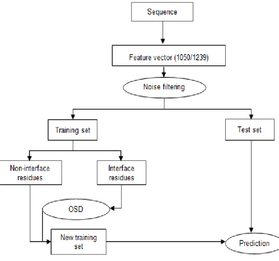
Figure 4.1 The general scheme of our method ... 50

Figure 4.2 ROC curves for the comparison of various feature groups, without feature selection on the BT426, BT547 and BT823 datasets. ... 52

Figure 4.3 R OC curves of KLR and our method on the BT426 dataset. ... 53

Figure 4.4 R OC curves on BT547 and BT823 datasets. ... 54

Figure 4.5 ROC curves of our method on the three datasets BT426, BT547, and BT823. ... 57

(11)

viii

List of Tables

Table 1.1 Kinds of tight turns in protein ... 10 Table 1.2 Average values of dihedral angles of beta-turn types. ... 11 Table 2.1 A taxonomy of feature selection techniques ... 25 Table 3.1 Performance measures comparison of different methods on the dataset D1050 in terms of best G-mean ... 37 Table 3.2 Performance of KSVM-THR-only, OSD-THR, RUS-THR and RUS-OSD-THR with different decision threshold values on the dataset D1050 ... 38 Table 3.3 Performance of KSVM-THR-only, OSD-THR, RUS-THR and RUS-OSD-THR with different decision threshold values on the dataset D1239 ... 43 Table 3.4 Performance measures comparison of different methods on the dataset D1239 ... 44 Table 3.5 Performance measures comparison on the datasets D1239 and D1050 .... 44 Table 4.1 The type turn’s distributions (%) in the datasets ... 47 Table 4.2 The evaluation results of using different window sizes for PSSM values and predicted protein blocks without under-sampling and feature selection on the BT426 dataset... 51 Table 4.3 The evaluation results of the three datasets using different kinds of feature groups with sliding window size of 9, without under-sampling and feature selection ... 53 Table 4.4 Comparison of competitive methods on the BT426 dataset. ... 54 Table 4.5 Comparison of competitive methods on the BT547 and BT823 datasets. 55 Table 4.6 Beta-turn types predicting results of our method on the BT426, BT547 and BT823 datasets ... 56 Table 4.7 MCCs comparison between the competitive methods.. ... 56

(12)

1

Chapter 1 Introduction

In this chapter, we introduce some basic concepts related to our methods in the next chapters, such as protein structure levels, torsion angles, protein blocks, -turn, and so on. After that, we briefly present some concepts and research problems of protein-protein interaction sites and -turns and their types prediction. And then, class-imbalance problem, one of the difficulties in predicting protein-protein interaction site and -turn is introduced. Dealing with these problems is our purpose.

Finally, we show the contributions and organization of our thesis.

(13)

2

1.1 Introduction

1.1.1 Protein overview Protein

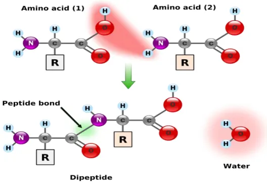
Proteins are cellular large molecules that are constructed from chains of hundreds or thousands amino acids. Each chain is called a polypeptide. Each individual amino acid in this chain is called a residue. Two amino acids link together through the peptide bond.

There are 20 amino acids that most commonly occur in nature. All of them consist of the same part, but the side chain R, as in Figure 1.1

Figure 1.2 presents the way that two amino acids link together to form a dipeptide in a protein chain.

Figure 1.1 Basic structure of amino acid.

The different amino acids have the different side-chain R. (Figure adapted from http://sph.bu.edu/otlt/MPH-Modules/PH/PH709_A_Cellular_World/PH709_A_Cellular_World6.html)

Proteins play a very important role in the cells of living organisms. Each protein has a specific function, for example, enzymes catalyze the metabolic reactions;

structural protein involves in creating the cell wall; regulatory proteins regulate the transcription of genes; transport proteins bring molecules traveling through the body;

antibodies help to protect the body by binding to the specific foreign invaders such as bacteria or viruses, and so on.

(14)

3

Most proteins interact with the other molecules to perform their function. If the interactions between proteins in a cell disappear, the cell will be blind, deaf, paralytic and disintegrate.

Figure 1.2 The condensation of two amino acids to form a dipeptide. (Figure adapted from ttp://en.wikibooks.org/wiki/An_Introduction_to_Molecular_Biology/Function_and_structure_of_Protei ns)

Figure 1.3 presents an example of antibody Immunoglobulin G traveling in the blood and protecting the body by binding with the invaders.

Figure 1.3 Antibody Immunoglobulin G recognizes foreign particles that might be harmful to defend the body.

(Figure downloaded from http://ghr.nlm.nih.gov/handbook/howgeneswork/protein)

(15)

4

Functions of proteins directly depend on their structure and shape. Protein structure can be presented as four levels (Figure 1.4):

 The primary structure is a linear amino acid sequence.

 Secondary structure refers to the local spatial arrangement of a polypeptide’s backbone atoms without regard to the conformations of its side chains.

 Tertiary structure is the three-dimensional structure of an entire protein sequence.

 Some proteins contain more than one polypeptide chain. In this case, quaternary structure of a protein is the arrangement of the three-dimensional polypeptides.

Figure 1.4 Four levels of protein structure.

a) Primary structure is a sequence of amino acids.

b) Secondary structure is the spatial arrangement of the specific regions.

c) Tertiary structure is the 3D structure of the whole polypeptide chain.

d) Quaternary structure, if exists, is the 3D structure of many polypeptide chains.

a)

c) d)

b)

(16)

5

Torsion angles

The backbone (main chain) of a protein includes the atoms which participate in the peptide bonds. It can be displayed as a linked sequence of rigid planar peptide groups and described by the torsion angles (dihedral angles)  and .  is the angle between two adjacent planes (CNC) and (NCC); and  is the angle between the planes (NCC) and (CCN) (Figure 1.5). These two angles are defined as 180 if the polypeptide sequence is fully extended conformation. Torsion angles are among the most important local structural parameters that control protein folding. If we know the values of these angles, we would be able to predict the corresponding protein 3D structure.

Figure 1.5 Torsion angles  and  of the polypeptide backbone Figure adapted from http://wiki.christophchamp.com/index.php/Ramachandran_plot

Protein blocks

Secondary structure of protein is very important for fold recognition. Secondary structures have been classically described into three states of backbone conformation as -helix, -sheet and coil. Around 50% of total number protein residues are assigned as coils. Meanwhile, these residues actually correspond to many distinct local protein structures. Therefore, a new view of three-dimensional protein structure that combines the small local fragments (or prototypes) has been developed. A structural alphabet (SA) is a complete set of these prototypes [1].

(17)

6

Because each residue relates to one of the fragments in a SA, a protein primary structure can be translated into a chain of prototypes in one dimension as the sequence of prototypes [2].

Many structural alphabets were developed, such as Building Blocks, Recurrent local structural motifs, Substructures, Structural Building Blocks, Oligons, Protein Blocks, LSP, Kappa-alpha, and so on. The more details can be found in [1].

Protein Blocks (PBs) [3] that allows a good approximation of local protein 3D structures [4] and has been applied to many applications at the present time [2, 5].

This SA is composed of sixteen local structure prototypes of five consecutive C, called Protein Blocks (PBs), labeled a, b, c, d, e, f, g, h, i, j, k, l, m, n, o, p, respectively. Each of these prototypes represents a vector of eight average dihedral angles /. Figure 1.6 displays these kinds of blocks.

Figure 1.6 The protein blocks.

For each protein block, the N-cap extremity is shown on the left and the C-cap on the right. Each prototype is five residues in length and corresponds to eight dihedral angles (φ,ψ). The protein blocks m and d are mainly associated to the central region of α-helix and the central region of β-strand, respectively [2]

(18)

7

1.1.2 Protein-protein interaction sites prediction

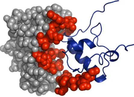
Protein-protein interactions play a major role in maintaining normal cell functions and physiology [6]. Specifically, they are responsible for many important biological processes, such as metabolic control, DNA replication, protein synthesis, immunological recognition, and so forth. Thus, studying of protein-protein interaction is a vital task in bioinformatics. This realm contains two main goals, recognizing the interaction sites (or protein interfaces) where proteins physically contact, and predicting which pairs of proteins can interact. The knowledge of protein interfaces allows us to understand the way protein recognizes the other molecules and engineers new interactions. It is also very useful in identifying drug targets, designing drug-like peptides to prevent unwanted interactions [7, 8]. The demonstration of the interaction sites of two protein sequences is presented in Figure 1.7.

There are many experimental methods to identify the protein interaction sites and interface residues, such as X-ray Crystallography, Nuclear magnetic resonance [9] or Site-specific mutagenesis [10]. However, these approaches are expensive, time-consuming and problematic for transient complexes [11], while computational methods are more cost-effective.

Predicting protein-protein interaction sites by machine learning methods can be dealt as a classification problem that to predict whether an amino acid is an interface residue or not. The features that can distinguish interaction and non-interaction residues are used to describe protein site [11].

There are two main groups of methods for predicting protein-protein interaction sites, the methods using protein structure and the methods using protein sequence information [12].

The protein structure based methods represent each residue by information of its nearest neighbors in structure [13–15], thus they can utilize the informative features.

However, the number of known-structure proteins to date is significantly smaller than the amount of protein sequences [16]. Therefore, it is necessary to develop the methods that can predict the interface residues from the amino acid sequence only, without knowing structural information. These methods generally generate the features for each residue from information of it and its neighbors in the sequence.

Some studies have attempted to develop the techniques for predicting interaction

(19)

8

sites from protein sequences. For example, Kini and Evans [17] relied on the most common appearance of proline in the flanking segments of interaction sites to propose the prediction method; Chen and Li [18] combined the hydrophobic and evolutionary information of amino acid to construct the prediction model; Chen and Jeong [16]

extracted a wide range of features from protein sequences only and using Random Forests to create a prediction integrative model, and so forth.

However, it is not easy to apply sequence-based methods for interaction sites prediction due to the lack of understanding of biological properties that can provide vital information related to binding sites. Ofran and Rost [19, 20] proved that using better information would induce better prediction results. On the other hand, because the number of non-interacting residues is much more than the number of interacting residues, it often leads to the high value of false predicted negative.

Figure 1.7 Illustration of protein-protein interaction interface residues of sequence 1FJG-F and ribosomal subunit S18.

Reds denote the interface residues.

(Figure adapted from http://www.insun.hit.edu.cn/~mhli/site_CRFs/fig/1FJG_F_right_1024.png)

(20)

9

1.1.3 -turn prediction

There is a tight relationship between a protein sequence, structure, and its function.

The understanding of structural basis for protein function can speed up the progress in systems biology that aims at identifying functional networks of proteins. For example, the rational drug design heavily relies on the structural knowledge of a protein [6].

Secondary structure, that includes regular and irregular patterns, is very important in protein folding study since it can provide the useful information to derive the possible three-dimensional structures. The regular structures, composed of sequences of residues with repeating  and  values, classified in -helix and -strand. While this class is well defined, the other class, irregular structures, involves 50% of remaining protein residues are classified as coils. In fact, coil can be tight turn, bulge or random coil. Among of these structures, tight turn is the most important from the viewpoint of structure as well as function [21].

Tight turns are categorized into -turn, -turn, -turn, -turn and -turn basing on the number of consecutive residues in the turn. Table 1.1 displays the kinds of tight turns.

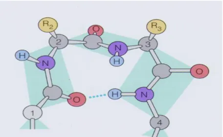
-turn is one of the most common tight turns. A -turn is composed of four consecutive residues that are not in an -helix and the distance between the first and the fourth C is less than 7Å [22] (Figure 1.8). -turns play an important role in the conformation as well as the function of protein, and make up around 25% of the residue numbers. -turns are the essential part of -hairpins, provide the directional change of the polypeptide [23], and involve in the molecular recognition processes [24]. In addition, the formation of -turn is a vital step in protein folding [25].

Therefore, the knowledge of -turn is very necessary in the prediction of three-dimensional structure of a given primary protein sequence.

(21)

10

Figure 1.8 An example of beta-turn that contains four consecutive residues.

The C- are numbered from 1 to 4. Dot line represents hydrogen bond

Table 1.1 Kinds of tight turns in protein

Type No. of residues H-bonding

-turn 2 NH(i)-CO(i+1)

-turn 3 CO(i)-NH(i+2)

-turn 4 CO(i)-NH(i+3)

-turn 5 CO(i)-NH(i+4)

-turn 6 CO(i)-NH(i+5)

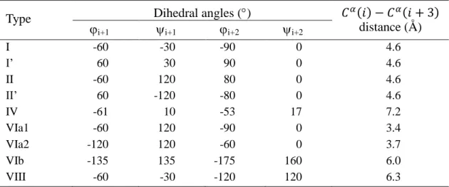
-turns are categorized into nine types (I, I’, II, II’, IV, VIa1, VIa2, VIb and VIII) based on the dihedral angles of residues i+1 and i+2 in the turn [26]. The detailed values of these angles corresponding to each type are shown in Table 1.2. Because the turn types VIa1, VIa2 and VIb are rare, they are often combined into one type and named VI [21]. Figure 1.9 below displays the illustrative drawings of nine -turn types.

The -turn prediction methods can be divided into two main categories: statistical techniques and machine learning techniques. The former group includes the techniques such as Chou-Fasman’s method [27], Thornton’s methods [28, 29], Chou’s method [30], the 1-4 and 2-3 correlation model [31] using the positional frequencies and -turn residue conformation parameters; and the more recently method COUDES

(22)

11

[32], that used the propensities and multiple sequence alignments.

The latter group was reported to be effectively applied for -turns prediction in recent years [33]. Belonging to this realm, Artificial Neural Network (ANN) was first used in [34], then frequently used by the other authors [22, 35, 36]. Support Vector Machines (SVMs) were also selected by many authors [24, 33, 37–41]. The most recent reported result is KLR, which used kernel logistic regression for prediction, with 0.5 on Matthews correlation coefficient (MCC) [42].

Most of the methods for the turn types prediction are based on ANN [35, 43, 44]

or probabilities with multiple sequence alignments as COUDES [32]. More recently, Kountouris and Hirst [33] and X.Shi [45] used SVM in their methods and achieved the significant results. However, the quality of both -turn location and turn types prediction is a challenge.

Table 1.2 Average values of dihedral angles of beta-turn types.

The third residue of turns type VIa1,VIa2, VIb must be a proline [21, 26]

Type Dihedral angles ()

distance (Å)

i+1 i+1 i+2 i+2

I -60 -30 -90 0 4.6

I’ 60 30 90 0 4.6

II -60 120 80 0 4.6

II’ 60 -120 -80 0 4.6

IV -61 10 -53 17 7.2

VIa1 -60 120 -90 0 3.4

VIa2 -120 120 -60 0 3.7

VIb -135 135 -175 160 6.0

VIII -60 -30 -120 120 6.3

(23)

12

Figure 1.9 Illustrative stereo drawings of beta-turn types.

The distances between C_α(i)-C_α(i+3) in type IV are slightly greater than 7Å since this type is a miscellaneous category and not really considered as an authentic -turn [21]

.

1.1.4 Class-imbalance problems

In recent years, class-imbalance problems have been receiving many deep concerns because of their importance. A dataset is imbalanced if the number of samples in some classes is significantly larger than in other classes. In the case of two-class datasets, the class with small amount of samples is the minority (positive) class while the other is the majority (negative) class. For multi-class imbalanced datasets, there can be some minority classes, and in some situations, every class is the minority. However, in this thesis, we just focus on the two-class problem to agree with the common practices [46–50]. Figure 1.10 presents an illustration of imbalanced dataset.The class-imbalance problem is often found in the real decision systems which try to detect the rare but important cases such as fraud detection [51, 52], oil spills in

(24)

13

satellite images of the sea surface [53], risk management [54], text categorization [55]

and so on. In the field of bioinformatics, this problem is very common, such as miRNA prediction [56], beta-turns prediction [33, 42], prediction of protein-interaction sites [16, 57, 58], protein-ATP binding residues prediction [59], microRNAs classification [60–62], translation initiation site recognition [63], et cetera.

In some cases, the ratio of minority class to majority class can be as extreme as 1:100 or 1:100,000 [46]. When applying standard machine learning to the such datasets, it often harvests a poor performance that results from the accuracy. Most of the learning systems can be seriously influenced and tend to predict majority class exactly while users desire for both high sensitivity and specificity. One of the most common examples in real biomedical applications is the “Mammography Data Set,” the collection of images acquired from a series of mammography exams performed on a set of distinct patients. Analyzing the images in a binary sense, the natural classes are labeled “Positive” for an image representative of a “healthy”, and “Negative” for a

“cancerous” patient. This data set contains 10,923 “Negative” samples and 260

“Positive” samples. We expect a classifier will provide 100% of predictive accuracy for both the minority and majority classes on the dataset. However, the reality showed that classifiers tend to provide a severe imbalanced degree of accuracy, with the majority class having close to 100% accuracy and the minority class having accuracies of 0-10 percent. If a classifier achieves 10% accuracy on the minority class of the mammography data set, it means that 234 minority samples are misclassified as majority samples. The consequence of this is equivalent to 234 cancerous patients diagnosed as noncancerous. This is clearly an undesired result [46].

In addition, class distribution and error costs also affect the learning algorithms.

Standard classifiers assume that (i) the algorithms will perform on data drawn from the same distribution as the training data while the training and testing distributions are often different; (ii) the errors coming from different classes have the same costs while they are unlike in practice [64].

To solve this problem, many strategies have been proposed. Basically, all of them are divided into two categories: data level including the resampling methods, and algorithmic level including the methods aiming at adjusting the parameters of machine learning algorithms [46, 49]. However, [46] shows that resampling techniques are more effective on improving classifier accuracy than algorithm level

(25)

14

methods. Due to that reason, in this study, we mainly focus on the resampling techniques.

Figure 1.10 An illustration of an imbalanced dataset.

Blackened shapes represent samples; circles are majority class samples and stars are minority class samples.

1.2 Objectives

Because of the importance of predicting the interface residue and -turn and what kind of turn it is, our thesis aims to the following problems:

Firstly, we would like to improve the performance of predicting protein interface residue by solving the problem of class-imbalance. To do that, we propose a new over-sampling algorithm for balancing the dataset. We chose the dataset that contains 2,829 interacting residues and 24,616 non-interacting residues for training and testing the predictor, and compare our results with the state-of-the-art approaches. We also combine our algorithm with some other methods to enhance the better results.

In addition, we try to use a new kind of feature for well distinguishing the protein interface and non-interface residues. We apply our new algorithm to this new dataset to evaluate the performance.

Secondly, we would like to better the quality of predicting -turn . Since the high proportion of non--turn residues to the -turn residues is one of the reasons decreasing the prediction’s performance, we utilize random under-sampling method to balance the dataset. We create the well-characterized datasets for training and testing the model. We also apply this idea for predicting -turn types. The results are compared with other state-of-the-art methods to evaluate the improvement.

(26)

15

1.3 Contributions

The main contributions of this thesis are described as below:

A novel over-sampling technique for relaxing the class-imbalance problem based on local density distributions. In order to alleviate the problem of overlapping and over-fitting simultaneously, we propose a novel over-sampling algorithm, which we name Over-sampling based on local Density (OSD). OSD algorithm focuses on only minority samples located where the local density of minority samples is small in comparison with that of majority samples. As the local minority density is smaller, OSD increases the number of minority samples more strongly by synthesizing artificial minority samples.

The enhancement on the performance of predicting protein-protein interaction sites by using our new over-sampling method OSD. We also proposed the methods combined with KSVM-THR and random under-sampling methods to reinforce the tolerance for the class imbalance problem. Results from experiments showed that the combination of our OSD algorithm and new feature group led to high sensitivity, precision, G-mean, MCC, F-measure, and AUC-PR, and comparable performance with the state-of-the-art methods. In addition, we found that the information of predicted shape strings increased the performance for predicting whether interface or non-interface residues.

The improvement in the performance of predicting -turns and their types.

We utilize predicted protein blocks and position specific scoring matrix together with random under-sampling method to improve the predicting the -turns and their types.

We executed the experiments on three benchmark datasets, and achieved MCCs of 0.58, 0.59 and 0.58 on the three datasets BT426, BT547 and BT823, respectively, in comparison of the state-of-art -turn prediction methods. In the field of -turn types prediction, we also harvested the high and stable results.

1.4 Thesis Organization

This thesis includes five chapters.

(27)

16

The first chapter is the current one that gives the basic concepts such as protein structure levels, protein blocks and the brief introduction of our research topic, thesis contributions and organization.

Chapter 2 introduces the overview of techniques for dealing with class-imbalance problems and evaluation metrics for imbalanced datasets classification.

Chapter 3 describes the improvement in predicting protein-protein interaction sites by using a novel over-sampling method and predicted shape strings.

Chapter 4 presents the improvement in the prediction of -turns and their types applying predicted protein blocks and under-sampling method.

Chapter 5 concludes this thesis and mentions the future works.

(28)

17

Chapter 2 Methods for Dealing with Class-imbalance Problems

The methods to handle the class-imbalance problem are categorized into two groups, data-level methods and algorithm-level methods. This chapter aims to present briefly the methods that have been used to deal with this problem. Then, the performance evaluation measures such as overall accuracy, G-mean, Mathews Correlation Coefficient, and so on, which are often utilized to evaluate the classification performance on the imbalanced datasets are presented.

(29)

18

2.1 Standard Classifier Modeling Algorithm

There are many basic well-known classifier learning algorithms such as K-nearest Neighbors [65], Decision trees (ID3 [66], C4.5 [67]), Back-propagation Neural Networks [68], Support Vector Machines [69], and so forth. Due to the limitation of space, in this thesis, we just focus on Support Vector Machines that are mainly used for our research.

Support Vector Machines (SVMs), a popular machine learning technique, which have been successfully applied to many real-world classification problems from various domains, were proposed by Vapnik.

The goal of the SVM learning algorithm is finding the optimal hyper-plane to separate the dataset into two classes, with the maximal margin. Here, margin is the minimal distance from the hyper-plane to the closest data points. The solution is based only on the support vectors, which are the data points at the margin. SVMs originally were for the linear binary classification problem. However, in many applications, the linear classifier cannot work well but the non-linear classifier. In these cases, the non-linear separated problem is transformed into a high dimensional feature space using a set of non-linear basis functions. An important property of SVMs is that it is not necessary to know the mapping function explicitly. A kernel representation by a kernel function can be used, instead. When perfect separation is not possible, slack variables are introduced for sample vectors to balance the trade-off between maximizing the width of the margin and minimizing the associated error [48].

SVMs are believed to be less affected by the class imbalance problem than other classification learning algorithms [70] since boundaries between classes are calculated based on the support vectors and the class sizes may not affect the class boundary too much. However, some weaknesses of SVMs when applying to the imbalanced datasets were reported. [71] showed that in this case, the separating hyper-plane of an SVM model can be skewed towards the minority class, therefore can degrade the performance of the model with respect to the minority class. Wu and Chang [72]

reported when the dataset is unbalanced, the positive samples lie further from the ideal boundary result in the boundary skew. They also said that in this case, the ratio

(30)

19

of positive and negative support vectors would be imbalanced. However, the authors in [73] objected to this idea.

2.2 The State-of-the-art Solutions for Class-imbalance Problems

2.2.1 Resampling techniques

Generally, resampling techniques aim to balance the distribution of the dataset by some mechanisms. This group includes the methods such as over-sampling the minority class, under-sampling the majority class, and combinations of the above techniques.

Over-sampling

Over-sampling method tries to balance the data set by increasing the number of minority class samples.

The simplest way is named Random Over-sampling, which randomly chooses some minority samples, replicates them and then adds to the original dataset.

However, this strategy can lead to the over-fitting since over-sampling simply appends duplicated samples to the original data set, multiple instances of certain samples become “tied” [49, 74]. In addition, in case of large data sets, the cost in time and memory of classifying phase will be increased [46, 49].

Related synthetic sampling, the Synthetic Minority Over-sampling TEchnique (SMOTE) [75] is a powerful method that has been successfully applied for many research [76]. SMOTE tries to overcome the over-fitting by generating synthetic samples between each minority class instance and its randomly selected nearest neighbors. The synthetic sample x_new of a minority sample x_i is created by

where δ is a random number in [0,1] and xn is one of the k nearest neighbors of xi. Figure 2.1 presents an example of SMOTE.

(31)

20 Figure 2.1 An illustration of SMOTE algorithm.

Dataset with majority class samples (circles) and minority class samples (stars). Minority sample x_i(in red) and its five nearest neighbors (in blue). The synthetic sample which is generated by x_i and one of its random chosen nearest neighbor is presented as the blue square.

Though SMOTE can overcome the drawback of Random Over-sampling, the numbers of synthetic samples corresponding to each minority class instance are the same may result in the overlapping between classes. Many improvements of SMOTE, therefore, were developed, such as SMOTEBoost [77], Smote-RSB [78], Safe-Level-SMOTE [79], Borderline-SMOTE [80] and so on.

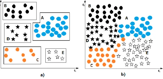
The other over-sampling methods that need to pay attention to are the Cluster-based sampling algorithms. These methods are more flexible than the simple and synthetic sampling algorithms, and can be tailored to target very specific problems. CBO, the cluster-based over-sampling algorithm [81], effectively deals with the within-class imbalance problem [46]. The basic idea of this method is clustering before over-sampling. Specifically, in [81], the authors used K-mean to cluster the whole dataset. Then, both the minority class and majority class were oversampled. All the clusters in the majority class were randomly oversampled but the largest one. After this step, every majority cluster had the same size. In the minority class, each cluster was oversampled so that it would contain maxsize/nclusters samples, where maxsize was the overall size of the majority class after over-sampling, and nclusters was the number of minority clusters. The illustrative example of this method is in Figure 2.2 [46].

(32)

21

Figure 2.2 Cluster-Based Sampling method example.

a) Dataset with three majority clusters (A, B, C) and two minority clusters (D, E). Cluster A contains the most number of samples.

b) After applying the method, every cluster contains the same number of samples as cluster A.

Under-sampling

Contrary to Over-sampling, Under-sampling method solves the class-imbalance problem by decreasing the number of majority class samples, therefore, decreases the cost of computation.

Random Under-sampling balances the original data set distribution by randomly eliminating some majority samples. However, this way may lead to lose a lot of important information of the majority class.

EasyEnsemble, BalanceCascade [82] were proposed to overcome this limitation.

EasyEnsemble develops an ensemble learning system by independently sampling several subsets from the majority class and developing multiple classifiers based on the combination of each subset with the minority class samples. On the other hand, the BalanceCascade develops an ensemble of classifiers to select which majority class samples for under-sampling systematically.

The other under-sampling methods that based on k-nearest neighbors are NearMiss-1, NearMiss-2, Near-Miss-3, and the “most distant” method [50]. The NearMiss-1 method chooses majority samples whose average distance to the three minority class nearest neighbors is the smallest. The NearMiss-2 method selects the majority class samples whose average distance to the three farthest minority class

(33)

22

neighbors is the smallest. NearMiss-3 selects a given number of majority class samples that are closest to each minority sample to guarantee that every minoritysample is surrounded by some majority examples. The “most distance”

method selects the majority class samples whose average distance to the three minority class nearest neighbors is the largest.

Anand et al. [61] introduced an under-sampling method that also based on nearest neighbor and weighted SVM. For each minority class sample, its k closest majority class samples will be removed. The distance between samples here is weighted Euclidean distance.

2.2.2 Algorithm level methods for handling imbalance

This group of methods modifies the standard classification algorithm to account for class-imbalance. A popular way for dealing with the class-imbalance problem is to choose a proper inductive bias. For decision trees, approaches are adjusting the probabilistic estimate at the tree leaf [83, 84] or developing new pruning techniques [83].

For SVMs, the use of different penalty constants for different classes (cost-sensitive) [73, 85, 86], and adjusting the class boundary based on kernel-alignment ideal [72] were proposed.

Cost-sensitive learning methods deal with the class-imbalance problem by considering the costs associated with misclassifying samples [87, 88]. One of the simple ways is adjusting the decision threshold in assigning class memberships. Chen et al. [89] shows that the adjustment decision threshold can increase the sensitivity and decrease specificity via the experiments on for four classification algorithms:

logistic regression model, classification tree, Fisher’s linear discriminant and modified nearest neighbor. Using the same idea, Lin and Chen [90] proposed the SVM-THR method that adjusted the decision threshold of SVM. These methods are said to be naturally applied to handle the imbalanced datasets [46].

The other strategy is one-class learning method. The one-class learning approach learns on only one class to determine the decision boundary [91, 92]. Raskutti and Kowalczyk [93] demonstrates that one-class learning method performs well for extreme imbalanced datasets composed of a high dimensional noisy feature space.

(34)

23

One drawback of these methods is the requirement of the algorithm-specific modification.

2.3 Feature Selection for Imbalance Datasets

Feature selection is a pre-processing technique that to select a subset of best features.

The purpose of feature selection is to avoid over-fitting and improve model’s performance, to provide a cost-effective model, and to gain a deeper insight into the underlying processes that generated the data [94]. In the field of imbalanced datasets mining, feature selection is even more important than the choice of the learning method [64, 95].

The general feature selection process is described as follow:

A feature selection algorithm belongs to one of three groups: filter methods, wrapper methods, and embed methods.

Filter method selects the features based on their relevance scores. The relevance scores of features are calculated by various feature-ranking techniques such as Euclidean distance, Chi-squared, Information Gain, Gain Ratio, Symmetric Uncertainty, ReliefF, and so on [96]. These methods are fast, easily scale for high dimensional datasets, independent of the classification algorithm but ignoring the

Feature selection algorithm Training set

Selected feature subset

Test set Final evaluation

Output performance

(35)

24

interaction with classifier [94]. The general scheme of filter method description is in Figure 2.3.

Wrapper methods (Figure 2.4), such as Sequential forward selection technique, Sequential backward selection technique, SVM-RFE, ect., use the classifier to calculate the score of feature-subsets based on their predictive power. These methods pay attention to the feature dependencies and interact with the classifier. However, the common drawback is that they are computationally intensive and have high risk of overfitting [94, 97].

The embedded methods can be seen as the hybrid methods with the combination of filter and wrapper methods. Firstly, filter model is applied to identify the goodness of features. Then, a wrapper model is performed to choose the optimal feature-subset.

Table 2.1 from [94] presents the taxonomy of feature selection techniques.

Dimension Reduced Training

Set Machine Learning Algorithm

Training Set

Feature Set Feature Merit

Feature Search

Feature Evaluate

Estimated Accuracy Final Evaluation

Hypothesis

Dimension Reduced Test Set Figure 2.3 Filter method.Figure adapted from [97]

(36)

25

Table 2.1 A taxonomy of feature selection techniques [94]

Model search Advantages Disadvantages Examples

Filter

(Uni-variate)

 Fast

 Scalable

 Independent of the classifier

 Ignores feature dependencies

 Ignore interation with the classifier

 Chi-squared

 Euclidean distance

 t-test

 Information gain, Gain ratio

Filter

(Multivariate)

 Models feature dependencies

 Independent of the classifier

 Better

computational complexity than wrapper methods

 Slower than

univariate techniques

 Less scalable than univariate techniques

 Ignores interaction with the classifier

 Correlation-based feature selection (CFS)

 Markov blanket filter

 Fast

correlation-based feature selection (FCBF)

Wrapper (Deterministic)

 Simple

 Interacts with the classifier

 Less

computationally

 Intensive than randomized methods

 Risk of over fitting

 More prone than randomized

algorithms to getting stuck in a local optimum (greedy search)

 Classifier dependent selection

 Sequential forward selection (SFS)

 Sequential backward

elimination (SBE)

 Plus q take-away r

 Beam search

Wrapper (Randomized)

 Less prone to local optima

 Computationally intensive

 Higher risk of over-fitting than deterministic algorithms

 Simulated annealing

 Randomized hill climbing

 Genetic algorithms

 Estimation of distribution algorithms

Embedded

 Better

computational complexity than wrapper methods

 Decision trees

 Weighted naïve Bayes

 Feature selection using the weight vector of SVM

(37)

26

Figure 2.4 Wrapper method. Figure adapted from [98]

2.4 Evaluation Metrics

Evaluation measures aim to evaluate the classification performance and to guide the classifier modeling. For the normal situation, overall accuracy is often used. However, when performing the classification on the imbalanced datasets, overall accuracy is no longer suitable for evaluating the performance of classifier [99]. If the class-imbalance problem is severe, a naive approach will make the overall accuracy very high even though, most samples are assigned to the majority class and no sample is assigned to the minority class [46].

Thus, besides overall accuracy, in this study, the other metrics such as sensitivity, specificity, G-mean, F-measure and Matthews correlation coefficient are used, which are defined as follows:

Overall accuracy = Sensitivity = Recall =

Feature Set

Feature Selection Search Performance Estimation

Induction Algorithm Hypothesis

Training Set

Estimated Accuracy Final

Evaluation Test Set

Feature Set

Induction Algorithm

Feature Set

Feature Evaluation