TakeshiKudo FiscalConsolidationandSustainabilityofJapan ʼ sPublicDebtaftertheGlobalFinancialCrisis

Abstract

After the ２００８ global financial crisis, the sustainability of public indebtedness has become a central public policy issue in the United States, Europe, and Japan. In the United States especially, the pub- lic debt ceiling has become a continuing source of concern and politi- cal dispute. This paper employs Japanese Long-term Economic Sta- tistics （LTES） to investigate the sustainability of Japanʼs public debt and changes in fiscal discipline after the ２００８ global financial crisis.

First, results of the unit-root test show that the level of Japanʼs public debt has become unsustainable after the crisis. Second, the ２００８ global financial crisis has destroyed Japanʼs fiscal discipline, which had been relatively strong before the crisis. Third, fiscal disci- pline was strong between the Russo‒Japanese War and World War I and for several decades following World War II. It was relatively strong during the fiscal consolidation period in the latter １９８０ s. We thus conclude that post-war fiscal discipline in Japan resembled the pre-war period despite the absence of military expenses after World War II. Although fiscal consolidation could reduce public debt to some degree, the level of public debt in ２０１７ might generate high in- flation in the future, as it did after World Wars I and II.

Keywords : Public debt, fiscal deficit, Sustainability of the public debt

Fiscal Consolidation and Sustainability of Japan ʼ s Public Debt after the Global Financial Crisis

Takeshi Kudo

１）Shaded areas indicate wartime. These include the First Sino‒Japanese War

（１８９４‒１８９５） , the Russo‒Japanese War（１９０３‒１９０７） , World War I including the Siberian Intervention（１９１４‒１９２０） , and the Second Sino‒Japanese War and Pa- cific Ocean War（１９３７‒１９４５） . These periods are defined as the fiscal years in which government implemented the Extraordinary Special Accounts for War Expenses.

Data Sources）

•１８８５‒２００２ : Statistics Bureau, Ministry of Internal Affairs and Communications, Historical Statistics of Japan, Table ５‒９ .

•２００３‒２０１７ : Ministry of Finance

Figure １: Public Debt in Japan

１ Introduction

Tax reductions and increased public expenditure during the long-term stagnation since the １９９０ s resulted in Japanʼs public debt approaching ２００％ of its GDP at the end of ２０１０ . Japanʼs debt has soared since the global financial crisis in late ２００８ . The debt‒GDP ratio increased by １８％

in ２００９ . People are worried about the debt because Japan ʼ s labor power has decreased through a falling birth rate and aging society.

The Japanese economy has never experienced rapid debt accumula-

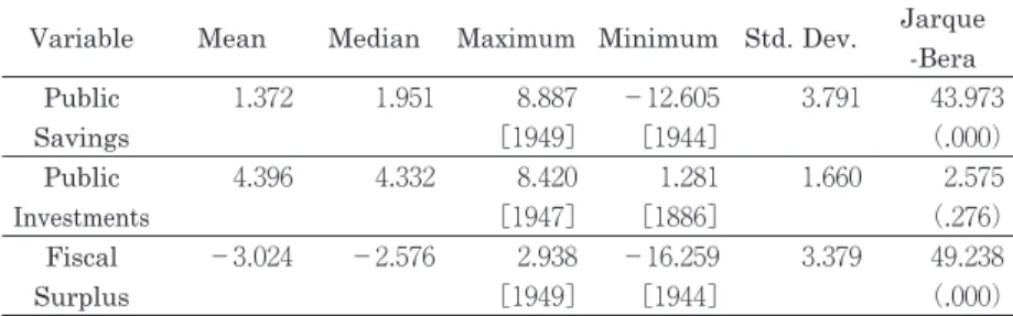
１）Shaded areas indicate wartime. These include the First Sino‒Japanese War

（１８９４‒１８９５） , the Russo‒Japanese War（１９０３‒１９０７） , World War I including the Siberian Intervention（１９１４‒１９２０） , and the Second Sino‒Japanese War and the Pacific Ocean War（１９３７‒１９４５） . These periods are defined as the fiscal years in which government implemented the Extraordinary Special Accounts for War Expenses.

Data Sources）

•１８８５‒１９４０ : Ohkawa and Shinohara（１９７９）

•１９４１‒１９５５ : Japan Statistical Association（１９８８）

•１９５５‒１９７９ : Cabinet Office, National Accounts for １９９８.

•１９８０‒１９９３ : Cabinet Office, National Accounts for ２００９.

•１９９４‒２０１７ : Cabinet Office, National Accounts for ２０１７.

Figure ２: Fiscal Surpluses（General Government）in Japan

tion. After the Russo‒Japanese War（１９０４‒１９０５） , government financed huge war expenses by issuing government bonds. Other examples of long-term war expenses include the Second Sino‒Japanese War and the Pacific Ocean War from １９３７to １９４５（Figure １） .

Each example above involves different processes of adjusting public

debt. Public debt associated with the Russo‒Japanese War was resolved

by fiscal surpluses after the war. Debt accumulated between １９３７ and

１ Doi et al. （２００５） and Iwamura et al. （２００６） conclude that the public debt is not sustainable, while Broda and Weinstein（２００５） simulate certain cases using the data and conclude that it is sustainable.

２ Leeper（１９９１）calls this situation an “active” fiscal policy, and Woodford

（１９９５）subsequently defines it as a “Non-Ricardian” fiscal policy.

１９４５was reduced by hyperinflation after the war（Figures ２ and ３） . Our analysis considers the following aspects. First, we verify the sus- tainability of Japanʼs public debt by using Long-term Economic Statis- tics（LTES）since the １８８０ s. Ahmed and Rogers（１９９５）examined long- term data in the U.S. and UK and concluded that these nationsʼ public indebtedness is sustainable. In Japan, research using long-term histori- cal data is rare, although Broda and Weinstein（２００５） , Doi et al. （２００５） , and Iwamura et al. （２００６）used data from the post-war period.

Second, we implement the Markov-switching regression to consider the possibility of structural breaks after events such as the ２００８ global financial crisis. Okazaki（２００４）shows that fiscal discipline has relaxed since the end of １９２０ s. We investigate whether this structural change is observed in actual data.

Besides these empirical issues, tests with structural breaks are impor- tant. Sustainability is defined as the case in which the ex-post inter- temporal budget constraint is satisfied. This definition allows a reduc- tion in the value of debt resulting from hyperinflation associated with fiscal collapse.

Therefore, tests that reveal structural breaks enable us to investigate the sustainability of public debt even when the sustain- ability condition is temporarily not satisfied.

The rest of this paper is organized as follows. Section ２ reviews re-

lated research to examine the conditions for fiscal sustainability. Section

３ implements tests for the sustainability of public debt using LTES on

１）The shaded areas indicate wartime periods. These include the First Sino‒

Japanese War（１８９４‒１８９５） , the Russo‒Japanese War（１９０３‒１９０７） , World War I including the Siberian Intervention（１９１４‒１９２０） , and the Second Sino‒Japa- nese War and the Pacific Ocean War（１９３７‒１９４５） . These periods are defined as the fiscal years in which government implemented Extraordinary Special Ac- counts for War Expenses.

２） Japan suffered hyperinflation after the Pacific Ocean War. Records show １０４ . ３

% in １９４５ , ５３５ .１ % in １９４６ , １４５ . ０ % in １９４７ , and ７７ .８ % in １９４８ . Data Sources）

•１８８５‒１９５５ : Ohkawa and Shinohara （１９７９） .

•１９５５‒１９７９ : Cabinet Office, National Accounts for １９９８.

•１９８０‒１９９３ : Cabinet Office, National Accounts for ２００９.

•１９９４‒２０１７ : Cabinet Office, National Accounts for ２０１７.

Figure ３: GDP Deflator in Japan

the basis of the methods reviewed in section ２ . Section ４ discusses fiscal

discipline in Japan alongside results from section ２ . Section ５ presents

the conclusion of the study.

２ Testing the Sustainability of Public Debt

２ . １ Testing Sustainability with a Linear Model

This study employs methods to test the sustainability of public debt;

these methods were developed by Hamilton and Flavin（１９８６） . Trehan and Walsh（１９９１）expanded their methods to include the variability of market discount rates. The necessary condition for sustainability of pub- lic debt is the cointegration of tax revenue, government expenditures, and interest on public debt; the sufficient condition is the stationarity of public debt. In that regard, Trehan and Walsh（１９９１）tested the neces- sary and sufficient conditions and concluded that the U.S. public debt is sustainable.

Bohn（１９９５）and Ahmed and Rogers（１９９５）used the necessary and sufficient conditions that tax revenue, government expenditures, and in- terest on public debt consist of a cointegration vector and that this vec- tor satisfies a constraint.

We obtain the condition for the sustainability from governmentʼs budget constraint. First, the flow budget constraint in period t is given as

（１） D

−D

＝G

−T

＋r

D

＝−s

,

where D

is the level of public debt, G

is government expenditure, T

is tax revenue, r

D

is interest on public debt, and s

is the fiscal surplus.

The stochastic discount factor is defined as Q

＝［ β

u' （ C

） /u' （ C

）］ ,

where β is the subjective discount factor, C

is the consumption level at

period t, u （·）is the utility function that satisfies the conditions u' （·） >０

and u'' （·） <０ . The Euler condition for inter-temporal substitution of con-

sumption satisfies

（２） E ［（

^"

"

Q

）］ ^{＝１ .}

Solving equation（１）and substituting equation（２）into the budget constraint, we obtain the inter-temporal budget constraint as

（３） E

!

Q

G

−E

!

"!!

"

Q

T

+ （１ +r

） D

＝lim

K→∞

E

Q

D

. We will show the condition for the sustainability of public debt. If the transversality condition for this system, lim

K→∞

E

Q

D

＝０ , is satisfied, we obtain

（４） （１＋r

） D

＝E

!

"!!

"

Q

（G

−T

） .

This means that the level of public debt at the beginning must be equal to the present value of governmentʼs present and future net reve- nue if the present value of public debt at the terminal is to converge to zero̶that is, if it is to satisfy the transversality condition.

Ahmed and Rogers（１９９５）transformed equation （３） to derive the nec- essary and sufficient condition for sustainability. Differencing and ar- ranging equation （３） , we obtain

（５） ΔE

!

"!!

"

Q

G

− ΔE

!

"!!

"

Q

T

＋（ G

− T

＋ r

D

）

＝lim

E

Q

D

−lim

K→∞

E

Q

D

,

where Δ is the difference operator.

Ahmed and Rogers（１９９５）show that the necessary and sufficient con- dition for the sustainability is that government expenditures, tax reve- nue, and interest on public debt consist of the cointegration vector （１ ,

−１ , １） . This constraint on the cointegration vector indicates the fiscal

deficit −s

in equation （１） . Therefore, we can verify the sustainability of public debt by testing the stationarity of the fiscal deficit −s

. This test is usually implemented as a unit-root test for

（６） Δs

＝μ＋λ s

＋ε

,

where the null hypothesis is λ＝０ .

２.２ Structural Breaks and Sustainability

When the true model is not linear, as in equation（６） , unit-root tests do not function because of a formulation error. Raybaudi et al. （２００４） em- ployed a nonlinear model with structural breaks between stationary and non-stationary regimes to test the sustainability of current account defi- cits by estimating the Markov-switching regression as

（７） Stationary regime （θ

＝０）：Δs

＝μ

＋λ s

＋σε

,

（８） Non stationary regime （θ

＝１）：Δs

＝μ

＋σε

.

Combining these equations, we obtain

（９） Δs

＝［μ （１−θ

）＋μ

θ

］＋λ （１−θ

） s

＋σε

,

where coefficient λ satisfies −２< λ <０ , and ε

is the disturbance term, which follows the white-noise process. The state variable θ

follows the first-order Markov chain θ∈Θ＝{ ０ , １ }, and the transition probability p

＝ P ｛θ

＝j|θ

＝i｝ satisfies p

∈［０ , １］ and ∑

p

＝１ .

The Markov-switching model is estimated by the maximum likelihood method assuming that the conditional probability density, given the ob- served and state variables till period t is Gaussian. If θ

＝１ in equation

（９） , then the process of s

follows equation （８） , and it can be concluded

that it is locally̶but not necessarily globally̶non-stationary. Francq and Zakoian （２００１） defined the necessary and sufficient condition for sec- ond-order stationarity as

（１０） x＝p

ρ

＋p

＋（１−p

−p

） ρ

< １ ,

（１１） y ＝ p

ρ

＋ p

< ２ ,

where ρ＝１＋λ.

３ Empirical Analysis Using Japanese Long-term Economic Statistics （ LTES ）

In this section, we test the sustainability of Japanʼs public debt and test for structural breaks in the data by using LTES in Japan. First, we explain the data. Second, we test the sustainability of public debt using a linear model by employing a cointegration test. Third, we test sustain- ability with a structural break by estimating the Markov-switching model. Finally, we discuss Japanʼs fiscal discipline in the context of long -term historical data.

３.１ Data

Data in our analysis concerning fiscal surpluses are calculated from SNA data. Public saving is indicated by S

, public capital formation is represented by I

, and net interest payments used in this calculation are represented as

s

＝ T

− G

− r

D

＝ S

− I

.

All data are divided by GDP.

３ These periods do not necessarily correspond to the actual war days because these periods are defined as the fiscal years in which the Extraordinary Special Accounts for War Expenses were planned and implemented by the government.

We used annual data from １８８５ to ２００９ collected from Ohkawa and Shinohara （１９７９） , the Japan Statistical Association （１９８８） , and the Cabi- net Office of Japan. We used a sequence of interest payments on govern- ment bonds until １９５４ from the Annual Reports on Government Bond Statistics because property income was unavailable in SNA data for this period.

Level shifts may occur in our data between １９４０ and １９４１ when the data estimated by Ohkawa and Shinohara（１９７９）are chained to those estimated by the Japan Statistical Association（１９８８）between １９５４ and １９５５ when the data are chained to ６８ SNA, between １９７９ and １９８０ when the data are chained to ９３ SNA, and between １９９３ and １９９４ when the data are chained to ２００８ SNA. However, information useful in testing for structural breaks may be lost by axiomatically correcting for level shifts;

hence, we do not correct data prior to analysis.

Figure ２shows the sequence of fiscal surpluses. Shaded areas indicate wartime: the First Sino‒Japanese War １８９４‒１８９５ , the Russo‒Japanese War １９０３‒１９０７ , World War I including the Siberian Intervention １９１４‒

１９２０ , and the Second Sino‒Japanese War and Pacific Ocean War（World War II）１９３７‒１９４５ .

Fiscal surpluses tend to decline in wartime, but they improved rapidly after the Russo‒Japanese War and the Pacific Ocean War.

Descriptive statistics for the fiscal surplus and its components（public

saving and public investment）are shown in Table １ . Japanʼs fiscal sur-

plus reaches its minimum in １９４４ and maximum in １９４９ . The Jarque‒

１） Figures in brackets indicate years that recorded maximum （or minimum） val- ues.

２）Values in parentheses mean P-values of the Jarque‒Bera test statistics.

Data Sources）

•１８８５‒１９４０ : Ohkawa and Shinohara（１９７９）

•１９４１‒１９５５ : Japan Statistical Association（１９８８）

•１９５５‒１９７９ : Cabinet Office, National Accounts for １９９８.

•１９８０‒１９９３ : Cabinet Office, National Accounts for ２００９.

•１９９４‒２０１７ : Cabinet Office, National Accounts for ２０１７.

Table １: Descriptive Statistics

（. ０００）

［１９４４］

［１９４９］

Surplus

４９ . ２３８ ３ . ３７９

−１６ . ２５９ ２ . ９３８

−２ . ５７６

−３ . ０２４ Fiscal

（. ２７６）

［１８８６］

［１９４７］

Investments

２ . ５７５ １ . ６６０

１ . ２８１ ８ . ４２０

４ . ３３２ ４ . ３９６

Public

（. ０００）

［１９４４］

［１９４９］

Savings

４３ . ９７３ ３ . ７９１

−１２ . ６０５ ８ . ８８７

１ . ９５１ １ . ３７２

Public

Jarque -Bera Std. Dev.

Minimum Maximum

Median Mean

Variable

Bera test rejects the normality of the fiscal surplus.

３.２ Empirical Results with a Linear Model

We apply the unit-root test to the fiscal surpluses explained above to examine whether Japanʼs public debt is sustainable. First, we apply the unit-root test for each component of fiscal surplus（public savings S

, and public investments I

.）as the preliminary analysis, because it is necessary that these series follow a first-order integrated process（Ah- med and Rogers, １９９５） .

Results of the test for sustainability appear in Table ２ . The unit roots

are not rejected for the levels of all variables. The unit roots are rejected

for the first differenced variables of public investment I

and interest on

public debt r

D

; hence, we conclude that these variables follow first-

１）“ADF” means the Augmented Dickey-Fuller test, and “DF-GLS” means Dickey-Fuller GLS test by Elliott, Rothenberg, and Stock.

２）Lag lengths in the unit-root tests are chosen by the Schwarz Bayesian infor- mation criterion.

３）“***”（or “**”, “*”）indicate that the null-hypothesis of unit root is rejected at １％（５％, １０％）significance levels.

Table ２: Results of Unit-root Tests

０ ０

１ Lag Length １

Investments

−７ . ６０８ ***

−１４ . ８６５ ***

−１ . ７６９ *

−３ . ０４０ **

Test Stat.

Public

１ １

２ Lag Length ２

Savings

−６ . ８４５ ***

−７ . ２３２ ***

−１ . ２５５

−１ . ３６０ Test Stat.

Public

DF-GLS ADF

DF-GLS ADF

１st differences Levels

Variables

１）These tests are implemented as unit-root tests on “Fiscal Surplus” in Table １ for the period １８８５‒２００９ .

２）“ADF” means the Augmented Dickey-Fuller test and “DF-GLS” means Dickey -Fuller GLS test by Elliott, Rothenberg, and Stock.

３）Lag lengths in the unit-root tests are chosen by the Schwarz Bayesian infor- mation criterion.

４）“***”（or “**”, “*”）means that the null-hypothesis of unit root is rejected at １％（or ５％, １０％）significance level.

Table ３: Tests for Sustainability of Public Debt with a Linear Model

１ １

２ Lag Length １

***

−８ . ８３７

***

−８ . ０７６

−０ .０１０

−２ . ００１ Test Stat.

DF-GLS ADF

DF-GLS ADF

１st differences Levels

order integrated processes. The result for public savings S

is ambigu- ous. The unit root is not rejected by the Augmented Dickey-Fuller

（ADF）test, but it is rejected at the １０％ significance level by the Dickey Fuller-GLS test（DF-GLS） , which has greater testing power.

Table ３ indicates the results of testing for sustainability with a linear

model. The unit root for the level of fiscal surplus cannot be rejected at

４ Note that this result is not derived from the formulated testing process be- cause x, y do not follow typical probability distributions.

５％ significance by ADF and DF-GLS tests. Therefore, we conclude at the ５％ significance level that Japanʼs public debt was not sustainable for the entire period １８８５‒２００９ .

３.３ Empirical Results from a Markov-Switching Model

We apply the Markov-switching regression model to the sequence of fiscal surpluses to test the sustainability of and the structural change in fiscal conditions in Japan. In the next section, we focus on the probabil- ity that the series are stationary in each period to examine the strength of governmentʼs fiscal discipline in that period.

Table ４ shows the result of the Markov-switching regression. First, all parameters are estimated significantly in this model. Then, we test sec- ond-order stationarity for the fiscal surplus on the basis of equations

（１０） and （１１） . These conditions are satisfied in our result, shown in Ta- ble ４ ; hence, we conclude that Japanʼs public debt is sustainable in the second order.

４ Fiscal Discipline with Japanese Long-term Economic Statistics

４.１ Wars and Fiscal Discipline before World War II

Figure ４ shows the probability that the series of fiscal surpluses are in the stationary regime derived from estimates of the model in equa- tion （９） . We interpret the results shown in Figure ４ .

First, fiscal discipline indicated by the graph in Figure ４ was relaxed

１）The Markov-switching regression between two regimes is defined as Δs

＝μ

＋λs

＋σε

in the stationary regime, Δs

＝μ

＋σε

in the non stationary regime,

where s

is fiscal surplus and ε

is the disturbance term, which follows the white-noise process.

２）p

＝P ｛θ

＝０ |θ

＝０｝ and p

＝P ｛θ

＝１ |θ

＝１｝ , where θ

＝０ means that the fiscal surplus occurs in the stationary regime and θ

＝１ means that it occurs in the non-stationary regime.

３）p

,p

are calculated by p

＝１ （１＋exp / （p

）） , p

＝１ （１＋exp / （p

）） . ４）Values in parentheses indicate standard errors of estimates.

５）Second-order conditions for stationarity are defined as x < １ and y < ２ , where x＝p

ρ

＋p

＋（１−p

−p

） ρ

, y＝p

ρ

＋p

and ρ＝１＋λ.

６）“***”（or “**”, “*”）means that the null hypothesis of unit root is rejected at the １％（５％, １０％）significance level.

Table ４: Estimation Results of the Markov-switching Regression

−２１９ . ７ １ .１１２

０ . ９７０ Estimates

Log likelihood y

x Variable

（０ .６７１）

（１ . ０３９）

Std. Errors

０ . ９６４ ０ . ９２０

−３ .２９８ ***

−２ . ４４６ **

Estimates

p

p

p

p

Variable

（０ . ０７６）

（０ . ０６６）

（０ .１２５）

（０ . ２７３）

Std. Errors

１ . １９９ ***

−０ . ６００ ***

−０ .２６４ **

−０ . １５１ Estimates

σ λ

μ

μ

Variable

following the First Sino‒Japanese War in １８９４ until the end of the Russo‒Japanese War in １９０５ . This result corresponds to the increase in fiscal deficits in that period（Figure ２）due to expenditures on wars and military action against China. Public debt did not escalate in this period because of compensation from China after the First Sino‒Japanese War.

Second, from Figure ４ , we observe that fiscal discipline tightened rap-

idly after the Russo‒Japanese War. Fiscal surpluses were recorded for a

decade. The huge quantities of government bonds issued to finance the

Russo‒Japanese War were sold to foreigners through the London mar-

１）This figure is derived from results shown in Table ４ .

２）Shaded areas indicate wartime. These include the First Sino‒Japanese War

（１８９４‒１８９５） , the Russo‒Japanese War（１９０３‒１９０７） , World War I including the Siberian Intervention（１９１４‒１９２０） , and the Second Sino‒Japanese War and Pa- cific Ocean War（１９３７‒１９４５） . These periods are defined as the fiscal years in which government implemented Extraordinary Special Accounts for War Ex- penses.

Figure ４: Probability of Stationary（Sustainable）Regime

ket because Japanʼs domestic market could not accommodate the quan- tity. In addition, Russia did not compensate Japan after the war, and the balance of payments was constrained by adoption of the gold stan- dard. Substantial foreign ownership of government bonds may have en- couraged fiscal discipline. Public debt was reduced from ６７％ of GDP in １９０５ to ４９％ in １９１５ through fiscal consolidation, falling to ２２％ of GDP

in １９１９ because of inflation during World War I.

Third, fiscal discipline relaxed rapidly after World War I（Figure ４） .

Okazaki （２００４） shows that party politics in the １９２０ s and military power

in the １９３０ s increased government expenditures because of the decen-

tralized political system and the absence of political power after the re-

５ Note that public debt in Figure １ is defined as the horizon of central govern- ment, whereas we analyze the fiscal surplus of general government.

tirement of powerful elder statesmen. In addition, inflation reduced the real value of the public debt during World War I（Figures１ and ３） .

Fiscal deficits were enlarged by the economic crisis that closed the １９２０ s and by military expenditures after the mid- １９３０ s for the Second Sino‒Japanese War and Pacific Ocean War. During that period, fiscal discipline collapsed. Public debt soared and caused hyperinflation follow- ing World War II, as shown in Figure ３ .

４.２ Fiscal Discipline after World War II

In the long run, Japan has enjoyed prosperity without war. Military expenses are not the main cause of fiscal deficits. Has this change influ- enced fiscal discipline?

Fiscal balance and discipline were maintained until the beginning of the １９７０ s, although this success is partly attributable to rising tax reve- nues from rapid growth. At the beginning of the １９７０ s, government is- sued bonds because of the serious recession caused by the oil shock and the end of rapid growth, and fiscal discipline deteriorated until the mid- １９８０ s（Figure ４） . Public debt rose from １１％ of GDP in １９７３ to ５５％ in １９８７ .

In the latter １９８０ s, efforts toward fiscal consolidation and rising tax revenue from economic expansion revived fiscal discipline, and in １９９１ , public debt was reduced to ４７％ of GDP. However, this revival was tem- porary. Fiscal deficits arose after the collapse of the “bubble economy” in １９９１ , and public debt has been soaring for two decades, reaching １６４％

of GDP in ２００５ . The increase in the debt‒GDP ratio was stabilized from

２００５ to ２００７ , and the tax revenue then declined after the global financial crisis. The debt‒GDP ratio reached １９０％ in ２００９ and ２００％ at the end of ２０１０ .

Ironically, the absence of war expenses, the paths of public debt in Figure １, and post-World War II fiscal discipline evident in Figure ４ resemble conditions before the War. The present accumulation of public debt is as serious as that in the pre-war period, although the Japanese household sector now holds financial assets equaling about ３００％ of GDP.

５ Conclusion

This study employed Japanese LTES to investigate the sustainability of Japanʼs public debt and changes in fiscal discipline. First, we imple- mented the Augmented Dickey-Fuller and the Dickey-Fuller GLS tests to examine sustainability with a linear model. The result implies that Japanʼs public debt is not sustainable at the ５％ significance level. Sec- ond, we estimated the Markov-switching regression model to investigate sustainability with a structural break. This analysis implies second-or- der stationarity of the fiscal surplus. We concluded that public debt is sustainable from this perspective. Third, we applied estimates of the Markov-switching regression model to examine whether Japanʼs govern- ment has maintained fiscal discipline during that period by focusing on the probability that the series of fiscal surplus occur in stationary re- gimes.

Our results imply that fiscal discipline was robust between the Russo‒

Japanese War and World War I and for several decades after World

War II, and was relatively robust during fiscal consolidation in the lat- ter １９８０ s. We concluded that post-war fiscal discipline in Japan resem- bled that of pre-war periods despite the absence of war expenses after World War II.

Although an effort at fiscal consolidation could reduce Japanʼs public debt to some degree, such a large quantity of public debt would cause high inflation in the future, as it did after World War I and World War II.

References

Ahmed, S., and J.H. Rogers. １９９５. “Government Budget Deficits and Trade Deficits:

Are Present Value Constraints Sustained in Long-term Data?,” Journal of Mone- tary Economics ３６ , pp. ３５１‒３７４ .

Bohn, H. １９９５ . “The Sustainability of Budget Deficits in a Stochastic Economy,” Jour- nal of Money, Credit and Banking ２７ , pp. ２５７‒２７１ .

Broda, C., and D.E. Weinstein. ２００５ . “Happy News from the Dismal Science: Reassess- ing Japanese Fiscal Sustainability,” Chapter ２ in Ito, T, H. Patrick, and D. Wein- stein（eds.） , Reviving Japanʼs Economy: Problems and Prescriptions, MIT Press.

Doi, T., T. Ihori, and K. Mitsui. ２００５ . “Sustainability, Debt Management, and Public Debt Policy in Japan,” NBER Working Paper １２３５７ .

Francq, C., and J.-M. Zakoian. ２００１ . “Stationarity of Multivariate Markov-switching ARMA Models,” Journal of Econometrics１０２ , pp. ３３９‒３６４ .

Hamilton, J.D., and M.A. Flavin. １９８６. “On the Limitations of Government Borrowing:

A Framework for Empirical Testing,” American Economic Review ７６ , pp. ８０８‒８１９.

Iwamura, M., T. Kudo, and T. Watanabe. ２００６. “Monetary and Fiscal Policy in a Li- quidity Trap: The Japanese Experience １９９９ - ２００４ ,” Chapter ６ in Ito, T., and A.

Rose（eds.）Monetary Policy with Very Low Inflation in the Pacific Rim, Chicago University Press, Chicago.

Ohkawa, K., and M. Shinohara （eds.） １９７９. Patterns of Japanese Economic Development, Yale University Press, New Haven.

Okazaki, T. ２００４ . “Political System and Fiscal Performance: Japanʼs Historical Experi-

ences（in Japanese） ,” RIETI Discussion Paper０４-J- ００９ .

Raybaudi, M., M. Sola, and R. Spagnolo. ２００４ . “Red Signals: Current Account Deficits and Sustainability,” Economics Letters ８４ , pp. ２１７‒２２３ .

Trehan, B., and C.E. Walsh. １９９１. “Testing Intertemporal Budget Constraints: Theory

and Applications to U.S. Federal Budget and Current Account Deficits,” Journal of

Money, Credit and Banking２３ , pp. ２０６‒２２３.