using fluorescence fingerprint
(蛍光指紋による食品品質の計測と可視化)
January, 2021
Doctor of Philosophy (Engineering)
Bui Minh Vu
ブイミンブー
Toyohashi University of Technology
Public interest in food quality and production has increased in recent decades. This increase is probably related to the changes in eating habits, consumer behavior, and the development and increased industrial- ization of the food supply chains. The demand for high quality and safety in food production calls for high standards for quality and process control, which requires sensitive and rapid analytical tools to investigate the food. An excitation-emission matrix (EEM), also known as fluorescence fingerprint, has been widely ap- plied for the nondestructive measurement of the physical and chemical properties of objects. Determination of the food quality using fluorescence measurements have been achieved with high accuracy in many previ- ous studies. However, adopting fluorescence as a technique for determining the quality and authenticating food products is still limited due to the high cost involved. This thesis presents the novel imaging method using fluorescence and presents universal band-pass filters made suitable for their introduction in the food industry.
First, a novel fluorescence imaging method was developed by combining the excitation-emission matrix (EEM) and imaging techniques to visualize the spatial-temporal changes ofK-value and IMP. The result showed that the distribution of K-value-value and IMP content could be visualized with an accuracy of R2 = 0.78 andR2 = 0.83, respectively. Furthermore, this innovative approach was applied to differentiate burnt meat, which is a type of abnormal meat found in many types of fish, and it was found that burnt meat could be detected even when in a frozen condition.
Next, the versatile band-pass filters for fluorescence imaging of food product for quality assessment was defined by simulation. The results showed that the proposed band-pass filters are able to reduce the number of variables in the prediction model, thereby reducing the measurement time and filter cost while having similar or practical accuracies in most of the cases such as estimating aflatoxin contamination in nutmeg, inosine 5’-monophosphate (IMP) of frozen fish and geographical origin of mangos compared to the methods reported previously.
As a conclusion, this thesis proposed a novel method to apply fluorescence as a food quality assessment.
The proposed fluorescence imaging method and versatile band-pass filters offer a more practical way of adopting fluorescence as a technique for determining the quality and authenticating food products instead of using point measurements or searching the target-dependent excitation-emission wavelength combinations.
I would like to express my deep and sincere gratitude to my supervisor, Prof. Shigeki Nakauchi, for the continuous support of my Ph.D study and research, for his patience, motivation, enthusiasm and immense knowledge.
I am extremely grateful to my external supervisor, Dr. Mizuki Tsuta, Food Research Institute, Food Re- search Institute, National Agriculture and Food Research Organization, for his dedicated consistent support and guidance. He was always willing and enthusiastic to assist in any way he could throughout the thesis.
I also would like to thank Prof. Tetsuto Minami, and Assoc. Prof. Kyoko Hine for their professional and scientific advice and administrative support. Nevertheless, I would like to thank Mrs. Yuki Kawai for her support daily through laboratory life.
Finally, I am very grateful for my family and my friends for their patience and support.
Contents
Chapter 1 Introduction 1
Chapter 2 Excitation-emission matrix and fluorescence imaging 3
2.1 Light and spectrum . . . . 3
2.2 Spectroscopy . . . . 3
2.3 Fluorescence spectroscopy . . . . 5
2.3.1 Excitation-emission matrix (EEM) . . . . 5
Chapter 3 Visualize the quality of frozen fish 7 3.1 Introduction . . . . 7
3.2 Material and methods . . . . 10
3.2.1 Experiment 1 . . . . 10
3.2.2 Experiment 2 . . . . 17
3.3 Results and discussion . . . . 18
3.3.1 Experiment 1 . . . . 18
3.3.2 Experiment 2 . . . . 29
Chapter 4 Versatile band-pass filters for fluorescence imaging 33
4.1 Introduction . . . . 33
4.2 Material and methods . . . . 35
4.2.1 Defining new excitation-emission band-pass filters . . . . 35
4.2.2 Verifying the practicality of the proposed band-pass filters . . . . 38
4.3 Results and discussion . . . . 39
4.3.1 Defining new excitation-emission band-pass filters . . . . 39
4.3.2 Verifying the practicality of the proposed band-pass filters . . . . 46
Chapter 5 Conclusion 49 5.1 Contributions . . . . 49
5.2 Limitations and future perspectives . . . . 50
5.2.1 Measure fluorescence image without using a darkroom . . . . 50
5.2.2 Larger dataset, better versatility . . . . 50
5.2.3 Imaging system with proposed versatile band-pass filters . . . . 51
5.2.4 Applications in other fields . . . . 51
Bibliography 53
Appendix A A–1
List of Figures
2.2.1 Wavelengths of electromagnetic waves and light. . . . 4
3.2.1 EEM measurement environment and measured points at each fillet sample using fiber probe. 11 3.2.2 Procedure of chemical analysis. . . . 12
3.2.3 Experiment setup for measuring fluorescence images of the frozen fillet samples. . . . 14
3.3.1 EEM preprocessing. . . . 18
3.3.2 Prediction ofK-value and IMP content at each excitation wavelength. . . . 19
3.3.3 Illuminant unevenness calibration. (a) Measured fluorescence image. (b) Illuminant distri- bution. (c) Calibrated fluorescence image. . . . 20
3.3.4 Calibration function for emission filters and BU-56DUV CCD camera (Bitran). . . . . 21
3.3.5 Prediction ofK-value and IMP content by using all 26 fluorescence images. . . . 22
3.3.6 Visualization of the spatial-temporal changes ofK-value in frozen fish fillets. . . . 24
3.3.7 Visualization of the spatial-temporal changes of IMP content in frozen fish fillets. . . . 25
3.3.8 Comparison of measured and estimated K-values and IMP content. . . . 27
3.3.9 Comparison of measured and estimated K-values and IMP content at different parts. . . . . 28
3.3.10 Visualization of theK-value distributions of the struggle samples. . . . 29
3.3.12 Comparison ofK-value of the neck break samples and the struggle samples. . . . 30
4.3.1 EEM preprocessing and generated synthetis EEM. . . . 39
4.3.2 Core consistency of PARAFAC model and similarity of split-half model at different com- ponent number. . . . . 40
4.3.3 Loadings of four components PARAFAC and defined excitation-emission bands. . . . 41
4.3.4 Loadings of five components PARAFAC and defined excitation-emission bands. . . . 42
4.3.5 Loadings of six components PARAFAC and defined excitation-emission bands. . . . . 43
4.3.6 Loadings of seven components PARAFAC and defined excitation-emission bands. . . . 44
A.1 EEM of compounds emitted fluorescence (1/4). . . . A–4 A.2 EEM of compounds emitted fluorescence (2/4). . . . A–5 A.3 EEM of compounds emitted fluorescence (3/4). . . . A–6 A.4 EEM of compounds emitted fluorescence (4/4). . . . A–7
List of Tables
4.2.1 Details of datasets from previous studies: Nutmeg, Frozen fish, and Mango. . . . . 38 4.3.1 Wavelength ranges of the defined band-pass filters. . . . 45 4.3.2 Results of applying the defined band-pass filters to Nutmeg, Frozen fish and Mango dataset. 46
A.1 List of compounds used in the experiment (1/3). . . A–1 A.2 List of compounds used in the experiment (2/3). . . A–2 A.3 List of compounds used in the experiment (3/3). . . A–3
Chapter 1
Introduction
In recent decades, public interest in food quality and production has increased. This increase is probably re- lated to the changes in eating habits, consumer behavior, and the development and increased industrialization of the food supply chains. The demand for high quality and safety in food production calls for high standards for quality and process control, which requires sensitive and rapid analytical tools to investigate the food [1].
In order to solve this problem, optical methods are currently attracting attention. Optical methods utilize absorption and radiation caused by the interaction of light such as ultraviolet, visible, and infrared light with the object [2], and can be used for analysis without any pretreatment (such as using chemicals, deforming or damaging the object), thus enabling fast inspection.
An excitation-emission matrix (EEM), also known as fluorescence fingerprint [3], is a set of fluorescence spectra acquired at consecutive excitation wavelengths to create a three-dimensional diagram. The EEM has been widely applied for nondestructive measurement of physical and chemical properties of objects [4–7].
In food products quality assessment, EEM is able to determine several properties (functional, composition, nutritional, and origin) of animal (for example dairy, meat, fish, and egg) and vegetable (oils, cereal, sugar, fruit, and vegetable) products as well as the identification of bacteria of agro-alimentary interest without the use of chemical reagents [8]. The determination of a chemical property or the classification of the geographical origin of food can be carried out with high accuracy using EEM. In recent years, numerous EEM related methods and applications have been published. However, the corresponding actual innovations are still not significant in the food industry. This is because adopting fluorescence as a technique for determining the quality and authenticating food products in the industry is still limited.
This thesis presents the novel imaging method using fluorescence and presents universal band-pass filters
method was developed by combining the excitation-emission matrix (EEM) and imaging techniques. This approach based on expanding the point estimation of EEM to the image, where each point in EEM corre- sponds to one image measured under a specific excitation-emission wavelength. An optimization method also proposed to reduce the dimensions of the EEM by selecting the most efficient excitation wavelength, which allows visualizing the target using only one excitation light. The proposed fluorescence imaging method was applied to visualize the spatial-temporal changes of the freshness indices (K-value) and taste component (IMP) content in frozen fish. Furthermore, this innovative approach was applied to differentiate burnt meat, which is a type of abnormal meat found in many types of fish. Chapter 4 presents the versatile band-pass filters for fluorescence imaging of food product for quality assessment was defined by simulation.
In the first phase, 70 compounds related to food nutrition, freshness, and umami components were selected as samples for fluorescence spectra (EEM) measurement. From the obtained EEM, a synthetic EEM dataset was generated. Parallel factor analysis (PARAFAC) was applied to the generated synthetic EEM dataset in order to define the excitation-emission wavelength of the band-pass filters. In the second phase, the practi- cality of the proposed band-pass filters was verified by employing them to solve a real problem. Finally, the outcomes of this thesis were summarized in Chapter 5 as the conclution.
Chapter 2
Excitation-emission matrix and fluorescence imaging
2.1 Light and spectrum
Light is a collection of electromagnetic waves of various wavelengths. Light of different wavelengths appears as different colors to the human eye. Humans can only perceive light of visible wavelengths (380 to 780 nm) as colors, which is a very narrow range of electromagnetic waves. Electromagnetic waves are classified into radio waves, infrared, light (visible light), ultraviolet, X-rays, gamma rays, and cosmic rays according to their wavelengths, and each has its own characteristics (Fig. 2.2.1). The order of those wavelengths is called the spectrum.
2.2 Spectroscopy
Spectroscopy is the study of identifying and quantifying the components of the substance by examining the spectrum of light emitted, absorbed, or reflected from substance. When a substance is illuminated by light, the energy state of the atoms that make up the substance shifts from a low energy state (ground state) to a high energy state (excited state), where absorption occurs. The electrons in atoms are excited in different orbitals in high energy light such as UV and visible light, while they are excited in the same orbitals in low energy light such as infrared light.
Fig. 2.2.1:Wavelengths of electromagnetic waves and light.
In both cases, when the energy input is cut off, a reverse transition from the excited state to the ground state occurs, and light is emitted according to the energy absorbed in this process. The frequencies of the absorbed and emitted light are very selective with respect to the type and structure of atoms and molecules, and thus the absorption and emission spectra can be used for the identification and quantification of materials. The advantages of spectroscopy are as follows [2].
• Since no chemicals are used, the analysis costs are low and there is no risk of environmental contam- ination by chemicals
• No preprocessing is required, allows rapid analysis
• The same sample can be measured repeatedly
• No special skill is required for analysis
• Short analysis time and suitable for quality monitoring
• Allows multiple items of information to be obtained simultaneously, making it possible to measure overall quality characteristics
2.3 Fluorescence spectroscopy
Fluorescence is a phenomenon in which a substance, when irradiated (excited) by light of a certain wave- length, absorbs this light and emits light of a longer wavelength [9].Fluorescence spectroscopy is a method of taking out only the fluorescence from a sample excited by illumination and observing it [9]. There are two type of fluorescence spectrocopy: autofluorescence method, which uses the inherent fluorescence of the specimen; and secondary fluorescence method, which stains the specimen with a fluorescent dye. Since the fluorescence intensity is very weak compared to the excitation light, the excitation light must be completely cut offduring observation. For this reason, an excitation filter that selects the excitation wavelength is placed in the illumination side and an absorption filter that transmits only the fluorescence is placed in the observa- tion side. Fluorescence spectroscopy is characterized by its high sensitivity in principle compared to other absorption-based spectroscopy.
2.3.1 Excitation-emission matrix (EEM)
An excitation-emission matrix (EEM), also known as fluorescence fingerprint, is a set of fluorescence spectra acquired at consecutive excitation wavelengths to create a three-dimensional diagram [3]. EEM is widely used in biological sciences due to its high sensitivity and specificity.
Food contains a wide range of fluorescent compounds which are important for nutritive, compositional, and technological quality. Therefore, food usually has complex chemical properties which in most cases include several intrinsic fluorophores and other phenomena that influence the targeted fluorescence signal.
EEM has been widely applied to handle the complex fluorescence properties of food, due to the features described abrove. For example in meat [10–12], fish [13–16], egg [17,18], fruit and vegetable [19–23], edible oils [24–27], beer [28–32]. Even though many methods have been proposed in previous studies and have achieved high accuracy, challenges still exist regarding the implementation of this technology at the food industry level. Firstly, most of the previous studies are point measurements, which can not measure the whole and multiple samples at the same time. This means that it is not suitable for food product measurement, which has a large distribution volume. Secondly, different wavelengths are chosen for different estimation targets in the calibration stage. Therefore, different band-pass filters are needed for different estimation targets, making it a costly technique and not practical use.
Chapter 3
Visualize the quality of frozen fish
3.1 Introduction
Freshness is regarded as one of the vital parameters for the quality assessment of fish and fish products.
With the increasing globalization of the sale of fish products, the demand for frozen marine products, such as tuna, mackerel, cod, salmon etc., is increasing day by day. Therefore, the quality monitoring of frozen marine products has become essential in the fishery industry, and efficient and effective quality assurance is becoming increasingly important. Improved methods for determining freshness and quality are sought by processors, consumers, and regulatory officials [33]. Nowadays, attention is focused on developing rapid, reliable and non-destructive techniques at moderate costs for monitoring seafood quality and freshness to verify that it is safe for human consumption. A number of sensory and instrument methods have been proposed to evaluate the state of fish freshness [34,35]. Sensory methods require trained personnel and is somewhat time consuming, and therefore are considered costly and not always practical for large-scale commercial purposes.
As chemical and biochemical methods for the evaluation of freshness eliminate personal opinions in quality scoring based on organoleptic changes occurring as fish storage time is extended, they are, accordingly, considered more reliable and accurate than sensory methods.
In the chemical methods, concentrations of adenosine 5’-triphosphate (ATP) and its breakdown products, which are adenosine 5’-diphosphate (ADP), adenosine 5’-monophosphate (AMP), inosine 5’-monophosphate (IMP), inosine (HxR), and hypoxanthine (Hx), respectively, are used as indices of freshness quality in a wide variety of fish [36–41]. The ratio among all or some of these nucleotide breakdown compounds are commonly used as indicators of freshness quality. The IMP content increases after decomposition of ATP and decreases after maintaining for a certain period of time and is well known
as a component strongly related to the "umami taste" of fish [42]. K-value, which is defined as the ratio of non-phosphorylated ATP metabolites to the total ATP breakdown products, was suggested in 1958 by a Japanese research group as an objective index of fish freshness [43].
Traditional methods using either sensory or instrumental evaluation, can provide reliable information about fish quality, however, these methods are destructive, expensive, time-consuming, and require highly skilled personnel. Note that, once fresh and un-fresh fish are frozen, they generally look the same and it would be rather difficult to differentiate them with the naked eye. Moreover, we must consider the influence of thawing when frozen fish is evaluated. The only way to discover the difference between fresh and un-fresh states either optically or destructively is by using conventional chemical analyses on frozen fish. In fish quality assessment, EEM has been applied to estimate freshness indices (such asK-value) and ATP content in frozen fish with high precision [14–16]. However, this approach is a point measurement which can only estimate quality at one point, and the freshness condition of other parts of fish body could not be tracked. Therefore, the previous methods are not practical for large-scale commercial purposes such as that of mackerel, which involves a vast number of fish and whose freshness declines quickly, or a big fish such as tuna, where the progress of freshness change varies for individual fish, lots, and parts.
In this study, we focus on a novel fluorescence imaging method, in which EEM is combined with imaging techniques, to visualize the distribution of fish quality such as K-value and IMP content. This approach based on expanding the point estimation of EEM to image, where each point in EEM corresponds to one image measured under a specific excitation-emission wavelength. We also propose an optimization method to reducing the dimensions of the EEM by selecting the most efficient excitation wavelength, which allow us to visualize bothK-value and IMP content using only one excitation light. Firstly, we prepared fish samples with different freshness conditions, then measured the fluorescence spectra (EEM) and the fish quality (K- value and IMP content) of the samples. By using the measured EEM data to estimate K-value and IMP content, the most efficient excitation wavelength was selected for visualization. After that, we measured fluorescence images under the most efficient excitation wavelength and then built the visualization model from the measured fluorescence images.
In experiment 2, the obtained visualization model was applied to solve the on-site problem. In previous studies, it has been reported that the quality of fish depends on the killing procedures. In general, fishes in the market are caught with fishing nets and some of them likely die while struggling in them. The result of a violent struggle during capture makes muscle soften faster and could not be eaten raw in the struggled samples compared to instantly killed samples [44]. This problem, which known as "burnt meat" or, in
Japanese, as "yake niku", is a type of abnormal meat that occurs in many types of fish such as tuna, amberjack, mackerel etc. Instead of being translucent, firm and possessing a delicate flavor, burnt meat is pale, exudes a clear fluid, and has a soft texture and slightly sour taste [45]. However, burnt fish and instantly killed fish generally look the same when frozen and is somewhat difficult to differentiate them using the naked eye. In experiment 2, the visualization model obtained in experiment 1 was applied to identify burnt fish samples.
3.2 Material and methods
3.2.1 Experiment 1
Fish samples
The first group of alive spotted mackerel (Scomber australasicus) with an average weight of 341±72.3 g and length of 29.9±1.9 cm was harvested from a fish cage (Kamaishi City, Iwate Prefecture, Japan). Twenty four fresh fish were immediately killed by neck breaking, put in slurry ice for blood removal as well as to minimize the changes of the freshness condition and were then transferred to the laboratory. All fish samples were beheaded, gutted, had their tail cut and then vacuum packed. Three samples were filleted, vacuum packed and immediately frozen, while the rest were stored in iced water in a low temperature room at 1◦C for 3.5 h, 1, 2, 3, 5, 7, 9 days to simulate the different freshness conditions, then filleted, vacuum packed and frozen by air blast freezer at−60◦C. There were eight different freshness conditions and three spotted mackerel were used for each condition, yielding 24 fillets of the left-side and 24 fillets of the right-side. The left-side fillets were used to measure EEM and ATP-related compounds, and the right-side fillets were used to measure fluorescence image.
Fluorescence spectra (EEM) measurement
The fluorescence spectra of the frozen fillets were measured by using a fluorescence spectrophotometer F-7000 (Hitachi High-Tech Science Corporation). In this experiment, the left-side fillets were used and placed inside the portable freezer with dry ice to maintain the temperature of samples and environment below −30◦C. EEM data at two points (A, B) as shown in Fig. 3.2.1 were measured using an external Y-type fiber optic probe. At each point, EEM was obtained by measuring the emission intensity in 10 nm intervals between 250∼800 nm while scanning the excitation wavelengths from 250∼800 nm in 10 nm steps.
The slit width was set at 20 nm for both excitation and emission and scan speed was set at 30 000 nm/min.
The photomultiplier voltage (PMT voltage) was adjusted to 350 V throughout the entire experiment.
Fig. 3.2.1:EEM measurement environment and measured points at each fillet sample using fiber probe.
Chemical analysis
Fig. 3.2.2 shown the chemical analysis procedure. After obtaining the fluorescence spectra of all frozen fillet samples, the cylindrical subsamples were cut from the EEM acquired positions of the frozen fillet (3.2.1) for the analysis of ATP-related compounds. The muscle extraction was performed according to Ehira and Uchiyama, 1986 [46]. The dissecting of subsamples was accomplished inside a cold room (4.5◦C), and the frozen fillets and cutting tools were kept cool using dry ice. The solution was frozen and stored at−60◦C until the HPLC analysis.
A rotary saw was used for the sub-sampling and then the skin and red muscles were removed before crush- ing the excised muscle using a knife, chisel and hammer. The dissecting of subsamples was accomplished inside a cold room (4.5◦C), and the frozen fillets and cutting tools were kept cool using dry ice. The crushed frozen muscle, which weighed around 5 g, was soaked in 15 ml of 10 % perchloric acid (Wako Pure Chemi- cal Industries Ltd., Japan) solution immediately, then homogenized using a rotary homogenizer (Model PT 10-35 GT; Kinematica AG, Lucerne, Switzerland). The whole homogenate was centrifuged (Suprema 21;
Tomy Seiko Co. Ltd., Japan) at 2 000×g for 3 min at 4◦C. Subsequently, the supernatant was collected and 5 % perchloric acid was added to the precipitate, and then mixed and centrifuged again three times. Then, the pH adjustment (6.4) was performed using potassium hydroxide. Lastly, the supernatant was diluted with
ion exchange water in a 50 mL volumetric flask, and then the solution was frozen and stored at−60◦C until the HPLC analysis.
Fig. 3.2.2:Procedure of chemical analysis.
According to Maeda et al. [47], ATP, ADP, AMP, IMP, HxR and Hx in the muscle extracts of frozen fillets were determined using a high-performance liquid chromatography (HPLC) system. Firstly, the supernatants containing muscle extract were thawed at 4◦C and the solutions were passed through a 0.45μm syringe membrane filter. Next, a solution of 5 μl was injected into the HPLC (LC-10 series; Shimadzu Corp.).
For separation of the individual compounds, a stainless-steel column (15 cm×4.6 mm internal diameter, Shodex C18M4D; Showa Denko K.K., Japan) was used. A buffer of pH 6.8 of 0.13 M triethylamine, 0.20 M acetonitrile, and 0.13 M phosphoric acid (Kokusan Chemical Co., Ltd., Japan) was used as the mobile phase with a flow rate of 0.8 ml/min, at 35◦C. The UV adsorption of the eluent was monitored at 260 nm. The known concentrations of the ATP, ADP, AMP (Oriental Yeast Co. Ltd., Japan), IMP, HxR (Junsei Chemical Co. Ltd., Japan), and Hx (Wako Pure Chemical Inds. Ltd., Japan) standards were injected for calibration of the chromatographic peaks of these compounds. After acquiring the data of all ATP-related compounds from HPLC, theK-value was calculated according to Saito et al. [43] by the following equation:
K−value(%)= H xR+H x
AT P+ADP+AMP+I MP+H xR+H x×100 (3.1)
Fluorescence image measurement
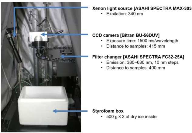
Figure 3.2.3 shows the experimental setup for measuring fluorescence images. In this experiment, the right- side fillets were used for the image measurement. Each frozen fillet sample was placed in the middle of a styrofoam box with dry ice inside to minimize temperature changes of the samples. The temperature inside the styrofoam box was kept under−50◦C. The samples were illuminated by an excitation at 340 nm, which is the most efficient excitation wavelength for freshness prediction of spotted mackerel in a frozen condition (described at 3.3.1), using MAX-303 light source (ASAHI SPECTRA). The fluorescence emitted from the sample was filtered through a band-pass filter to obtain a fluorescence image at a specific emission wavelength. The emission wavelength was controlled by changing the band-pass filter at the filter system.
The BU-56DUV CCD camera (Bitran) was used for measuring the fluorescence image at every 10 nm from 380 to 630 nm. The 2×2 binning [48] was used in the measurement with the exposure time set to 1 500 ms for each image. A total of 26 images were measured in each sample. The measured fluorescence images contained dark noise [49,50] which was corrected by subtracting a dark image acquired by closing the camera shutter and covering the lens with a lens cap so that no light could enter through the lens. The uneven distribution of illuminant was corrected by using images of a spectralon diffuse reflectance target (Labsphere) measured under the same illuminant.
Fig. 3.2.3:Experiment setup for measuring fluorescence images of the frozen fillet samples.
Camera output with excitation and emission filters
In fluorescence fingerprint imaging, the excitation wavelength and emission wavelength are controlled by attaching the band-pass filters to both the light source side (excitation) and the camera side (emission). This section describes a model that represents the camera output when using the narrow band-pass filters. The filter used in the imaging process is assumed to be an ideal band-pass filter, where the transmittance other than the wavelength to be transmitted (single wavelength) is zero. Firstly, the spectrum of illuminantI′(λex) is limited by the excitation filter and is given by:
I′(λex)=I(λex)·Fex(λex) (3.2) Fex(λex)
>0 λex=λi
=0 λex,λi
where,λexis the excitation wavelength,λiis the transmission wavelength of the excitation filter,I(λex) is the spectrum of the illuminant before transmitting the excitation filter, Fex(λex) is the transmittance of the excitation filter at λex. Then, the spectrum of the object S(λem) illumiated by I′(λex) can be described as
follows:
S(λem)=I′(λex)·{R(λex, λem)+E(λex, λem)}
(3.3) I′(λex)=
I(λex)·Fex(λex) λex=λi
0 λex,λi
R(λex, λem)=
R(λex) λex=λem
0 λex,λem
where, λem is the emission wavelength, R(λex, λem) is the reflectance rate, E(λex, λem) is the fluorescence quantum yield. The fluorescence quantum yield is the number of photons at the emission wavelength relative to the number of photons absorbed by the sample at the excitation wavelength and indicates the conver- sion efficiency between excitation light and emission light (fluorescence). Since the reflected light is much stronger than the fluorescence, λem is adjusted to be larger than λex during the measurement. Therefore, S(λem) can be transformed as follow:
S(λem)= I′(λex)·E(λex, λem) (3.4) From these equations the output of camera with the excitation and emission filters O(λex,em) is given as follows:
O(λem)=S(λem)·Fem(λem)·C(λem) (3.5) Fem(λem)
>0 λem=λ′i
=0 λem,λ′i
where,λ′i is the transmission wavelength of the emission filter,Fem(λem) is the transmittance of the emission filter, and C(λem) is the camera sensitivity. Therefore, from (3.4) and (3.5), the camera output O(λex,em) through the excitation and emission filters can be transformed as follow:
O(λex,em)=I(λex)·Fex(λex)·E(λex, λem)·Fem(λem)·C(λem) (3.6) In (3.6),E(λex, λem) represents the fluorescence properties of the sample. WhileI(λex)·Fex(λex) depends on the equipment properties on the excitation side andFem(λem)·C(λem) depends on the equipment properties on the excitation side.
Excitation and emission calibration
In order to measure the device-independence fluorescence image, excitation calibration and emission cali- bration are required. This part shows the method for excitation calibration and emission calibration.
For excitation calibration, the spectral distribution of the random illuminant with excitation filter I′ was measured using a spectralon diffuse reflectance target (Labsphere) and a spectroradiometer SR-3AR (TOP- CON). The spectral distribution obtained by the spectroradiometer can be given as (3.2). The excitation calibration function can be obtained as follows:
Nex(λex)= 1
I(λex)·Fex(λex) (3.7)
For emission calibration, the spectral distribution of the random illuminantLwas measured using a spec- tralon diffuse reflectance target (Labsphere), a spectroradiometer SR-3AR (TOPCON) and BU-56DUV CCD camera (Bitran). The spectral distribution obtained by the spectroradiometerSsd(λ) is given by (3.8). The spectral distribution obtained by the cameraSc(λem) is affected by the transmittance of the fluorescence filter Fem(λem), and the sensitivity of the cameraC(λem), resulting in (3.9).
Ssd(λem)=I(λem) (3.8)
Sc(λem)=I(λem)·Fem(λem)·C(λem) (3.9) From (3.8) and (3.9), the calibration function for the filter transmittance and camera sensitivity N(λem) can be obtained as follows:
Nem(λem)= Ssd(λem)
Sc(λem) = 1
Fem(λem)·C(λem) (3.10) In this study, the excitation side is illuminated by a single-wavelength light source with a narrow band-pass filter. Therefore, the camera outputs are only affected by the transmittance of the fluorescence filterFem(λem) and the camera sensitivityC(λem). Thus, only emission calibration was applied.
3.2.2 Experiment 2
Fish samples
In Experiment 2, two groups of spotted mackerel samples harvested from the same fish cage (Kamaishi City, Iwate Prefecture, Japan) were prepared. For the first group, normal meat was prepared using the same procedure (neck breaking) as in Experiment 1. For the second group, fish samples were killed by struggle in air for 30 min to create the burn meat. All fish samples were stored in iced water at 0◦C for 2, 4, 24, 40 h to stimulate the different freshness conditions, then filleted, vacuum packed and frozen by air blast freezer at−60◦C. There were three neck break fish samples and two struggle fish sampless for each condition. The average weight of samples was 349.7±84.9 g and the length of samples was 32.6±2.1 cm
Fluorescence image measurement
The fluorescence images of each samples were measured and calibrated with the same condition as in experi- ment 1. The samples were illuminated by an excitation at 340 nm. The fluorescence emitted from the sample was filtered through a band-pass filter to obtain a fluorescence image at every 10 nm from 380 to 630 nm.
3.3 Results and discussion
3.3.1 Experiment 1
EEM preprocessing and analysis for predicting the fish freshness
Figure 3.3.1(a) shows the EEM spectra obtained from the fish fillet measurement. The EEM was formed by recording fluorescence intensities at an emission wavelength range of 250∼800 nm under the same exci- tation wavelength range of 250∼800 nm. The raw data of EEM includes some parts that do not contain a fluorescence property. There is hypothetically no emission below the excitation based on Stokes’ shift [51].
Besides, owing to light scattering effects such as the Raman and Rayleigh effects, a typical scattering prob- lem normally exists in any excitation-emission matrix [52,53]. Scattering signals and those areas whose emission wavelengths are shorter than the excitation wavelengths do not carry relevant chemical information and should be entirely excluded from the EEM before commencing the building of the calibration models.
The preprocessed EEM spectra masked only the fluorescence area after removing those irrelevant areas is shown in Fig. 3.3.1(b).
ѣ
300 400 500 600 700 800 Em [nm]
300 400 500 600 700 800
Ex [nm]
1000 2000 3000 4000 5000 6000 7000 8000 9000
(a)
300 400 500 600 700 800 Em [nm]
300 400 500 600 700 800
Ex [nm]
500 1000 1500 2000 2500 3000 3500
(b)
Fig. 3.3.1:EEM preprocessing to remove areas that contains emission wavelengths shorter than the exci- tation wavelengths and scattering effect. (a) Raw EEM data obtained from measurement. (b) Result of EEM preprocessing.
After EEM preprocessing (i.e. removed irrelative area), the data size of each EEM was reduced to 1 054 from 3 136 variables (each variable corresponds to one excitation-emission wavelength combination of orig- inal spectra). The reduced EEM data (1 054 variables) was used to predict the measuredK-value and IMP content by a partial least squares (PLS) regression model. The PLS model was built under a leave-one-out cross-validation that used one sample as the validation and the remaining samples as the training set. The prediction accuracy is compared quantitatively using the coefficient of determination (R2), standard error of prediction (SEP) and latent variable (LV). The PLS models revealed that EEM could be used to predict K-value and IMP content with high accuracy (R2=0.86 andR2=0.84, respectively. This is very similar to the result of ElMasry et al. [15], which used all fluorescence intensity at 1 054 variables to predictK-value, with a prediction accuracy ofR2=0.86.
Selecting the most efficient excitation wavelength
In the PLS prediction models, we used all fluorescence intensity at 1 054 variables on each EEM as predictors, where each variable corresponds to one excitation-emission wavelength combination. Accordingly, when expanding this prediction model to the image, it is necessary to measure a fluorescence image at 1 054 excitation-emission wavelength combinations for each target, which mean 1 054 images. Therefore, in order to visualize the frozen fish quality expressed as K-value and IMP content more competently, reducing the high dimensionality of EEM data is required.
200 400 600 800
-0.2 0 0.2 0.4 0.6 0.8 1 (b)
R2
Excitation wavelength [nm]
200 400 600 800
-0.2 0 0.2 0.4 0.6 0.8 1 (a)
R2
Excitation wavelength [nm]
200 400 600 800
-0.2 0 0.2 0.4 0.6 0.8 1 (c)
R2
Excitation wavelength [nm]
Fig. 3.3.2:Prediction of K-value and IMP content in frozen fish at each excitation wavelength. (a), (b) Repeated PLS regression modeling using all emission wavelengths in the range under each excitation wavelength. (c) Average of (a) and (b).
In this study, the dimension of EEM was reduced by performing repeated PLS regression modeling using all emission wavelengths in the range under each excitation wavelength to identify the most effective exci- tation wavelength. The results of wavelength selection for K-value and IMP content were shown in Figs.
3.3.2(a) and 3.3.2(b), respectively and average of them in Fig. 3.3.2(c). The prediction accuracy differs for each excitation wavelength and freshness index (K-value and IMP content). In the graph of average accu- racy, at the excitation wavelength range of 300∼350 nm, the prediction of these freshness indices is lower than those of all 1 054 variables though accuracy is still high (R2is more than 0.79). The highest prediction accuracy is at an excitation wavelength of 310 nm (R2=0.83) and the next highest prediction accuracy is at an excitation wavelength of 340 nm (R2=0.80).
Due to the limitations of the equipment used in the experiment, there is no spectroradiometer that can measure whole emission wavelength (350∼570 nm) under an excitation wavelength of 310 nm. For this reason, 340 nm was chosen as the most efficient excitation wavelength instead of 310 nm to visualize fish freshness. Note that, the prediction accuracy under 340 nm is almost equivalent to 310 nm.
Emission calibration and illuminant unevenness calibration
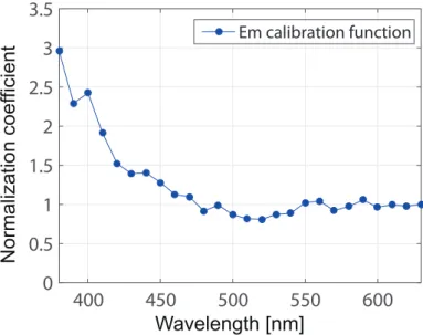
Figure 3.3.3 shows the example of illuminant unevenness calibration. Figure 3.3.4 shows the calibration function for emission filters and BU-56DUV CCD camera (Bitran), which was used for measuring fluores- cence images. In order to get the device-indepenent fluorescence images, illuminant unevenness calibration and emission calibration function was used to calibrate the fluorescence images obtained from measurement.
(b)
(a) (c)
Fig. 3.3.3:Illuminant unevenness calibration. (a) Measured fluorescence image. (b) Illuminant distribu- tion. (c) Calibrated fluorescence image.
400 450 500 550 600 0
0.5 1 1.5 2 2.5 3 3.5
Em calibration function
Wavelength [nm]
Normalization coefficient
Fig. 3.3.4:Calibration function for emission filters and BU-56DUV CCD camera (Bitran).
Visualization of the quality of frozen fish
In samples preparation (see Section 3.2.1), the fish samples were filleted after being stored in a refrigerator for a specific period, just before being vacuum packed and frozen in a freezer. Thus, in this study, we assumed that the freshness (K-value and IMP content) of the left-side fillets are the same as the freshness of the right-side fillets at the corresponding point.
In order to visualize the frozen fish freshness expressed by K-value and IMP content, we need to build a prediction model from the measured fluorescence images. The areas corresponded to the fluorescence measurement and the chemical analysis (Fig. 3.2.1) were used for analysis. For each fluorescence image, those areas were masked and the pixels value inside the mask was averaged. There were 26 fluorescence images, yielding 26 variables obtained for each point. In this study, we have 24 fish samples and two points were measured for EEM for each fish sample, consequently 26 variables at 48 points were obtained. Those 26 variables were used for predicting theK-value and IMP content at corresponding points by PLS regression model. The PLS model was built utilizing leave-one-out cross-validation which used data at one point as the validation and the remaining points as the training set. The prediction accuracy is evaluated by using the coefficient of determination (R2) and standard error of prediction (SEP).
(b)
Predicted IMP content [%]
Measured IMP content [%]
(a)
Predicted K-value [%]
Measured K-value [%]
Fig. 3.3.5:Prediction ofK-value (a) and IMP content (b) by PLS regression models using all 26 fluores- cence images.
Fig. 3.3.5 shows the result of predictingK-value and IMP content (measured in the left-side fillets) at EEM measurement points (Fig. 3.2.1) by using fluorescence images. The prediction accuracy of the PLS models from the measured fluorescence images wereR2=0.78 forK-value andR2=0.82 for IMP content. These are lower than those prediction models using all 1 054 variables of EEM (R2=0.86 forK-value andR2=0.84 for IMP content). However, the aim of the visualization is to make visible the spatial-temporal freshness changes of a whole sample with acceptable accuracy. Thus, the prediction accuracy of these PLS models (R2=0.78 forK-value andR2=0.82 for IMP content) is high enough and are acceptable for the visualization.
From the obtained prediction models, the distributions of K-value and IMP content can be estimated by combining the parameters of the prediction models with fluorescence image at corresponding emission wavelength to obtain the freshness distribution image as follows:
yn=β380xn380+β390xn390+· · ·+β630xn630+β0 (3.11)
wheren is the sample number,β is the parameters of the prediction model,x is the fluorescence image of sample nat specific emission wavelength measured at Section 3.2.1. The result of the visualization of the distributions ofK-value and IMP content are shown in Fig. 3.3.6 and Fig. 3.3.7. There were three samples for each storage time condition. The samples in Fig. 3.3.6 are same as samples in Fig. 3.3.7, which are result
of visualizeK-value and IMP content, respectively. As a result,K-value increased in accordance with ice storage time. On the other hand, IMP content rapidly increased for the storage period from 0 to 1 day, and then gradually decreased from 2 to 9 days.
Fig. 3.3.6:Visualization of the spatial-temporal changes ofK-value in frozen fish fillets.
Fig. 3.3.7:Visualization of the spatial-temporal changes of IMP content in frozen fish fillets.
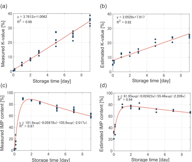
The measuredK-value and IMP content obtained from chemical analysis are shown in Figs. 3.3.8(a) and Fig. 3.3.8(c), respectively. As a result, K-value increased linearly with storage time. On the other hand, IMP content increased dramatically from 0 % to 90 % for the samples from 0 to 1 day, and then gradually decreased for the samples from 2 to 9 days. From the visualization result obtained in Fig. 3.3.6 and Fig.
3.3.7, the average of estimatedK-value and IMP content in each of the fish samples were calculated. The estimated K-value and IMP content are shown in Figs. 3.3.8(b) and 3.3.8(d), respectively. As expected, the changes ofK-value and IMP content obtained from chemical analysis and estimated from fluorescence images showed the same trend and as same as the previous studies [43,54,55], ATP inside the muscle is decomposed rapidly. After the decomposition of ATP, ADP and AMP are also decomposed quickly and advance to IMP in a stroke, occur instantaneous accumulation of IMP. Furthermore, IMP thus formed is slowly converted to HxR and then to Hx, which means the slowly increasing ofK-value. The comparison of measured and estimatedK-value and IMP content obtained from chemical analysis at three parts (back, belly, tail) are shown in Fig. 3.3.9. The change in bothK-value and IMP content differ for each part of the fish.
The back part and tail part, which were used for chemical analysis, showed the highestK-value compared to other parts. Therefore, the average of estimatedK-value and IMP content change is slightly smoother than the measured value, which was point measurement.
This result suggested that the purposed method could accurately visualize the distribution of bothK-value and IMP content using only one excitation light and be practical for large-scale commercial purposes with a vast number of fish or large fish such as tuna.
(a)
Storage time [day]
Measured K-value [%]
(d)
Estimated IMP content [%]
Storage time [day]
(b)
Measured IMP content [%]
Storage time [day]
(c)
Estimated K-value [%]
Storage time [day]
Fig. 3.3.8:Comparison of measured and estimated values of K-values and IMP content. (a) (c) The mea- suredK-value, IMP content obtained from chemical analysis. (b) (d) The estimatedK-value, IMP content calculated by averaging the distribution images obtained in Fig. 3.3.6 and Fig.
3.3.7, respectively.
0 2 4 6 Storage time [day]
0 20 40 60 80 100
Predicted IMP value [%]
Back part Belly part Tail part
8
0 2 4 6
Storage time [day]
0 10 20 30 40
Predicted K-value [%]
Back part Belly part Tail part
8
(a) (b)
(c) (d)
Fig. 3.3.9:Comparison of measured and estimated K-values and IMP content at different parts. (a) (c) The measured K-value, IMP content at three parts (back, belly, tail) obtained from chemical analysis. (b) (d) The estimatedK-value, IMP content at three parts (back, belly, tail) calculated by averaging the distribution images obtained in Fig. 3.3.6 and Fig. 3.3.7, respectively.