China's provincial carbon emission transfers and the effectiveness of mitigation polices

China's provincial carbon emission transfers and the effectiveness of mitigation polices

著者 Gao Yuning, Li Meng, Bo Meng, Xue Jinjun

権利 (C)2020 by Institute of Developing Economies, JETRO and the Institute of Contemporary China Studies,  Tsinghua University. No part of this publication may be reproduced without the

prior permission of the  IDE‑JETRO and the Institute of Contemporary China Studies, Tsinghua University.

journal or

publication title

IDE Discussion Paper

volume 775

year 2020‑03

URL http://hdl.handle.net/2344/00051685

INSTITUTE OF DEVELOPING ECONOMIES

IDE Discussion Papers are preliminary materials circulated to stimulate discussions and critical comments

Keywords:

Input-Output Analysis; Chinese economy

JEL classification:

IDE DISCUSSION PAPER No. 775

China’s Provincial Carbon Emission Transfers and the Effectiveness of Mitigation Polices

Yuning GAO¹, Meng LI¹, Bo MENG^2*, Jinjun XUE

March 2020

Abstract

The complexity of shared emissions responsibility for carbon transfers in various regions of China has further raised additional challenges for energy savings and carbon mitigation efforts.

This paper establishes an extended provincial input-output (IO) model for each province to calculate carbon emissions based on production, consumption, and transfers from 2005 through 2015, and examines whether carbon mitigation policies can effectively promote energy conservation and emissions reduction in the various provinces. The empirical analysis established that: (1) an increase in the implementation strength of mitigation policy can effectively reduce production-based carbon emissions amongst the different provinces; (2) stricter mitigation policy increases the possibility that a province will transfer more of their emissions to other areas, thus causing a net emissions outflow; and (3) subsequent policy enforcement will weaken once mitigation goals are accomplished. Therefore, this paper repudiates the accepted belief that mitigation policy effectively controls carbon emissions, especially for production-based emissions. More refined policy design and supplementation is needed when considering consumption-based emissions and related carbon transfers.

The Institute of Developing Economies (IDE) is a semigovernmental, nonpartisan, nonprofit research institute, founded in 1958. The Institute merged with the Japan External Trade Organization (JETRO) on July 1, 1998.

The Institute conducts basic and comprehensive studies on economic and related affairs in all developing countries and regions, including Asia, the Middle East, Africa, Latin America, Oceania, and Eastern Europe.

The views expressed in this publication are those of the author(s). Publication does not imply endorsement by the Institute of Developing Economies of any of the views expressed within.

INSTITUTE OF DEVELOPING ECONOMIES (IDE), JETRO 3-2-2, WAKABA,MIHAMA-KU,CHIBA-SHI

CHIBA 261-8545, JAPAN

©2020 by Institute of Developing Economies, JETRO and the Institute of Contemporary China Studies, Tsinghua University. No part of this publication may be reproduced without the prior permission of the IDE-JETRO and the Institute of Contemporary China Studies, Tsinghua University.

1

China’s Provincial Carbon Emission Transfers and the Effectiveness of Mitigation Polices

Yuning GAO¹, Meng LI¹, Bo MENG², Jinjun XUE³ Abstract

The complexity of shared emissions responsibility for carbon transfers in various regions of China has further raised additional challenges for energy savings and carbon mitigation efforts. This paper establishes an extended provincial input-output (IO) model for each province to calculate carbon emissions based on production, consumption, and transfers from 2005 through 2015, and examines whether carbon mitigation policies can effectively promote energy conservation and emissions reduction in the various provinces. The empirical analysis established that: (1) an increase in the implementation strength of mitigation policy can effectively reduce production- based carbon emissions amongst the different provinces; (2) stricter mitigation policy increases the possibility that a province will transfer more of their emissions to other areas, thus causing a net emissions outflow; and (3) subsequent policy enforcement will weaken once mitigation goals are accomplished. Therefore, this paper repudiates the accepted belief that mitigation policy effectively controls carbon emissions, especially for production-based emissions. More refined policy design and supplementation is needed when considering consumption-based emissions and related carbon transfers.

Keywords: Carbon Emission; Carbon Transfer; Mandatory Mitigation Target; Input-Output Analysis; Chinese economy

JEL Classification: Q54, Q58, C67, C54

1: School of Public Policy and Management, Tsinghua University, China 2: Institute of Developing Economies – JETRO, Japan ([email protected]) 3: School of Economics, Nagoya University, Japan

Acknowledgements: We thank Prof. Kyoji FUKAO (IDE-JETRO), Mr. Makoto ABE (IDE-JETRO) for their helpful comments, Ms. Maiko KUBOTA (IDE-JETRO) for her kind administrative support. This paper is partly supported IDE/JETRO-Institute of Contemporary China Studies (Tsinghua University) international joint works (2019-2020), and Japan’s Grants-in-Aid for Scientific Research (KAKEN)

“China’s Belt and Road Initiative and its Impact on the Earth Environment” (#18K01608).

2

Table of Contents

1. INTRODUCTION ... 3

2. LITERATURE REVIEW ... 4

3. METHODS FOR CARBON EMISSIONS ACCOUNTING ... 5

Figure 1. Accounting Framework for Carbon Emissions. ... 6

Table 2. The Carbon Emissions Transfer Matrix, Under an Extended Provincial IO Table. ... 8

4. DATA SOURCES AND THE RESULTS OF ACCOUNTING... 9

Figure 2. Distribution of Carbon Emissions and Transfers in the Provinces. ... 10

5. EMPIRICAL ANALYSIS AND RESULTS ... 11

5.1CONSTRUCTION OF POLICY VARIABLES ... 11

Table 3. Statistical Descriptions of Major Policy Variables. ... 12

5.2THE EMISSION REDUCTION EFFECT OF MANDATORY MITIGATION POLICIES ... 12

Table 4. Emission Reduction Effect of Mandatory Mitigation Policies. ... 13

5.3THE IMPACT OF MITIGATION POLICIES ON EMISSIONS TRANSFERS ... 14

Table 5. Impact on Net Emissions Transfers. ... 14

6. THE EFFECTIVENESS OF IMPLEMENTATION INTENSITY OF MITIGATION TARGETS ... 15

Table 6. The Effectiveness of Mitigation Policy after the Achievement of FYP Targets. ... 15

Figure 3. Implementation Intensity of Mitigation Policies, 2005 to 2015. ... 17

7. CONCLUSIONS AND POLICY IMPLICATIONS ... 18

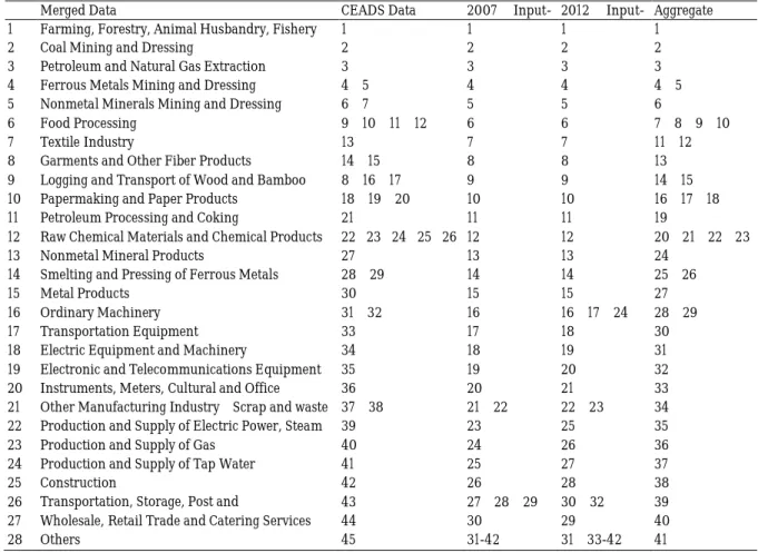
APPENDIX A. CONCORDANCE OF INDUSTRIES ... 23

Table A1. Concordance of Industries from Different Data. ... 23

APPENDIX B. PROVINCES4 \H NDUSTRIES FROM DIFFERENT DATA.S, 2005 T23 Figure B1. Provinces55 \h ndustries from Different Data.s, 2005 to 2015. FYP Ta24 Figure B2. Net Carbon Transfers and Carbon Intensity, 2005 to 2015. ... 24

Figure B3. Net Carbon Transfer: Amount and Structure of Beijing. ... 25

Figure B4. Net Carbon Transfer: Amount and Structure of Hebei. ... 25

3 1. Introduction

As of 2005, China surpassed the United States (US) as the world’s largest carbon emitter and its annual carbon emissions have been growing rapidly along with its economic development ever since (Minx, 2011). Its emissions declined for the first time in 2014 but quickly rebounded thereafter. China faces arduous mitigation challenges (Lin & Liu, 2010) and is making tangible efforts. In 2009 at the Copenhagen Conference, China announced the goal of reducing 40-45% of its carbon dioxide (CO2) emissions per unit of gross domestic product (GDP) by 2020. In the US- China Joint Announcement on Climate Change in 2014, China also claimed to expect an emissions peak in the year 2030, when non-fossil fuel energy would comprise 20% of all energy consumption.

China further set its goal for reducing CO2 emissions by 60% to 65%—lower than that of 2005—

per unit of GDP by 2030. It is important to note that with global economic integration, a considerable amount of China’s carbon emissions is generated by the consumers at the end of the global value chain (GVC) of China’s exports (Meng et al., 2018). A similar phenomenon also occurs in China’s domestic value chain, which is composed of its various provinces. Therefore, current mitigation policies need to clarify emissions responsibility first, both on the international and domestic levels.

On the other hand, China has formulated corresponding mitigation policies based on administrative and market means. The Five-Year Program (FYP) policy is an important administrative tool for management of China’s energy conservation and emissions reduction.

Contents related to those subjects in FYPs have been increasing continuously in terms of quantity and policy details (Yuan & Zuo, 2011). According to the FYPs, China’s energy policy can be divided into two stages. The first phase is to expand energy production and consumption increase rapidly.

From the first to the tenth FYP, there were clear goals for coal production. Targets of total energy production existed from the sixth to the ninth FYP. The tenth FYP become a turning point for not setting such targets anymore, indicating that the government will no longer simply encourage the expansion of energy production. The second phase starts from the eleventh FYP until now. During this period, targets for energy conservation and emissions reductions have increased in quantity as well as quality. In the eleventh FYP, China proposed mandatory targets to reduce 10% of its total pollutant emissions and 20% of its energy consumption per unit GDP. It decomposed these targets into governments and enterprises at all levels and set energy-savings targets under the “One Thousand Enterprises Energy Saving and Emission Reduction Action Plan.” Completion of those targets has been incorporated into performance appraisals of governments and state-owned enterprises (SOEs) (State Council, 2011). On carbon emissions, the eleventh FYP proposed a general and broad mitigation target, addressed as “effectively controlling greenhouse gas (GHG) emissions” (State Council, 2006). In the twelfth FYP, however, China proposes a 16% reduction in energy consumption and a 17% reduction in CO2 emissions per unit of GDP. It would reduce 8%

of total COD and 10% of ammonia nitrogen and nitrogen oxide emissions, respectively. China also plans to level its forest coverage up to 21.66% and increase 600 million cubic meters of forest stock.

In January 2012, Plans for GHG Emission Control in the twelfth FYP was issued (State Council, 2011). Apparently, the twelfth FYP has more detailed targets for carbon emissions. It has a chapter focusing solely on carbon emissions and climate change issues. This chapter lays out many mitigation measures to ease energy consumption intensity and carbon intensity, such as adjusting industrial and energy structures, promoting energy conservation and efficiency, and increasing forest carbon absorption. From the eleventh FYP to the twelfth FYP, the numbers of indices related

4

to resources and the environment increase from eight to 12. Mandatory indices increase to 11 from six, suggesting that the government is making a stronger effort with mitigation policies.

According to calculations of carbon emissions based on production, consumption, and net carbon transfers of China’s provinces between 2005 and 2015, this paper clarifies the direct and indirect carbon emissions responsibilities of each province. By including policy variables into an empirical analysis framework, this paper tries to answer the following questions: Do these policies effectively promote mitigation? What kind and which part of mitigation are promoted? Do policies promote or undermine carbon balances in provinces that have different characteristics? Do the FYP’s mitigation policies have a sustainable impact?

This paper is organized as follows. Section 2 reviews the relevant literature on extended input- output analysis and policy impact on energy conservation and emissions reduction. Section 3 establishes and describes various methods for carbon emissions accounting, and expands the traditional method to include an extended provincial input-output model to calculate carbon emissions based on production, consumption, and other criteria. Section 4 outlines data sources, provides the results of emissions accounting calculations, and builds a carbon emissions database for 30 provinces for the years between 2005 and 2015. Sections 5 and 6 carry out empirical calculations and present results; Section 5 analyzes the impact of mitigation policies of different emissions calibers and components and Section 6 examines the implementation stringency of mitigation policies in the remaining years after the realization of mitigation targets. Section 7 provides concluding remarks and discusses policy implications.

2. Literature Review

Due to its importance, a large number of scholars have conducted many research studies on the subject of carbon emissions estimation, inter-regional carbon transfer and spillover effects, and the policy impacts on drivers of growing emissions. This paper is concerned with two elements of that research, including the measurement of “real” carbon emissions and the factors driving emissions based on those calculations.

The literature on measuring “real” carbon emissions primarily consists of the production- based and consumption-based approaches, namely, “give credit where credit is due” (Koopman, 2010). Calculations of carbon emissions have two major principles, producer-based and consumer- based (Atkinson et al., 2011; Peters, 2008; Steininger et al., 2014). The producer-based principle allocates emissions to producers. The carbon emissions from the production of all goods and services in a certain region are used to either meet consumption demands locally or are exported elsewhere. The consumer-based principle, on the other hand, attributes emissions to the final consumer. Emissions of the goods and services consumed by local residents, businesses, and governments in a certain region are either directly generated from the local market or are purchased from other regions (Davis and Caldeira, 2010; Feng et al., 2014; Takahashi et al., 2014;

Tian et al., 2014; Wang et al., 2018; Wiedmann et al., 2011). To clarify the emissions responsibilities of producers and consumers (Guan et al., 2014; Lenzen et al., 2007), the accurate calculation of consumption-based emissions must trace the carbon emissions embedded in inter- regional trade (Jakob et al., 2014; Peters and Hertwich, 2008a, 2008b; Steininger et al., 2014).

Scholars first apply input-output analysis (IOA) to environmental areas (Hertwich et al., 2009;

Leontief, 1970; Su et al., 2010; Su and Ang, 2014; Wiedmann et al., 2007; Wiedmann, 2009), and confirm the accuracy and superiority of the multi-regional input-output model (MRIO) (Liu et al.,

5

2017). They then began using the MRIO for the calculation of international carbon transfers (Liu and Fan, 2017; Meng et al., 2018) and inter-regional emissions levels within nations. On such a basis, scholars used the extended input-output model (EIO) to calculate China’s “real” carbon emissions and discuss carbon transfers within China. Some research examined China’s inter- regional carbon spills in 2002, 2007, and 2012. They estimated the consumption-based carbon emissions inventory on the basis of production-based emissions (Wang et al., 2016; Zhao et al., 2015). Some scholars believed that the carbon spillovers and transfers embedded in inter-regional trade were very common in China due to the domestic disparity between the economy and technology (Duan et al., 2018; Feng et al., 2012; Feng et al., 2013; Meng et al., 2013; Liang et al., 2007; Liu et al., 2015; Zhang et al., 2018a). Some studies embedded China’s inter-regional input- output table into the global table in order to analyze China’s inter-regional carbon transfers from the perspective of their participation in GVCs (Guo et al., 2012; Pei et al., 2018; Yu, 2014; Zhang et al., 2018b).

The literature on driving factors mainly conducts studies through empirical analysis, such as regression analyses based on models such as the IPAT, STRIPAT, and Kaya (Dietz and Rosa, 1994;

Ehrlich and Holdren, 1971, 1972; Yoichi Kaya, 1989), as well as structural decomposition analysis.

Recent literature focuses on the impact of mitigation policy on carbon emissions and economic development, in particular, the FYPs (Tang et al., 2016; Yuan and Zuo, 2011), carbon trade (Cong and Wei, 2010; Li et al., 2018; Dai et al., 2018), and energy or carbon taxes (Chen and Guo, 2017;

Fan et al., 2018; Zheng et al., 2016; Zou et al., 2018). They further divided emission responsibilities for each province in China (Wang et al., 2018), proposed policy recommendations (Lin and Liu, 2010), and concluded that China should alter its energy structure and promote energy conservation to achieve mitigation targets.

In summary, with the support of a larger database and expanded IOA methods, the existing literature re-calculated production- and consumption-based carbon emissions at the international and domestic levels, respectively. They also evaluated or simulated the impacts of various types of policies. However, most conducted research at a larger regional level rather than at a provincial level, for a given year, or created case studies of specific provinces. This paper extends the current MRIO model to establish provincial-level panel data for production-based, consumption-based, and transferred emissions. This method has several advantages. Firstly, it can trace the “real”

carbon emissions for different industries and individual provinces by expanding the existing MRIO.

In addition, this paper offers a more consistent and continuous time span that covers several FYPs and makes evaluations more systematic. Moreover, this paper establishes better research reliability by taking each province’s economy, population, natural resources, and policy differences into consideration when conducting empirical analyses at the provincial level.

3. Methods for Carbon Emissions Accounting

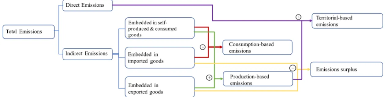
There are two causes of carbon emissions. Carbon can be emitted from the direct combustion of fuels, such as cooking and heating, which is referred to as direct emissions. The other cause is consumption-based. Although no direct emissions are created during consumption, products consumed by residents, businesses, and governments cause emissions during their production process. This type is called indirect emissions.

Therefore, under a complete carbon calculation framework, carbon emissions consist of two major components, direct and indirect emissions. Indirect emissions contain three distinct

6

branches: emissions that are embedded in products that are produced and consumed locally, those that are embedded in imported products, and those that exist in exported products. Based on different calculation principles, these three components can add up to a variety of results.

Combining carbon emissions embedded in local production and consumption with emissions embedded in import transfers yields the total for consumption-based emissions. One can calculate production-based emissions by adding the emissions embedded in local production to those in export transfers. One can also calculate net carbon imports, namely, the carbon surplus, by subtracting the emissions embedded in export transfers from those in import transfers.

Furthermore, we are able to obtain carbon emissions based on the regional geographical boundaries by adding direct emissions and production-based emissions together. The framework for carbon emissions calculations is shown in Figure 1.

Figure 1. Accounting Framework for Carbon Emissions.

The most widely used method for carbon emissions calculations is the MRIO. Researchers calculate China’s inter-regional carbon transfers based on this model (Feng et al., 2013; Liu et al., 2015; Wang et al., 2017). The MRIO shows its superiority by accurately include flows of carbon emission in different industries and regions (Liu et al., 2017). Since the inter-regional input-output table of China is only available for the years of 2007 and 2012, and it is aggregated at the regional or industry level, the MRIO is more suitable for reflecting carbon transfers and responsibility commitments amongst major regions, rather than calculating provincial indirect emissions.

In calculations, direct emissions can be measured by energy consumptions. Indirect emissions, by expanding the MRIO into an environmentally EIO, can be calculated by tracing all final consumption back to its production. The EIO serves as a bridge that connects final consumption to carbon emissions. Through the “Final Use-Total Output-Carbon Emissions”

process, the EIO tracks all indirect emissions. On the other hand, the EIO also connects consumption-based emissions at the input end to production-based emissions at the output end.

It unifies two emissions calculation calibers into one unified model.

Therefore, this study expands the IOA to an extended provincial IO model, which is a derivative of, or an exception to, the MRIO. An extended provincial input-output (IO) table distinguishes between “local” and the “rest of China” for each province. This table enables accurate emissions calculations across all provinces for consecutive years. Instead of emphasizing the detailed distribution of carbon transfers between regions, it focuses on the measurement of total production-based and consumption-based emissions in different industries across various provinces in different years. For a given province i, the extended provincial IO table can be obtained by combining the regional and national IO tables, as shown in Table 1.

7

Table 1. Structure of the Extended Provincial IO Table.

The extended provincial IO model still satisfies the basic equation:

𝑋𝑋= (𝐼𝐼 − 𝐴𝐴^∗)⁻¹𝑌𝑌^∗ (1) 𝐶𝐶^∗=𝐹𝐹^∗(𝐼𝐼 − 𝐴𝐴^∗)⁻¹𝑌𝑌^∗ (2)

𝐶𝐶^𝑀𝑀=𝐹𝐹�𝐼𝐼 − 𝐴𝐴�⁻¹𝑌𝑌^𝑀𝑀 (3)

𝑌𝑌=𝑌𝑌^∗+𝑌𝑌^𝑀𝑀 (4)

𝐶𝐶=𝐶𝐶^∗+𝐶𝐶^𝑀𝑀 (5)

In which:

𝑋𝑋: Total Output for Province 𝑖𝑖

𝐴𝐴^∗, 𝐴𝐴: Direct consumption coefficient matrix for Province 𝑖𝑖 and the Rest of China (𝐼𝐼 − 𝐴𝐴^∗)⁻¹, �𝐼𝐼 − 𝐴𝐴�⁻¹: Leontief Inverse Matrix for Province 𝑖𝑖 and the Rest of China

Y, 𝑌𝑌^∗, 𝑌𝑌^𝑀𝑀: Sum of Final Use, Final Use from Province 𝑖𝑖, Final Use Imported from the Rest of China and foreign countries

𝐹𝐹^∗, 𝐹𝐹: Carbon emission coefficient for Province 𝑖𝑖 and the Rest of China

C, 𝐶𝐶^∗, 𝐶𝐶^𝑀𝑀: Carbon emissions caused by final use of Province 𝑖𝑖, that produced in Province 𝑖𝑖, produced in the Rest of China,

We continue to sub-divide the final use of local products and the final use of imported products. According to their specific flows, we can sub-divide these into five sectors: urban consumption, rural consumption, government consumption, capital formation, and exports.

𝑌𝑌^∗=𝑌𝑌_𝑈𝑈^{𝐶𝐶𝐶𝐶𝐶𝐶∗}+𝑌𝑌_𝑅𝑅^{𝐶𝐶𝐶𝐶𝐶𝐶∗}+𝑌𝑌_𝐺𝐺^{𝐶𝐶𝐶𝐶𝐶𝐶∗}+𝑌𝑌^{𝐶𝐶𝐶𝐶𝐶𝐶∗}+𝐸𝐸^∗ (6)

𝑌𝑌^𝑀𝑀=𝑌𝑌_𝑈𝑈^{𝐶𝐶𝐶𝐶𝐶𝐶_𝑀𝑀}+𝑌𝑌_𝑅𝑅^{𝐶𝐶𝐶𝐶𝐶𝐶_𝑀𝑀}+𝑌𝑌_𝐺𝐺^{𝐶𝐶𝐶𝐶𝐶𝐶_𝑀𝑀}+𝑌𝑌^{𝐶𝐶𝐶𝐶𝐶𝐶_𝑀𝑀}+𝐸𝐸^𝑀𝑀 (7) We expand 𝑌𝑌^∗ and 𝑌𝑌^𝑀𝑀0F1:

𝐶𝐶^∗ =𝐹𝐹^∗(𝐼𝐼 − 𝐴𝐴^∗)⁻¹(𝑌𝑌_𝑈𝑈^{𝐶𝐶𝐶𝐶𝐶𝐶∗}+𝑌𝑌_𝑅𝑅^{𝐶𝐶𝐶𝐶𝐶𝐶∗}+𝑌𝑌_𝐺𝐺^{𝐶𝐶𝐶𝐶𝐶𝐶∗}+𝑌𝑌^{𝐶𝐶𝐶𝐶𝐶𝐶∗}+𝐸𝐸^∗)

=𝐶𝐶_𝑈𝑈^{𝐶𝐶𝐶𝐶𝐶𝐶∗}+𝐶𝐶_𝑅𝑅^{𝐶𝐶𝐶𝐶𝐶𝐶∗}+𝐶𝐶_𝐺𝐺^{𝐶𝐶𝐶𝐶𝐶𝐶∗}+𝐶𝐶^{𝐶𝐶𝐶𝐶𝐶𝐶∗}+𝐶𝐶^𝐸𝐸 (8)

𝐶𝐶^𝑀𝑀=𝐹𝐹�𝐼𝐼 − 𝐴𝐴�⁻¹�𝑌𝑌_𝑈𝑈^{𝐶𝐶𝐶𝐶𝐶𝐶𝑀𝑀}+𝑌𝑌_𝑅𝑅^{𝐶𝐶𝐶𝐶𝐶𝐶𝑀𝑀}+𝑌𝑌_𝐺𝐺^{𝐶𝐶𝐶𝐶𝐶𝐶𝑀𝑀}+𝑌𝑌^{𝐶𝐶𝐶𝐶𝐶𝐶𝑀𝑀}�

=𝐶𝐶_𝑈𝑈^{𝐶𝐶𝐶𝐶𝐶𝐶𝑀𝑀}+𝐶𝐶_𝑅𝑅^{𝐶𝐶𝐶𝐶𝐶𝐶𝑀𝑀}+𝐶𝐶_𝐺𝐺^{𝐶𝐶𝐶𝐶𝐶𝐶𝑀𝑀}+𝐶𝐶^{𝐶𝐶𝐶𝐶𝐶𝐶𝑀𝑀} (9)

1 𝐸𝐸^{𝐼𝐼𝑀𝑀} refers tore-export Trade which is not consumed. It should be excluded when calculating total carbon emissions.

8 Therefore, we can calculate total carbon emissions C:

𝐶𝐶=𝐶𝐶^∗+𝐶𝐶^𝑀𝑀

= (𝐶𝐶_𝑈𝑈^{𝐶𝐶𝐶𝐶𝐶𝐶∗}+𝐶𝐶_𝑅𝑅^{𝐶𝐶𝐶𝐶𝐶𝐶∗}+𝐶𝐶_𝐺𝐺^{𝐶𝐶𝐶𝐶𝐶𝐶∗}+𝐶𝐶^{𝐶𝐶𝐶𝐶𝐶𝐶∗}+𝐶𝐶^𝐸𝐸) +�𝐶𝐶_𝑈𝑈^{𝐶𝐶𝐶𝐶𝐶𝐶𝑀𝑀}+𝐶𝐶_𝑅𝑅^{𝐶𝐶𝐶𝐶𝐶𝐶𝑀𝑀}+𝐶𝐶_𝐺𝐺^{𝐶𝐶𝐶𝐶𝐶𝐶𝑀𝑀}+𝐶𝐶^{𝐶𝐶𝐶𝐶𝐶𝐶𝑀𝑀}�

= (𝐶𝐶_𝑈𝑈^{𝐶𝐶𝐶𝐶𝐶𝐶∗}+𝐶𝐶_𝑈𝑈^{𝐶𝐶𝐶𝐶𝐶𝐶𝑀𝑀}) + (𝐶𝐶_𝑅𝑅^{𝐶𝐶𝐶𝐶𝐶𝐶∗}+𝐶𝐶_𝑅𝑅^{𝐶𝐶𝐶𝐶𝐶𝐶𝑀𝑀}) + (𝐶𝐶_𝐺𝐺^{𝐶𝐶𝐶𝐶𝐶𝐶∗}+𝐶𝐶_𝐺𝐺^{𝐶𝐶𝐶𝐶𝐶𝐶𝑀𝑀}) + (𝐶𝐶^{𝐶𝐶𝐶𝐶𝐶𝐶∗}+𝐶𝐶^{𝐶𝐶𝐶𝐶𝐶𝐶𝑀𝑀}) +𝐶𝐶^𝐸𝐸

=𝐶𝐶_𝑈𝑈^{𝐶𝐶𝐶𝐶𝐶𝐶}+𝐶𝐶_𝑅𝑅^{𝐶𝐶𝐶𝐶𝐶𝐶}+𝐶𝐶_𝐺𝐺^{𝐶𝐶𝐶𝐶𝐶𝐶}+𝐶𝐶^{𝐶𝐶𝐶𝐶𝐶𝐶}+𝐶𝐶^𝐸𝐸 (10)

Similarly, we can also aggregate those sub-divided carbon emissions categories to obtain total emissions for household consumption, total emissions from household and government, and emissions generated by local products and services that include consumption and fixed capital.² These three categories are listed below.

𝐶𝐶^𝐻𝐻=𝐶𝐶_𝑈𝑈^{𝐶𝐶𝐶𝐶𝐶𝐶}+𝐶𝐶_𝑅𝑅^{𝐶𝐶𝐶𝐶𝐶𝐶} (11)

𝐶𝐶^{𝐶𝐶𝐶𝐶𝐶𝐶}=𝐶𝐶^𝐻𝐻+𝐶𝐶_𝐺𝐺^{𝐶𝐶𝐶𝐶𝐶𝐶} (12)

𝐶𝐶𝐶𝐶𝐶𝐶𝐶𝐶&𝐶𝐶𝐶𝐶𝐶𝐶=𝐶𝐶^{𝐶𝐶𝐶𝐶𝐶𝐶}+𝐶𝐶^{𝐶𝐶𝐶𝐶𝐶𝐶} (13)

Net carbon transfers can be shown as follows.

𝐶𝐶^𝐵𝐵=𝐶𝐶^𝑀𝑀− 𝐶𝐶^𝐸𝐸 (14)

Production-based carbon emissions, consumption-based emissions, and their relationship, are shown as follows.

𝐶𝐶^𝐶𝐶 =𝐶𝐶^{𝐶𝐶𝐶𝐶𝐶𝐶}+𝐶𝐶^{𝐶𝐶𝐶𝐶𝐶𝐶}+𝐶𝐶^𝐸𝐸 (15)

𝐶𝐶^𝐶𝐶 =𝐶𝐶^{𝐶𝐶𝐶𝐶𝐶𝐶}+𝐶𝐶^{𝐶𝐶𝐶𝐶𝐶𝐶}+𝐶𝐶^𝑀𝑀 (16)

𝐶𝐶^𝐶𝐶 = (𝐶𝐶^{𝐶𝐶𝐶𝐶𝐶𝐶}+𝐶𝐶^{𝐶𝐶𝐶𝐶𝐶𝐶}+𝐶𝐶^𝐸𝐸) + (𝐶𝐶^𝑀𝑀− 𝐶𝐶^𝐸𝐸) =𝐶𝐶^𝐶𝐶+𝐶𝐶^𝐵𝐵 (17)

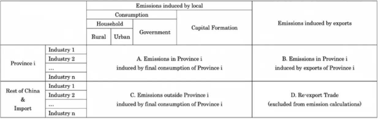
The Carbon Emissions Matrix, measured by the extended provincial IO table, can be seen in Table 2.

Table 2. The Carbon Emissions Transfer Matrix, Under an Extended Provincial IO Table.

From Table 2, we can now calculate production-based carbon emissions, consumption-based carbon emissions, and transferred emissions, respectively. We arrive at the production-based carbon emissions of province 𝑖𝑖 by adding A, carbon emissions in province 𝑖𝑖 caused by final consumption in province 𝑖𝑖, with B, carbon emissions in province 𝑖𝑖 caused by exports of province 𝑖𝑖, horizontally. This yields consumption-based carbon emissions by combining A, carbon emissions in province 𝑖𝑖 caused by final consumption of province 𝑖𝑖 with C, carbon emissions for the 𝑅𝑅𝑅𝑅𝑅𝑅𝑅𝑅 𝑜𝑜𝑜𝑜 𝐶𝐶ℎ𝑖𝑖𝑖𝑖𝑖𝑖 that are caused by final consumption in province 𝑖𝑖, vertically. Furthermore, we can measure the net carbon transfer (carbon surplus) of province 𝑖𝑖 by subtracting B, carbon

2 Carbon emissions used by local goods and services that are consumed locally equal the sum of household consumption, government consumption, and capital formation. Corresponding to the local end in final use, it can be sub-divided into rural consumption, urban consumption, government consumption, and capital formation.

9

emissions in province 𝑖𝑖 caused by exports of province 𝑖𝑖 from C, carbon emissions in the 𝑅𝑅𝑅𝑅𝑅𝑅𝑅𝑅 𝑜𝑜𝑜𝑜 𝐶𝐶ℎ𝑖𝑖𝑖𝑖𝑖𝑖 caused by final consumption in province 𝑖𝑖.

The extended provincial IO model has three major advantages. The first is that the IO data comes directly from the National Bureau of Statistics with less artificial processing and estimation.

The data source is more authoritative, accurate, and easier to access. Secondly, as a transformation of the MRIO, it retains the accuracy of the MRIO. Moreover, it enables us to measure carbon emissions for each individual province and provides provincial penal data that is feasible for use in further empirical analysis.

4. Data Sources and the Results of Accounting

The extended provincial IO model requires three categories of data, which are carbon intensity, Leontief inverse matrix, and final consumption.

Constructing carbon intensity data includes two steps. One is the collection of carbon emissions from various industries across different regions. The other is to collect the total output for each region and industry. Industry-level emissions data in this paper is from the CEADS database (Shan et al., 2017), which covers direct emissions from 45 industries, urban and rural households, 47 sections in total. The total output data in this paper is directly from the regional input-output table in certain feasible years. In other years, data of 36 industrial sectors, except for architecture, is from China Industry Economy Statistical Yearbook, China Industry Statistical Yearbook, or China Economic Census Yearbook. Data on agriculture, forestry, animal husbandry, fishery, and architecture come from the National Bureau of Statistics website. Data of service industry is calculated based on added value and its growth rate.

The Leontief inverse matrix comes from the national and provincial level IO tables released by the National Bureau of Statistics for the years 2007 and 2012 (NBS, 2011; NBS, 2016), covering 42 departments in 30 provinces, with the exception of Tibet. In this paper, we first calculate the direct input coefficient matrix through the intermediate input matrix and total output. On that basis, we obtain the Leontief inverse matrix.

Data regarding final use is derived from sub-divisions of the National Bureau of Statistics’

provincial-level gross regional products (by expenditure approach) for the years of 2005 through 2016. It consists of rural consumption, urban consumption, capital formation, and the net outflow of goods and services. This paper, combines the structure of final use for each province in the IO table, and then splits the total for final use of each type to obtain the data for final use in each year, province, and industry.

This paper combines the IO tables, CEADS emissions data, and total output data for different years in 28 business sectors, including general agriculture, forestry, animal husbandry, and fisheries, 24 industries, and three service sectors. Appendix A shows these specific correspondences.

Based on the models above, this paper uses the direct consumption coefficient matrix and carbon emissions coefficient matrix for each province to estimate the local carbon emissions embedded in self-consumed and outflowed products. It uses the direct consumption coefficient matrix and carbon emissions coefficient matrix in ROC to estimate carbon emissions in ROC that are embedded in imported goods and services to the local market. The panel database for carbon emissions in 30 provinces between 2005 and 2015 is then established.

10

Figure 2 shows production-based carbon emissions, consumption-based carbon emissions, and net carbon transfers for each province in the years 2005, 2010, and 2015. The deeper the red color, the higher the level of carbon emitted or transferred. From 2005 to 2015, production-based carbon emissions have significantly increased, mainly in the Beijing Circle, which includes Hebei, Shandong, Henan, and the Shanghai circle, which includes Anhui, Jiangsu, Zhejiang, the economically developed Guangdong, and coal-producers such as Shanxi and Inner Mongolia. In general, Shandong, Hebei, Jiangsu, and Inner Mongolia are the provinces with the highest production-based carbon emissions. Beijing, Tianjin, Shanghai, Yunnan, Sichuan, Qinghai, and Ningxia are the regions with the lowest emissions. From 2005 to 2015, consumption-based carbon emissions also increased significantly, mainly in the Beijing Circle, east coast line, and in heavily populated provinces. Shandong, Heibei, Jiangsu, Henan, and Guangdong are the largest consumption-based emitters. Beijing, Tianjing, Shanghang, Jiangxi, Hainan, Chongqing, Gansu, Qinghai, and Ningxia have relatively small consumption-based emissions scales. Crimson areas refer to a net outflow carbon transfer while the blue areas represent the opposite. Heibei, Shanxi, Inner Mongolia, Gansu, Liaoning, Shanghai, Jiangsu, and Zhejiang constantly keep a carbon transfer deficit. Yunnan, Hunan, Tianjing, Guangdong, Guangxi, Qinghai, Sichuan, Beijing, Fujian, and Hainan hold a stable surplus. Shandong, Hubei, Heilongjiang, and Henan’s performances vary between those years.

(a) Production-Based Carbon Emissions.

(b) Consumption-Based Carbon Emissions.

(c) Net Carbon Transfers.

Figure 2. Distribution of Carbon Emissions and Transfers in the Provinces.

11 5. Empirical Analysis and Results

In this sector, we examine the impact of mandatory targets. Specifically, this study investigates whether the implementation of mandatory targets has effectively reduced emissions and how it changes net emissions transference for a province. This study uses panel data for carbon emissions in 30 provinces from 2005 to 2015 to conduct regression analysis on production-based carbon emissions, consumption-based carbon emissions, and net carbon transfers.

5.1 Construction of Policy Variables

To analyze the impact of mitigation policy, this paper quantitatively measures the implementation of mandatory targets in the following ways. This paper uses the reduction rate of energy consumption per unit of GDP and completions of mandatory mitigation targets in the FYPs as proxy variables for policy implementation intensity. The reduction rate of energy consumption per unit of GDP is the indicator that superior government concerns most often use to evaluate the performance of subordinate governments. The provincial governments tend to strengthen policy implementation intensity to reduce their energy consumption per unit of GDP if they want better assessment results³. In the same way, the earlier that provincial governments want to complete their tasks, the faster and the higher the proportion of completion of mandatory targets. In this paper, we use three variables to reflect the stringency of mitigation policy, including 𝑅𝑅𝑖𝑖𝑅𝑅𝑒𝑒𝑒𝑒𝑒𝑒 𝑒𝑒𝑖𝑖𝑅𝑅𝑅𝑅_𝑡𝑡, the reduction rate of energy consumption per unit of GDP in year t; 𝑐𝑐𝑜𝑜𝑐𝑐𝑐𝑐𝑐𝑐𝑅𝑅𝑅𝑅𝑅𝑅𝑖𝑖𝑅𝑅𝑅𝑅𝑅𝑅_%𝑡𝑡, the progress of mandatory target accomplished in year t; and 𝑐𝑐𝑜𝑜𝑐𝑐𝑐𝑐𝑐𝑐𝑅𝑅𝑅𝑅𝑅𝑅𝑖𝑖𝑅𝑅𝑅𝑅𝑅𝑅_𝑑𝑑_𝑡𝑡, whether the yearly mandatory target is achieved in year t. The policy implementation variables are calculated as follows:

𝑅𝑅𝑖𝑖𝑅𝑅𝑒𝑒𝑒𝑒𝑒𝑒 𝑒𝑒𝑖𝑖𝑅𝑅𝑅𝑅_𝑡𝑡=𝐸𝐸_𝑡𝑡= (1− 𝑒𝑒𝑒𝑒𝑒𝑒𝑒𝑒𝑒𝑒𝑒𝑒 𝑐𝑐𝑐𝑐𝑐𝑐𝑐𝑐𝑐𝑐𝑐𝑐𝑐𝑐𝑡𝑡𝑐𝑐𝑐𝑐𝑐𝑐_𝑡𝑡 𝐺𝐺𝐺𝐺𝐶𝐶𝑡𝑡

� 𝑒𝑒𝑒𝑒𝑒𝑒𝑒𝑒𝑒𝑒𝑒𝑒 𝑐𝑐𝑐𝑐𝑐𝑐𝑐𝑐𝑐𝑐𝑐𝑐𝑐𝑐𝑡𝑡𝑐𝑐𝑐𝑐𝑐𝑐_𝑡𝑡−1

𝐺𝐺𝐺𝐺𝐶𝐶_𝑡𝑡−1

� ) × 100% (18)

𝐶𝐶𝐶𝐶𝐶𝐶𝐶𝐶𝐶𝐶𝐸𝐸𝐶𝐶𝐸𝐸_𝑒𝑒𝑅𝑅𝑖𝑖𝑒𝑒_𝑡𝑡=𝑙𝑙𝑐𝑐𝑒𝑒[(1+𝐸𝐸₁)(1+𝐸𝐸₂)⋯(1+𝐸𝐸_𝑡𝑡)]

𝑙𝑙𝑐𝑐𝑒𝑒(1+𝐸𝐸₀) (19)

𝐶𝐶𝐶𝐶𝐶𝐶𝐶𝐶𝐶𝐶𝐸𝐸𝐶𝐶𝐸𝐸_%_𝑡𝑡=𝐶𝐶𝐶𝐶𝑀𝑀𝐶𝐶𝐶𝐶𝐸𝐸𝐶𝐶𝐸𝐸_𝑒𝑒𝑒𝑒𝑎𝑎𝑒𝑒_11/12

5 × 100% (20)

𝑐𝑐𝑜𝑜𝑐𝑐𝑐𝑐𝑐𝑐𝑅𝑅𝑅𝑅𝑅𝑅𝑖𝑖𝑅𝑅𝑅𝑅𝑅𝑅_%𝑡𝑡 =𝐶𝐶𝐶𝐶𝐶𝐶𝐶𝐶𝐶𝐶𝐸𝐸𝐶𝐶𝐸𝐸_%𝑡𝑡− 𝐶𝐶𝐶𝐶𝐶𝐶𝐶𝐶𝐶𝐶𝐸𝐸𝐶𝐶𝐸𝐸_%𝑡𝑡−1 (21)

𝑐𝑐𝑜𝑜𝑐𝑐𝑐𝑐𝑐𝑐𝑅𝑅𝑅𝑅𝑅𝑅𝑖𝑖𝑅𝑅𝑅𝑅𝑅𝑅_𝑑𝑑_𝑡𝑡=�0, 𝐸𝐸_𝑡𝑡 <𝐸𝐸₀

1, 𝐸𝐸𝑡𝑡 ≥ 𝐸𝐸0 (22)

Where t represents the ordinal of that year for the corresponding FYPs.

𝑅𝑅𝑒𝑒𝑅𝑅𝑒𝑒𝑒𝑒𝑒𝑒 𝑐𝑐𝑜𝑜𝑖𝑖𝑅𝑅𝑠𝑠𝑐𝑐𝑐𝑐𝑅𝑅𝑖𝑖𝑜𝑜𝑖𝑖_𝑡𝑡 refers to local energy consumption in terms of standard coal in year t. 𝐺𝐺𝐺𝐺𝐶𝐶_𝑡𝑡 is the local GDP in 2000 constant price in year t. 𝐸𝐸_𝑡𝑡 is the local reduction rate of energy consumption per 10000 Yuan of GDP in year t. 𝐸𝐸0 is the expected annual reduction rate of energy consumption per unit of GDP, according to the FYP. 𝐶𝐶𝐶𝐶𝐶𝐶𝐶𝐶𝐶𝐶𝐸𝐸𝐶𝐶𝐸𝐸_𝑒𝑒𝑅𝑅𝑖𝑖𝑒𝑒_𝑡𝑡 is the number of years that meet the expected targets from the FYPs in year t. 𝐶𝐶𝐶𝐶𝐶𝐶𝐶𝐶𝐶𝐶𝐸𝐸𝐶𝐶𝐸𝐸_%𝑡𝑡 is the completion rate(in %) of

3 The superior government will conduct evaluations according to the reduction rate in energy consumption per unit of GDP of lower-level governments. It divides completion into four levels: excessively completed, completed, generally completed, and uncompleted. At the same time, data on the completion progress of each province will be calculated and released.

12

the targets by the end of year t. 𝑐𝑐𝑜𝑜𝑐𝑐𝑐𝑐𝑐𝑐𝑅𝑅𝑅𝑅𝑅𝑅𝑖𝑖𝑅𝑅𝑅𝑅𝑅𝑅_%𝑡𝑡 is the progress of mandatory targets accomplished in year t, which is the difference between the general progress of year t and year t-1.

𝑐𝑐𝑜𝑜𝑐𝑐𝑐𝑐𝑐𝑐𝑅𝑅𝑅𝑅𝑅𝑅𝑖𝑖𝑅𝑅𝑅𝑅𝑅𝑅_𝑑𝑑_𝑡𝑡 is a dummy variable representing whether or not 20% progress of the mandatory target will be met in year t. It is equivalent to the dummy variable of whether or not the progress in the reduction rate of energy consumption per unit of GDP in year t can reach the annual average to achieve mandatory targets. The statistical descriptions of the policy variables used in the empirical model are shown in Table 3.

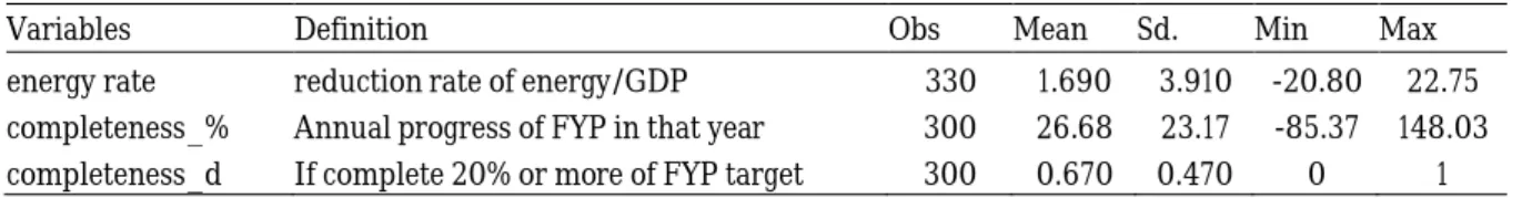
Table 3. Statistical Descriptions of Major Policy Variables.

Variables Definition Obs Mean Sd. Min Max

energy rate reduction rate of energy/GDP 330 1.690 3.910 -20.80 22.75 completeness_% Annual progress of FYP in that year 300 26.68 23.17 -85.37 148.03 completeness_d If complete 20% or more of FYP target 300 0.670 0.470 0 1 5.2 The Emission Reduction Effect of Mandatory Mitigation Policies

Firstly, we examine whether the implementation of mandatory targets has effectively reduced emissions. Mandatory targets reduce emissions not only by lowering the energy intensity, but also through other channels, such as encouraging carbon sequestration technology, encouraging research and development, and enhancing productivity as well as sending emissions reduction signals. Here the dependent variables are production-based and consumption-based emissions.

The independent variables are the different measures for the completion of mitigation targets.

With reference to the IPAT, the STRIPAT, and the Kaya models, this paper also introduces other control variables. We run the following model to test the effectiveness of mandatory targets.

𝑒𝑒_{𝑐𝑐𝑡𝑡}=𝛼𝛼+𝛽𝛽𝑋𝑋_{𝑐𝑐𝑡𝑡}+𝜃𝜃𝑍𝑍_{𝑐𝑐𝑡𝑡}+𝛾𝛾_𝑐𝑐+𝛿𝛿_𝑡𝑡+𝜀𝜀_{𝑐𝑐𝑡𝑡} (23)

where 𝑒𝑒_{𝑐𝑐𝑡𝑡} is production-based emissions or consumption-based emissions of region 𝑖𝑖 in year 𝑅𝑅.

𝑋𝑋𝑐𝑐𝑡𝑡 is the policy variable with which we are concerned. The policy variable measures the completion of mitigation targets in the given year. We consider 𝑅𝑅𝑖𝑖𝑅𝑅𝑒𝑒𝑒𝑒𝑒𝑒 𝑒𝑒𝑖𝑖𝑅𝑅𝑅𝑅, 𝑐𝑐𝑜𝑜𝑐𝑐𝑐𝑐𝑐𝑐𝑅𝑅𝑅𝑅𝑅𝑅𝑖𝑖𝑅𝑅𝑅𝑅𝑅𝑅_%, and c𝑜𝑜𝑐𝑐𝑐𝑐𝑐𝑐𝑅𝑅𝑅𝑅𝑅𝑅𝑖𝑖𝑅𝑅𝑅𝑅𝑅𝑅_𝑑𝑑 as policy variables. 𝑍𝑍_{𝑐𝑐𝑡𝑡} is a series of control variables, including the logarithm of per capita GDP, lnGDP, population, lnPopulation, urbanization rate, urbanrate, share of children, and elderly in population, old&young, GDP ratio of third industry industry_3rd, GDP ratio of imports, IM_% and exports, EX_%, and the proportion of coal in total energy consumption coalrate, which is often considered and controlled for in the previous literature.

These variables are calculated from the China Statistical Yearbook and the National Bureau of Statistics website. γ𝑐𝑐 and 𝛿𝛿𝑡𝑡 are the fixed effects of the province and time, respectively. 𝜀𝜀𝑐𝑐𝑡𝑡 is the random error term. Since key independent variables are all expressed in percentages, we calculate the logarithms of two dependent variables, consumption-based and production-based carbon emissions, respectively. We then discuss the elasticity between policy intensity and emissions. The main regression results of the total effect are shown in Table 4.

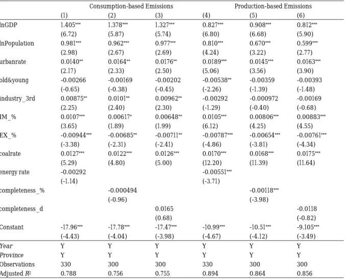
Table 4 indicates that the implementation of mandatory targets significantly reduces production-based emissions. It also has a negative, but insignificant, impact on consumption- based emissions. Regressions (1), (2) and (3) demonstrate the interrelationship between consumption-based emissions and policy implementation intensity. The results suggest that

13

mandatory targets can reduce consumption-based emissions as a vane policy. But policy implementation intensity does not result in significant reductions in consumption-based emissions. Regressions (4), (5) and (6) show the interrelationship between production-based emissions and policy implementation intensity. Since mitigation policies mainly target local enterprises and residents, we expect that the implementation of mandatory targets would reduce production-based emissions. The regressions show that: (1) for every 1% increase in the reduction rate of energy consumption per unit of GDP, production-based emissions drop by 0.551%; (2) for each 1% increase in overall completion of the mandatory target during the relevant FYP, production-based emissions decrease by 0.118%; (3) if the yearly mandatory target is completed, production-based emissions also decrease, notwithstanding insignificantly. It is worth noting that control variables like coalrate might also be influenced by mitigation policy, for instance, the policy might lower the share of coal in total energy use. However, this does not affect the basic results of our study since we might have underestimated the policy effect. As long as the mandatory target is effective under current our estimation, it shall still be effective when we further take into consideration the mediating effect of changes in industry and energy structures.

Table 4. Emission Reduction Effect of Mandatory Mitigation Policies.

Consumption-based Emissions Production-based Emissions

(1) (2) (3) (4) (5) (6)

lnGDP 1.405^*** 1.378^*** 1.327^*** 0.827^*** 0.908^*** 0.812^***

(6.72) (5.87) (5.74) (6.80) (6.68) (5.90)

lnPopulation 0.981^*** 0.962^*** 0.977^*** 0.810^*** 0.670^*** 0.599^***

(2.98) (2.67) (2.69) (4.24) (3.22) (2.77)

urbanrate 0.0140^** 0.0164^** 0.0176^** 0.0189^*** 0.0145^*** 0.0163^***

(2.17) (2.33) (2.50) (5.06) (3.56) (3.90)

old&young -0.00266 -0.00169 -0.00202 -0.00538^** -0.00359 -0.00393

(-0.65) (-0.38) (-0.45) (-2.26) (-1.39) (-1.48)

industry_3rd 0.00875^** 0.0101^** 0.00962^** -0.00292 -0.000972 -0.00169

(2.25) (2.40) (2.30) (-1.29) (-0.40) (-0.68)

IM_% 0.0107^*** 0.00617^* 0.00648^** 0.0105^*** 0.00806^*** 0.00883^***

(3.65) (1.89) (1.99) (6.12) (4.25) (4.55)

EX_% -0.00944^*** -0.00685^** -0.00711^** -0.00787^*** -0.00654^*** -0.00761^***

(-3.38) (-2.31) (-2.41) (-4.86) (-3.81) (-4.34)

coalrate 0.0127^*** 0.0122^*** 0.0126^*** 0.0170^*** 0.0168^*** 0.0175^***

(5.29) (4.80) (5.00) (12.20) (11.39) (11.64)

energy rate -0.00292 -0.00551^***

(-1.14) (-3.71)

completeness_% -0.000494 -0.00118^***

(-0.96) (-3.98)

completeness_d 0.0165 -0.0118

(0.68) (-0.82)

Constant -17.96^*** -17.78^*** -17.47^*** -10.99^*** -10.51^*** -9.105^***

(-4.43) (-4.04) (-3.98) (-4.67) (-4.12) (-3.49)

Year Y Y Y Y Y Y

Province Y Y Y Y Y Y

Observations 330 300 300 330 300 300

Adjusted R² 0.788 0.756 0.755 0.894 0.864 0.856

t statistics in parentheses

* p < 0.1, ^** p < 0.05, ^*** p < 0.01

14

5.3 The Impact Of Mitigation Policies on Emissions Transfers

This paper then examines how mitigation policies would change the provinces’ net emissions transfers. That is, for this sector, we try to test whether more emissions would outflow from the provinces with more stringent mandatory target implementation. We run the following model to test the impact of mandatory targets.

𝑒𝑒𝑐𝑐𝑡𝑡=𝛼𝛼+𝛽𝛽𝑋𝑋𝑐𝑐𝑡𝑡+𝜃𝜃𝑍𝑍𝑐𝑐𝑡𝑡+𝛾𝛾𝑐𝑐+𝛿𝛿𝑡𝑡+𝜀𝜀𝑐𝑐𝑡𝑡 (24)

Here the dependent variable, 𝑒𝑒_{𝑐𝑐𝑡𝑡}, is variable 𝑑𝑑.𝑏𝑏𝑖𝑖𝑐𝑐𝑖𝑖𝑖𝑖𝑐𝑐𝑅𝑅_{𝑐𝑐𝑡𝑡}, which indicate net emissions transfer changes in province 𝑖𝑖 in year 𝑅𝑅 as compared to last year.

𝑑𝑑.𝑏𝑏𝑖𝑖𝑐𝑐𝑖𝑖𝑖𝑖𝑐𝑐𝑅𝑅𝑐𝑐𝑡𝑡=𝑏𝑏𝑖𝑖𝑐𝑐𝑖𝑖𝑖𝑖𝑐𝑐𝑅𝑅𝑐𝑐𝑡𝑡− 𝑏𝑏𝑖𝑖𝑐𝑐𝑖𝑖𝑖𝑖𝑐𝑐𝑅𝑅𝑐𝑐𝑡𝑡−1 (25)

The independent variable 𝑋𝑋_{𝑐𝑐𝑡𝑡} still measures the implementation of mitigation targets. We consider 𝑅𝑅𝑖𝑖𝑅𝑅𝑒𝑒𝑒𝑒𝑒𝑒 𝑒𝑒𝑖𝑖𝑅𝑅𝑅𝑅, 𝑐𝑐𝑜𝑜𝑐𝑐𝑐𝑐𝑐𝑐𝑅𝑅𝑅𝑅𝑅𝑅𝑖𝑖𝑅𝑅𝑅𝑅𝑅𝑅%, and c𝑜𝑜𝑐𝑐𝑐𝑐𝑐𝑐𝑅𝑅𝑅𝑅𝑅𝑅𝑖𝑖𝑅𝑅𝑅𝑅𝑅𝑅_𝑑𝑑 as the policy variables. The lag terms of these policy variables are also considered to include the time-lag effect of mitigation policy.

Similar to previous models, we also include other controlled variables in this model as 𝑍𝑍_{𝑐𝑐𝑡𝑡}. γ_𝑐𝑐, and 𝛿𝛿𝑡𝑡 which are the fixed effects of the province and time, respectively. 𝜀𝜀𝑐𝑐𝑡𝑡 is the random error term.

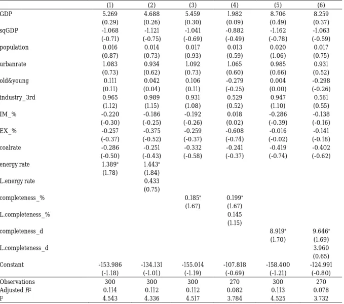
The results are presented in Table 6.

Table 5. Impact on Net Emissions Transfers.

(1) (2) (3) (4) (5) (6)

GDP 5.269 4.688 5.459 1.982 8.706 8.259

(0.29) (0.26) (0.30) (0.09) (0.49) (0.37)

sqGDP -1.068 -1.121 -1.041 -0.882 -1.162 -1.063

(-0.71) (-0.75) (-0.69) (-0.49) (-0.78) (-0.59)

population 0.016 0.014 0.017 0.013 0.020 0.017

(0.87) (0.73) (0.93) (0.59) (1.06) (0.75)

urbanrate 1.083 0.934 1.092 1.065 0.985 0.931

(0.73) (0.62) (0.73) (0.60) (0.66) (0.52)

old&young 0.111 0.042 0.106 -0.279 0.004 -0.298

(0.11) (0.04) (0.11) (-0.25) (0.00) (-0.26)

industry_3rd 0.965 0.989 0.931 0.529 0.947 0.561

(1.12) (1.15) (1.08) (0.52) (1.10) (0.55)

IM_% -0.220 -0.186 -0.192 0.018 -0.286 -0.138

(-0.30) (-0.25) (-0.26) (0.02) (-0.39) (-0.16)

EX_% -0.257 -0.375 -0.259 -0.608 -0.016 -0.141

(-0.37) (-0.52) (-0.37) (-0.74) (-0.02) (-0.18)

coalrate -0.286 -0.251 -0.332 -0.241 -0.419 -0.402

(-0.50) (-0.43) (-0.58) (-0.37) (-0.74) (-0.62)

energy rate 1.389^* 1.443^*

(1.78) (1.84)

L.energy rate 0.433

(0.75)

completeness_% 0.185^* 0.199^*

(1.67) (1.67)

L.completeness_% 0.145

(1.15)

completeness_d 8.919^* 9.646^*

(1.70) (1.69)

L.completeness_d 3.960

(0.65)

Constant -153.986 -134.131 -155.014 -107.818 -158.400 -124.991

(-1.18) (-1.01) (-1.19) (-0.69) (-1.21) (-0.80)

Observations 300 300 300 270 300 270

Adjusted R² 0.114 0.112 0.112 0.082 0.113 0.078

F 4.543 4.336 4.517 3.784 4.525 3.732

z statistics in parentheses

* p < 0.1, ^** p < 0.05, ^*** p < 0.01

15

The results reveal that the implementation of mandatory targets has a significant impact on a province’s net emissions transfer. Under stricter mitigation policies, a province will transfer more of their emissions to other areas. Specifically, the higher the energy intensity reduction rate, the higher the completion share of the mandatory target, as well as the completeness of the target as measured by a dummy variable, which all contribute to the overall increase in net emissions transfers. This implies that stringent mitigation policy encourages a net emissions outflow and induces the carbon leakage embodied in inter-provincial trade.

6. The Effectiveness of Implementation Intensity of Mitigation Targets

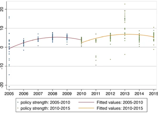
Establishing mandatory mitigation targets can efficiently obtain expected goals in the short term. One flaw of such short-term targets is that once the goal is achieved, governments may no longer have the incentive to continue policy implementation. For example, in the FYP, before mitigation targets are realized, provincial governments tend to strengthen policy implementation to accomplish mandatory targets on time and avoid administrative accountability. However, if the government completes the FYP target in advance, it has no further incentive to maintain stringent mitigation policies during the remaining years of the relevant FYP. By doing this, the local government can ease the negative pressure of mitigation on the economy and living standards.

Meanwhile, it leaves enough room for the successful completion of the next FYP’s targets. This leads to a weaker implementation of mitigation policies in the remaining years of the FYP.

To test this hypothesis, this study examines the implementation patterns of mitigation policies, that is, we investigate how stringency changes over time. We use three indicators for policy implementation intensity: 𝑅𝑅𝑖𝑖𝑅𝑅𝑒𝑒𝑒𝑒𝑒𝑒 𝑒𝑒𝑖𝑖𝑅𝑅𝑅𝑅, 𝑐𝑐𝑜𝑜𝑐𝑐𝑐𝑐𝑐𝑐𝑅𝑅𝑅𝑅𝑅𝑅𝑖𝑖𝑅𝑅𝑅𝑅𝑅𝑅_𝑑𝑑, and 𝑐𝑐𝑜𝑜𝑐𝑐𝑐𝑐𝑐𝑐𝑅𝑅𝑅𝑅𝑅𝑅𝑖𝑖𝑅𝑅𝑅𝑅𝑅𝑅_% as independent variables. We use two models to test for changes in policy stringency. First, we use a dummy variable 𝑐𝑐.𝑐𝑐𝑜𝑜𝑐𝑐𝑐𝑐𝑐𝑐𝑅𝑅𝑅𝑅𝑅𝑅𝑖𝑖𝑅𝑅𝑅𝑅𝑅𝑅_𝑑𝑑 to test whether achievement of the mandatory target in a previous year would weaken stringency in the following year. Second, we also use the ordinal of that year in the corresponding FYPs, 𝑅𝑅 and its quadratic terms 𝑅𝑅𝑠𝑠𝑅𝑅 to test for the stringency change in mitigation policy. Other controlled variables are also included in the model. The regression model is as follows.

𝑒𝑒𝑐𝑐𝑡𝑡=𝛼𝛼+𝛽𝛽𝑋𝑋𝑐𝑐𝑡𝑡+𝛽𝛽2𝑅𝑅𝑐𝑐𝑡𝑡+𝛽𝛽3𝑅𝑅𝑠𝑠𝑅𝑅𝑐𝑐𝑡𝑡+𝛾𝛾𝑐𝑐+𝜀𝜀𝑐𝑐𝑡𝑡 (26) 𝑒𝑒_{𝑐𝑐𝑡𝑡}=𝛼𝛼+𝛽𝛽𝑋𝑋_{𝑐𝑐𝑡𝑡}+𝛽𝛽₁𝑐𝑐.𝑐𝑐𝑜𝑜𝑐𝑐𝑐𝑐𝑐𝑐𝑅𝑅𝑅𝑅𝑅𝑅𝑖𝑖𝑅𝑅𝑅𝑅𝑅𝑅_𝑑𝑑_{𝑐𝑐𝑡𝑡}+𝛾𝛾_𝑐𝑐+𝜀𝜀_{𝑐𝑐𝑡𝑡} (27)

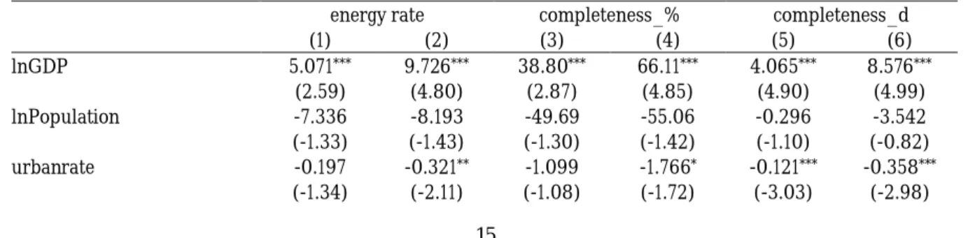
Regressions (1) and (2) test energy rate reductions. Regressions (3) and (4) concern the completeness progress for each year. And regressions (5) and (6) test whether 20% or more of the total target is completed (or not) as the dependent variable, using the random effect model and Probit regression. Results are shown in Table 6.

Table 6. The Effectiveness of Mitigation Policy after the Achievement of FYP Targets.

energy rate completeness_% completeness_d

(1) (2) (3) (4) (5) (6)

lnGDP 5.071^*** 9.726^*** 38.80^*** 66.11^*** 4.065^*** 8.576^***

(2.59) (4.80) (2.87) (4.85) (4.90) (4.99)

lnPopulation -7.336 -8.193 -49.69 -55.06 -0.296 -3.542

(-1.33) (-1.43) (-1.30) (-1.42) (-1.10) (-0.82)

urbanrate -0.197 -0.321^** -1.099 -1.766^* -0.121^*** -0.358^***

(-1.34) (-2.11) (-1.08) (-1.72) (-3.03) (-2.98)