JAIST Repository: Stability analysis of underactuated compass gait based on linearization of motion

Japan Advanced Institute of Science and Technology

https://dspace.jaist.ac.jp/

Title

Stability analysis of underactuated compass gait

based on linearization of motion

Author(s)

Asano, Fumihiko

Citation

Multibody System Dynamics, 33(1): 93-111

Issue Date

2014-04-02

Type

Journal Article

Text version

author

URL

http://hdl.handle.net/10119/15455

Rights

This is the author-created version of Springer,

Fumihiko Asano, Multibody System Dynamics, 33(1),

2014, 93-111. The original publication is

available at www.springerlink.com,

http://dx.doi.org/10.1007/s11044-014-9416-9

Description

(will be inserted by the editor)

Stability analysis of underactuated compass gait

based on linearization of motion

Fumihiko Asano

Received: date / Accepted: date

Abstract This paper investigates the stability principle underlying an

un-deractuated compass gait generated by strict output following control of the hip-joint angle. First, we introduce a planar underactuated compass-like biped robot with semicircular feet and develop its mathematical model. We then lin-earize the equation of motion and design an output following control for the relative hip-joint angle of the linearized model. Second, we analytically derive the transition function of the state error for the stance phase based on the state space representation and discuss its physical meaning. We also mathe-matically show that the collision phase is always stable. Finally, the validity of the theoretical results is verified through numerical simulations.

Keywords Limit cycle walking· Stability · Convergence rate · Compass gait

1 Introduction

Limit cycle walking inspired by McGeer’s passive dynamic walking [1][2] uti-lizes the robot’s own dynamics and the inherent stability of the periodic or-bit, and has been actively studied as an effective way for achieving natural and energy-efficient robotic legged locomotion [3][4]. Unlike walkers that are controlled concerning the zero moment point (ZMP) [5], limit cycle walkers in most cases generate a stable level gait without using ankle-joint torques by adjusting the system parameters or by following suitably-designed time-dependent trajectories except those for the ankle joints. Stability guarantee is therefore an important issue in the control design and several methods for F. Asano

School of Information Science, Japan Advanced Institute of Science and Technology 1-1 Asahidai, Nomi, Ishikawa 923-1292, Japan

Tel.: +81-761-51-1243 Fax: +81-761-51-1149 E-mail: fasano@jaist.ac.jp

analyzing the stability of the generated gait have been proposed [6][7]. Dy-namic gait generation for limit cycle walkers is, however, still trial-and-error method and we must always carefully adjust the system parameters with the expectation that the generated gait would be stabilized while walking.

It is well known that a passive rimless wheel always generates 1-period and asymptotically stable walking gaits regardless of the given slope angle [1][8]. This stability principle is obvious and can be easily explained by using a simple recurrence formula of kinetic energy immediately before impact [9]. The authors applied this mechanism to a fully-actuated biped robot and achieved asymptotically stable bipedal locomotion by satisfying two conditions; one is the constraint on impact posture and the other is that on restored mechanical energy [10]. These conditions are those for walkers to discretely behave in the same manner as a rimless wheel. The robot must be, however, fully-actuated to satisfy both conditions simultaneously. Especially, ankle-joint actuation is necessary for controlling the restored mechanical energy. We must recognize, however, that achieving stable walking for fully-actuated walkers is not difficult in this case because they can be controlled as a robotic arm fixed on the floor. The most difficult aspect for understanding the gait stability rests on underactuation or uncontrollability of the ankle joints, and that is why the inherent stability must be discussed.

To understand the stability underlying the generated gait, it is always required to derive the Poincar´e return map. The accuracy of the return map numerically obtained, however, significantly varies according to the method for calculating [6]. It is also difficult to understand the physical meaning underly-ing the numerical solution. Analytical solution to the return map is therefore necessary to solve the above problems. Coleman first succeeded to derive the analytical solution to the return map in a passive rimless wheel [8]. He de-rived the one-dimensional return map for the stance and the collision phases by reducing the state transition matrices using projection vectors. By apply-ing Coleman’s method, the author clarified that a stable passive compass gait consists of unstable stance phases and marginally stable collision phases [11]. The rigorous proof of the instability of the stance phase, however, has been left as a problem unsolved due to the complexity of the transition matrix.

If an underactuated bipedal walker is controlled to achieve constraint on impact posture or to fall down as a 1-DOF rigid body in the same posture immediately before every impact, the Poincar´e return map can be reduced to a one-dimensional one [7]. Then the gait stability can be clearly determined only by calculating the magnitude of the scalar transition function of the angular velocity error immediately before or immediately after impact from one to the next. From this, an underactuated bipedal gait with constraint on impact posture is the most mathematically tractable example for stability analysis based on the Poincar´e return map.

Based on the observations, this paper extends the method for stability anal-ysis based on the linearized equation of motion [11] to an active limit cycle walker strictly-controlled to follow the desired-time trajectory of the relative hip angle. We mainly address the following two subjects; one is deriving the

transition functions of the state error not by numerically but by analytically, and the other is clarifying the change in the convergence mode with the in-crease of the desired settling time by using the derived transition functions. We consider an underactuated compass-like biped robot with semicircular feet for analysis. We first derive the transition function of the state error for the stance phase and discuss the physical meaning through simplification of it. Second, we mathematically show that the collision phase is always stable re-gardless of the physical parameters. Finally, the validity of the theoretical results is investigated through numerical simulations. Note that, in this paper, the transition functions are given as scalar ones. The stability of each phase is therefore defined in terms of the reduction of the state error norm during the phase and can be determined only by calculating the magnitude of the transition functions as in the case of the Poincar´e return map.

This paper is organized as follows. Section 2 describes the mathematical model of the underactuated biped treated in this paper. Section 3 describes the linearization of motion and state space realization of the dynamics incor-porating the applied output following control. Section 4 analyzes the stability of the stance phase and Section 5 shows the stability of the collision phase. Section 6 analyzes the changes in the gait properties from the viewpoint of the convergence rate through theoretical and numerical investigations. Finally, Section 7 concludes this paper and describes future research directions.

2 Underactuated compass-like biped robot with semicircular feet

2.1 Equation of motion

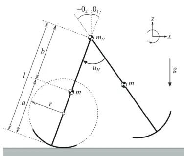
Fig. 1 shows the model of a planar, underactuated bipedal walker with semi-circular feet. This consists of two rigid leg frames with semisemi-circular feet whose radius is r [m] and three point masses. Let θ1 and θ2 be the angular positions

of the stance and swing legs with respect to vertical. Let θ =[θ1θ2

]T

be the generalized coordinate vector, the robot equation of motion then becomes

M (θ)¨θ + C(θ, ˙θ) ˙θ + g(θ) = SuH, (1)

where uH is the hip-joint torque and S =[1−1]T. The other terms in Eq. (1) are detailed as follows.

M (θ) = [ M11M12 M21M22 ] , C(θ, ˙θ) = [ C11C12 C21 0 ] M11= m ( r2+ (a− r)2+ 2r(a− r) cos θ1 ) +(mH+ m)(r2+ (l− r)2+ 2r(l− r) cos θ1 ) M12= M21=−mb (r cos θ2+ (l− r) cos θH) M22= mb2

θ1 −θ2 mH m m uH g r a b l X Z +

Fig. 1 Model of planar underactuated compass-like biped robot with semicircular feet

C11=−mr(a − r) ˙θ1sin θ1− (mH+ m)r(l− r) ˙θ1sin θ1 C12= mb ˙θ2(r sin θ2− (l − r) sin θH) C21= mb(l− r) ˙θ1sin θH g(θ) = [ − (mHl + ml + ma− Mr) g sin θ1 mbg sin θ2 ]

Here, θH := θ1−θ2[rad] is the relative hip angle and M := mH+2m [kg] is the

robot’s total mass. We assume that the rolling constraint condition between the sole and the ground always holds, that is, the foot does not slip. Then the robot can exhibit efficient level dynamic walking only by hip-joint actuation using the effects of semicircular feet; the rolling effect during the stance phase is equivalent to the ankle-joint actuation and the shock relaxation effect at impact strongly helps to reduce the energy consumption [4].

2.2 Collision equations

The relation between the angular positions immediately before impact and those immediately after impact is simply given by

θ+= [ 0 1 1 0 ] θ−, (2)

where the superscripts “−” and “+” denote immediately before and immedi-ately after impact. Here, we define the half inter-leg angle at impact as

α := θ − 1 − θ−2 2 = θ+₂ − θ₁+ 2 > 0. (3)

In this paper, we assume that α is strictly controlled to the desired value, α∗, at every impact where the superscript “∗” denotes that the variable is of the stationary orbit (steady walking gait). The relation between angular velocities immediately before impact and those immediately after impact is given by

˙θ+= Ξ(α∗) ˙θ−, (4)

where Ξ(α∗)∈ R2×2 _{is a function matrix of α}∗_{and is uniquely determined by}

the robot’s physical parameters. We assume that the hip joint is also mechan-ically locked at impact, that is, ˙θ+_H = 0 holds so that the closed system does not contain the tracking error as described later. By adding this condition, the matrix rank of Ξ(α∗) becomes one; the form is

Ξ(α∗) = [ N1/D N2/D N1/D N2/D ] , (5)

where N1, N2 and D are detailed as follows.

N1= ma2− mal + r(mb + Mr) + r(3ma + (2mH+ m)l− 2Mr) cos α∗ +(l− r)(2ma + mHl− Mr) cos(2α∗)

N2= mb(r− a − r cos α∗)

D = 2ma2+ M l2− 2rl(mH+ m) + 2M r2− 2ma(l + r)

−2mb(l − r) cos(2α∗_{) + 2r(2ma + mHl− Mr) cos α}∗

3 Linearization of motion and output following control

3.1 State space realization

By linearizing the dynamic equation (1) around the equilibrium point, θ = ˙θ = 02×1, we get

M0¨θ + G0θ = SuH. (6)

The matrices are detailed as

M0= [ mHl2+ ma2+ ml2−mbl −mbl mb2 ] , G0= [ −(mHl + ma + ml− Mr) 0 0 mb ] g.

We choose the robot’s relative hip angle, θH = STθ, as the control output

and synthesize the controller that achieves θH → θHd(t). The second order derivative of θH with respect to time becomes

¨

θH= STθ = S¨ TM−10 (SuH− G0θ) . (7)

Note that the following term

STM−1₀ S = mHl

2_{+ 2ma}2 mb2_(m

Hl2+ ma2)

is a positive scalar. A proportional-derivative (PD) feedback control is not needed because of the assumption of mechanical lock of the hip joint at impact. Then we can consider the following control input for achieving θH ≡ θHd(t).

uH = ¨

θHd(t) + STM−10 G0θ

STM−1₀ S (9)

By substituting this into Eq. (6) and arranging it, we get

M0θ +¨ ( I2− SSTM−1₀ STM−1₀ S ) G0θ = S ¨θHd(t) STM−1₀ S. (10)

Define x :=[θTθ˙T]T, the state space realization of Eq. (10) then becomes ˙ x = Ax + B ¨θHd(t), (11) where A :=   02×2 I2 −M−1 0 ( I2−SS T_M−1 0 ST M−10 S ) G0 02×2   , B := [ 02×1 M−10 S ST M−10 S ] . (12)

Matrix A and vector B have the following forms.

A =     0 0 1 0 0 0 0 1 A31 A320 0 A31 A320 0     , B =     0 0 B3 B3− 1     . (13)

A31, A32 and B3 are also detailed as A31= (mHl + ma + ml− Mr) g mHl2+ 2ma2 , A32= −mbg mHl2+ 2ma2 , B3= −mab mHl2+ 2ma2 .

The third row of A becomes equal to the fourth because of the following reason. By extracting the third and fourth rows from Eq. (11), we get

¨ θ = [ 1 1 ] [ A31A32 ] θ + M −1 0 S STM−1₀ S ¨ θHd(t). (14)

By multiplying both sides by ST, the left-hand side becomes ¨θH. The second term of the right-hand side becomes ¨θHd(t), and thus the first term of the right-hand side must become zero; this is obvious because[1 1]Tis perpendicular to S. In the case that ¨θH ≡ ¨θHd(t) does not hold and the tracking error remains, the above condition is not satisfied because the terms of PD feedback are added to matrix A. The state error system becomes more complicated.

If the collision for stance-leg exchange occurs at t = 0 [s], the solution of Eq. (11) becomes

x(t) = eAtx(0+) + ∫ t

0+

In addition, following Eqs. (2) and (4), the transition function for stance-leg exchange is summarized as x(0+) = Rx(0−), R :=   [ 0 1 1 0 ] 02×2 02×2 Ξ(α∗)   . (16) 3.2 Desired-time trajectory

The desired-time trajectory for the relative hip angle, θHd(t), is designed as follows. We introduce the following fifth-order function of time:

θHd(t) =

5

∑ k=0

aktk (17)

to smoothly move θH from−2α∗to 2α∗ during the stance phases. Let Tset[s]

be the desired settling-time, and the boundary conditions are chosen as

θHd(0+) =−2α∗, θHd(Tset) = 2α∗, ˙ θHd(0+) = ˙θHd(Tset) = 0, ¨ θHd(0+) = ¨θHd(Tset) = 0.

The desired-time trajectory is then determined as follows.

θHd(t) =    24α∗ T5 set t5−60α ∗ T4 set t4+40α ∗ T3 set t3− 2α∗(0≤ t < Tset) 2α∗ (t≥ Tset)

3.3 Typical walking gaits

Fig. 2(a) shows the simulation result of level dynamic walking of the nonlinear model where α∗ = 0.20 [rad] and Tset= 0.70 [s]. The robot’s physical

param-eters are chosen as listed in Table 1. Fig. 2(b) shows that of the linearized model in the same parameter settings. We can see that the relative hip angle is successfully controlled from−2α∗to 2α∗during the stance phases and that the linearized model exhibits almost the same motion as that of the nonlinear model. The approximation accuracy is much higher than that of passive com-pass gait [11]. This is achieved because the zero dynamics is reduced to just 1-DOF by applying the strict output following control.

-0.4 -0.3 -0.2 -0.1 0 0.1 0.2 0.3 0.4 0 0.5 1 1.5 2 2.5 3

Angular position [rad]

Time [s] _θ

1 θ2 θH

(a) Nonlinear model

-0.4 -0.3 -0.2 -0.1 0 0.1 0.2 0.3 0.4 0 0.5 1 1.5 2 2.5 3

Angular position [rad]

Time [s] _θ

1 θ2 θH

(b) Linearized model

Fig. 2 Simulation results for level dynamic walking of nonlinear and linearized biped models

where α∗= 0.20 [rad] and Tset= 0.70 [s]

Table 1 Physical parameter settings

mH 10.0 kg m 5.0 kg a 0.5 m b 0.5 m l (= a + b) 1.0 m r 0.5 m

4 Stability of stance phase

4.1 Basic definitions

– Let i (≥ 0) be the step number.

– The robot starts walking from the impact posture; this is defined as the 0th

impact. The next heel-strike collision is the first impact. The subsequent collisions are contextually counted.

– Let ti [s] be the absolute time of the (i)th collision. The (i)th step period is defined as Ti:= ti+1− ti [s].

– The state vectors immediately before and immediately after impact, x(t−_i ) and x(t+_i), are simply denoted as x−_i and x+_i .

– The subscript “eq” denotes that the state variable or the state vector are

of the equilibrium point on the Poincar´e section.

4.2 Derivation of state error system

The state vector immediately before the (i + 1)th impact, x−_i+1, is written by that immediately after the (i)th impact, x+_i , as

x−_i+1= eATi_x+

i + ∫ T_i−

0+

eA(Ti−s)_{B ¨θHd(s)ds. (18)}

By considering that ¨θHd(s) = 0 holds when s≥ Tset, Eq. (18) can be arranged

as x−_i+1= eATi_x+ i + ∫ Tset 0+ eA(Ti−s)_{B ¨θHd(s)ds. (19)} Here, define η := ∫ Tset 0+ e−AsB ¨θHd(s)ds, (20) Eq. (19) is then rearranged as

x−_i+1= eATi(_x+

i + η )

. (21)

In a steady gait, the following equation

x−_eq= eAT∗(x+_eq+ η) (22)

should hold. Let ∆x−_i be the state error vector immediately before the (i)th impact, that is, x−_i = x−_eq+ ∆x−_i . The state vector immediately before the (i + 1)th impact is then written as

x−_i+1 = eA(T∗+∆Ti)_(x+ eq+ ∆x + i + η) = eA∆Ti_eAT∗_(x+ eq+ η) + e A∆Ti_eAT∗_∆x+ i = eA∆Ti_x− eq+ e A∆Ti_eAT∗_∆x+ i . (23)

Here, we used the relation of Ti = T∗+ ∆Ti. By using an approximation of eA∆Ti ≈ I

4+ A∆Ti and ignoring the error terms higher than second order,

Eq. (23) is further approximated as

x−_i+1≈ x−_eq+ Ax−_eq∆Ti+ eAT

∗

∆x+_i . (24)

Define

and multiplying x by p leads to px = θ1+ θ2. This geometrically denotes the

double volume of the hip-angle bisector, and heel-strike collision occurs when the value reaches zero from negative. At this instant, the relation px−_i =

px−eq= α∗− α∗= 0 holds. Note that, however, the projection vector p is not

unique in the case that the robot falls down as a 1-DOF rigid body. Eq. (25) is one of the necessary conditions.

By multiplying both sides of Eq. (24) by p, we get 0 = pAx−eq∆Ti+ peAT ∗ ∆x+_i . (26) ∆Ti is then solved as ∆Ti=− peAT∗_∆x+ i pAx−eq . (27)

Note that the denominator is

pAx−_eq= ˙θ−_1eq+ ˙θ−_2eq= 2 ˙θ−_1eq

and this is not zero (positive). By substituting Eq. (27) into Eq. (24) and considering the relation of ∆x−_i+1 = x−_i+1− x−_eq, the transition matrix of the state error is finally derived as

∆x−_i+1= Q∆x+_i , Q := ( I4− Ax−_eqp pAx−eq ) eAT∗. (28)

This is a four-dimensional redundant map and is reduced as follows. The state error vector has the form

∆x±_i =      0 0 ∆ ˙θ±_1(i) ∆ ˙θ±_1(i)     = v∆ ˙θ ± 1(i), v :=     0 0 1 1     , (29)

and the following relation

∆ ˙θ±_1(i)= 1 2v

T_∆x±

i (30)

holds. Eq. (28) is then reduced to

∆ ˙θ−_1(i+1)= ¯Q∆ ˙θ+_1i, Q :=¯ 1

2v

T_{Qv, (31)}

where the equation ¯Q is detailed as

¯ Q = cosh (ζT∗)−α ∗_{(A31− A32) sinh (ζT}∗₎ ζ ˙θ−_1eq , (32) ζ :=√A31+ A32= √ M (l− r) − 2mb mHl2+ 2ma2 g. (33)

ζ can be defined if the relation

l > r +2mb

M (34)

4.3 Physical meaning of ¯Q

The author showed that, in passive dynamic walking of a rimless wheel, the transition matrix of the state error for the stance phase can be reduced to a scalar function, ¯Q, without including the steady step period [9]. To clearly

understand the physical meaning of ¯Q, we apply the same approach in the

following. Define x′_i:= x+_i + η =     θ′_1i θ′_2i ˙ θ′_1i ˙ θ′_2i     , (35) x′eq:= x+eq+ η =      θ′_1eq θ′2eq ˙ θ′_1eq ˙ θ′_2eq     , (36)

then Eqs. (21) and (22) can be rewritten as

x−_i+1= eATi_x′

i, (37)

x−eq= eAT

∗

x′eq. (38)

These represent the state transitions in the linear system ˙

x = Ax (39)

where the initial conditions are x′_i or x′_eq. By extracting the third and fourth rows of Eq. (39), we get

¨

θ1= ¨θ2= A31θ1+ A32θ2. (40)

This comes from the special form of A in Eq. (13). In addition, this equa-tion implicitly expresses passivity and is important to simplify the transiequa-tion function as described later.

Eqs. (37) and (38) can be equivalently written as

x′_i= e−ATi_x−

i+1, (41)

x′_eq= e−AT∗x−_eq. (42)

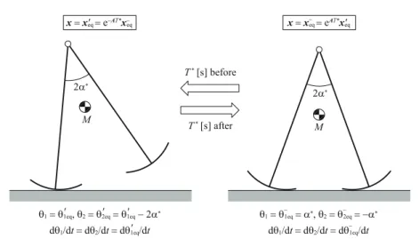
Then we can understand that the vectors x′_iand x′_eqare the conditions (pos-tures) going back to Tior T∗[s] before remaining in a 1-DOF rigid body from those immediately before impact, x−_i and x−_eq. This is explained in a little more detail as follows. The robot moves backward through time from the im-pact posture immediately before imim-pact, θ−_1eq=−θ−_2eq= α∗ and ˙θ−_1eq = ˙θ−_2eq

dynamics maintains the relation ¨θ1= ¨θ2. Since the robot starts from the

con-dition where the both angular velocities are the same, it moves as a 1-DOF rigid body whose relative hip angle is 2α∗. Therefore, we can conclude that the vectors x′eq and η in Eq. (36) should have the following forms

x′_eq=      θ_1eq′ θ′_1eq− 2α∗ ˙ θ′_1eq ˙ θ′_1eq     , η =     η1 η2 η3 η4     , (43) η2= η1− 2α∗, η3= η4. (44)

This can be also shown by analytically calculating Eq. (20), but the elements are fairly complex formulas and we omit the details (only η3is described later).

Eq. (38) is detailed and arranged as      θ−_1eq −θ− 1eq ˙ θ−1eq ˙ θ−_1eq     =     2ζ−2A32θ1eq− −2ζ−2_A 31θ−1eq 0 0     +      βζ−2 βζ−2 ˙ θ′1eq ˙ θ′_1eq     cosh(ζT∗) +      ζ−1θ˙′_1eq ζ−1θ˙′1eq βζ−1 βζ−1     sinh(ζT∗). (45) By reducing the redundancy of this equation, we can rearrange it to

[ β ζ ˙θ′_1eq ζ2_θ˙′ 1eq βζ ] [ cosh (ζT∗) sinh (ζT∗) ] = [ (A31− A32) θ−1eq ζ2θ˙−_1eq ] , (46) where β := ζ2θ_1eq′ − 2A32θ1eq− .

By solving Eq. (46), we can obtain cosh (ζT∗) and sinh (ζT∗) as functions without including T∗. Substituting them into Eq. (32) and rearranging it lead to ¯ Q = ˙ θ′_1eq ˙ θ−_1eq· (A31+ A32) ( ˙ θ−_1eq )2 −(A31θ−1eq+ A32θ2eq− )2 (A31+ A32) ( ˙ θ′_1eq )2 −(A31θ′1eq+ A32θ2eq′ )2. (47)

We then simplify this function. Let us define

F (x) := (A31+ A32) ˙θ 2

1− (A31θ1+ A32θ2) 2

, (48)

and we show that this is constant. Time derivative of F (x) becomes dF (x) dt = 2 (A31+ A32) ˙θ1 ¨ θ1− 2 (A31θ1+ A32θ2) ( A31θ˙1+ A32θ˙2 ) . (49)

2α∗ 2α∗ M M T* _{[s] before} T* _{[s] after} x = x'_{eq = e}−AT*_x− eq x = x − eq = eAT*x'eq

θ1 = θ'1eq, θ2 = θ'2eq = θ'1eq − 2α∗

dθ1/dt = dθ2/dt = dθ'1eq/dt θ1 = θ − 1eq = α∗, θ2 = θ − 2eq = −α∗ dθ1/dt = dθ2/dt = dθ − 1eq/dt

Fig. 3 Relation between condition immediately before impact and that where x = x′_eq

By considering that the robot moves from x−_eq to x′_eq while maintaining the relation ˙θ1= ˙θ2 and ¨θ1= ¨θ2, Eq. (49) can be arranged as follows.

dF (x) dt = 2 (A31+ A32) ˙θ1 ¨ θ1− 2 (A31θ1+ A32θ2) (A31+ A32) ˙θ1 = 2 ˙θ1(A31+ A32) ( ¨ θ1− (A31θ1+ A32θ2) ) = 0

The last equality comes from Eq. (40). Therefore we can conclude

(A31+ A32) ( ˙ θ−_1eq )2 −(A31θ1eq− + A32θ−2eq )2 (A31+ A32) ( ˙ θ′_1eq )2 −(A31θ1eq′ + A32θ′2eq )2 = 1.

Eq. (47) then finally becomes

¯ Q = ˙ θ′_1eq ˙ θ−1eq . (50)

This is written as a simple ratio of the steady angular velocities shown in Fig. 3. If ˙θ′_1eq can be controlled to zero, ¯Q then becomes zero and this implies

that the generated gait converges to the steady motion through a single step as described later. In this case, the gait stability is optimized in terms of convergence rate.

5 Stability of collision phase

5.1 Derivation of state error system

The state vector immediately after impact is written as

x+_i = Rx−_i = R(x−eq+ ∆x−i ) . (51) By considering x+ eq= Rx−eqand ∆x + i = x +

i − x+eq, the transition equation for

the state error vector is obtained as

∆x+_i = R∆x−_i . (52)

By considering Eqs. (29) and (30), Eq. (52) can be reduced to

∆ ˙θ+_1i= ¯R∆ ˙θ−_1i, R :=¯ 1

2v

T_{Rv. (53)}

By extracting the essential part from ¯R, it is rewritten as

¯ R = 1 2 [ 1 1 ]T Ξ(α∗) [ 1 1 ] = N1+ N2 D . (54) 5.2 Stability of ¯R

The eigenvalues of matrix Ξ(α∗) are 0 and (N1+ N2)/D. The sufficient

con-dition for the stability of the collision phase is then specified as 

N1+ N2 D

 < 1, (55)

and this is equivalent to

(N1+ N2)2− D2=−2M(l − r)2sin2α∗G < 0, (56)

or G > 0 because 2M (l− r)2_sin2_{α∗> 0. G is detailed as} G := 4m(a2− a(l + r) + lr)+ M (l2− 2lr + 3r2)

+(l− r)(mHl− 2ml + 4ma − Mr) cos(2α∗)

+4r(mHl + 2ma− Mr) cos α∗. (57) We will show that G is always positive regardless of the foot radius, r, in the following. Derivative of G with respect to r becomes

∂G ∂r = 8(M r(1− cos α ∗_{) + mHl + 2ma) sin}2 ( α∗ 2 ) ,

and this is always positive. G is thus found to be a monotonically increasing function. Besides,

G0:= G|r=0= ml

where β := a/l [-] and γ := mH/m [-]. Their ranges of value are 0 ≤ β ≤ 1

and 0≤ γ ≤ ∞. G0can be deformed to the following positive function: G0= 4ml2 ( β−1− cos(2α ∗₎ 2 )2 + 2ml2cos2α∗(γ + 2 sin2α∗) > 0. This shows that G monotonically increases with respect to r from the positive initial value G0, that is, G is always positive for all r (≥ 0). This gives proof

that the inequality (55) holds, that is, the collision phase is stable.

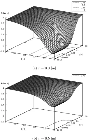
Fig. 4 plots the value of ¯R with respect to β and γ for two values of the foot

radius, r. Note that γ is plotted in logarithmic scale. These plots support that  ¯R< 1 is satisfied in all range. From Fig. 4 (a), we can see that ¯R becomes

negative where both β and γ are sufficiently small. It is also seen that ¯R in

Fig. 4 (b) are larger than those in (a) in all range. ¯R is large (close to 1.0)

means that shock-absorbing effect is high [4]. This is achieved by choosing r as a large value. Especially, ¯R reaches 1.0 as r → l or β → 1.0. In this case,

kinetic energy does not dissipate at impact.

1e-05 0.0001 0.001 0.01 0.1 1 10 0 0.2 0.4 0.6 0.8 1 -0.2 0 0.2 0.4 0.6 0.8 1 R-bar [-] 0.75 0.5 0.25 0 γ [-] β [-] R-bar [-] (a) r = 0.0 [m] 1e-05 0.0001 0.001 0.01 0.1 1 10 0 0.2 0.4 0.6 0.8 1 -0.2 0 0.2 0.4 0.6 0.8 1 R-bar [-] 0.75 γ [-] β [-] R-bar [-] (b) r = 0.5 [m]

6 Gait analysis

6.1 Three convergence modes and effect of Tset

As discussed in the previous section, ¯R becomes a positive constant in most

cases if the walker achieves a constraint on impact posture. The convergence rate of the state error is then able to be changed only by controlling ¯Q. This

section then discusses how ¯Q changes with respect to Tsetfor the output

fol-lowing control.

In [1], McGeer called the convergence property of 0 < ¯Q ¯R < 1 the speed

mode. In this case, the state error ∆ ˙θ−_1(i) monotonically converges to zero without vibrating. He also called the convergence property of−1 < ¯Q ¯R < 0

the totter mode. In this case, the state error vibrationally converges to zero. In the middle mode, ¯Q ¯R = 0, the state error is settled to zero through a single

step and this gives the optimal solution in terms of convergence rate. In this sense, this mode should be termed as the deadbeat mode.

In this section, we deal with the same biped model as in section 3. The physical parameters are chosen as listed Table 1. The foot radius is r = 0.5 [m] and ¯R is always positive as discussed in the previous section. Therefore

the sign of ¯Q ¯R is the same as that of ¯Q.

Where Tset= 0, η3becomes zero and this is obvious from the definition of η in Eq. (20). In this case, ¯Q accordingly becomes

¯ Q_T set=0 = ˙ θ+_1eq ˙ θ−_1eq . (58)

This is positive because both ˙θ+_1eqand ˙θ−_1eqmust be positive in a stable walking gait. In addition, this is less than 1 or the stance phase is stable because the angular velocity always decreases at impact, that is, ˙θ+_1eq< ˙θ−_1eqholds.

η3 in Eq. (43) is detailed as η3=− 480α∗ ζ6_T5 set (A31B3+ A32(B3− 1)) sinh ( ζTset 2 ) ×((12 + ζ2T_set2 )sinh ( ζTset 2 ) − 6ζTsetcosh ( ζTset 2 )) . (59) The partial derivative of η3 with respect to Tsetbecomes

∂η3 ∂Tset =−240α ∗ ζ6_T6 set (A31B3+ A32(B3− 1)) H(Tset), (60) where H(Tset) = 3 ( 20 + ζ2Tset2 ) − 3(20 + 3ζ2Tset2 ) cosh (ζTset) +ζTset ( 36 + ζ2Tset2 ) sinh (ζTset) , (61)

A31B3+ A32(B3− 1) =

mbg (mHbl + M aR)

(mHl2_{+ 2ma}2₎2 > 0. (62) η3then monotonically decreases as Tsetincreases if H(Tset) > 0 holds. We will

prove that this is true in the following.

For simplicity, in the following we will denote the partial derivative of

H(Tset) with respect to Tsetas

H′(Tset) :=

∂H(Tset) ∂Tset

.

The first-, second- and third-order partial derivatives of H(Tset) with respect

to Tsetbecome

H′(Tset) = 6ζ2Tset+ ζ2Tset

(

18 + ζ2T_set2 )cosh (ζTset)

−6ζ(4 + ζ2T_set2 )sinh (ζTset) , (63) H′′(Tset) = 6ζ2− 3ζ2

(

2 + ζ2T_set2 )cosh (ζTset)

+ζ3Tset

(

6 + ζ2T_set2 )sinh (ζTset) , (64) H′′′(Tset) = ζ6Tset3 cosh (ζTset) > 0. (65)

Where Tset= 0, H(Tset) and its partial derivatives become

H(0) = 0, (66)

H′(0) = 0, (67)

H′′(0) = 0. (68)

Eqs. (65) and (68) give proof of

H′′(Tset) > 0. (69)

In the same way, Eqs. (67) and (69) give proof of

H′(Tset) > 0. (70)

Furthermore, Eqs. (66) and (70) give proof of H(Tset) > 0. Therefore we can

conclude that Eq. (60) is always negative and η3 monotonically decreases as Tsetincreases. It is then expected that the numerator of ¯Q,

˙

θ′_1eq:= ˙θ+_1eq+ η3, (71)

monotonically decreases as Tset increases unless ˙θ +

1eq exhibits a significant

change. This implies that ¯Q (or ¯Q ¯R) would monotonically decrease from

posi-tive to negaposi-tive. In other words, the convergence property would change from the speed mode to the totter mode through the deadbeat mode.

6.2 Analysis results

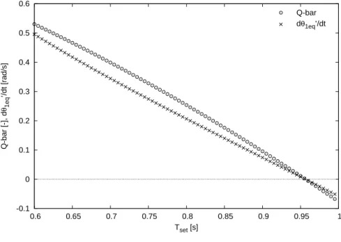
Fig. 5 plots ¯Q calculated by Eq. (32) and ˙θ′_1eq calculated by Eq. (71) with respect to Tset. Stable gait generation was impossible where Tset ≥ 1.0 [s]

because the walker could not overcome the potential barrier at mid-stance. The value of ¯R in the generated gaits was 0.968669 [-]. This is close to 1.0

and implies that the collision phase is less effective in stabilization in all the generated gaits.

From Fig. 5, we can see that both ¯Q and ˙θ′_1eq monotonically decrease as

Tsetincreases. The convergence property changes from the speed mode to the

totter mode through the deadbeat mode as expected. The deadbeat mode is represented by ¯Q = 0, and this condition is equivalent to ˙θ′_1eq = 0. We can confirm that both ¯Q and ˙θ′_1eqreach zero with the same Tset from Fig. 5.

Fig. 6 plots the evolution of the state error, ∆ ˙θ−_1(i), with respect to the number of steps where Tset = 0.80 [s]. The robot started from the condition

immediately before impact where the angular velocity is 0.1 [rad/s] smaller than the steady value, ˙θ−_1eq. With this Tset, as indicated by the result in Fig.

5, the generated gait should exhibit the speed mode ( ¯Q = 0.253726 [-]). From

Fig. 6, we can confirm that the state error monotonically converges to zero without vibrating and that the stance phases are much more effective than the collision phases in the gait stabilization.

-0.1 0 0.1 0.2 0.3 0.4 0.5 0.6 0.6 0.65 0.7 0.75 0.8 0.85 0.9 0.95 1 Q-bar [-], d θ1eq ’/dt [rad/s] T_set [s] Q-bar dθ_1eq’/dt

-0.12 -0.1 -0.08 -0.06 -0.04 -0.02 0 0.02 0 1 2 3 4 5 6

State error [rad/s]

Number of steps

Collision phase Stance phase

Immediately before impact Immediately after impact

Fig. 6 Evolution of state error where α∗= 0.20 [rad] and Tset= 0.80 [s]

Next, we analyze the convergence property where Tset= 0.99 [s]. With this Tset, the generated gait should exhibit the totter mode ( ¯Q =−0.0586365 [-]).

In this case, we also made the robot start from the same condition of Fig. 6. Fig. 7 plots the evolution of the state error with respect to the number of steps. We can confirm that the state error vibrationally converges to zero.

Finally, we examine the case where Tset = 0.9565 [s]. The result in Fig. 5

suggested that ¯Q becomes almost zero and the generated gait should exhibit

the deadbeat mode with this Tset. Fig. 8 plots the evolution of the state error

with respect to the number of steps. We can see that the convergence speed is the fastest but the deadbeat mode is not achieved in contradiction to the analysis result. This error is caused by neglecting the error terms higher than the second order in the derivation of ¯Q or by setting the initial state error to

-0.12 -0.1 -0.08 -0.06 -0.04 -0.02 0 0.02 0 1 2 3 4 5 6

State error [rad/s]

Number of steps

Collision phase Stance phase

Immediately before impact Immediately after impact

Fig. 7 Evolution of state error where α∗= 0.20 [rad] and Tset= 0.99 [s]

-0.12 -0.1 -0.08 -0.06 -0.04 -0.02 0 0.02 0 1 2 3 4 5 6

State error [rad/s]

Number of steps

Collision phase Stance phase

Immediately before impact Immediately after impact

7 Conclusion and future work

In this paper, we analyzed the stability principle underlying an underactuated compass gait with constraint on impact posture based on the linearization of motion and clarified the following properties.

– The transition function of the state error for the stance phase can be

an-alytically derived as a scalar function of the steady angular velocities by using the linearization of motion.

– The applied output following control to the desired time trajectory has the

tendency to enhance the convergence rate with the increase of Tset. – The collision phase is always stable regardless of the robot’s physical

pa-rameters and the relative hip angle.

– There is an error between the actual convergence rate and the calculated

¯

Q. This is caused by neglecting the error terms higher than second order

in the derivation of ¯Q or by setting the initial state error to a significantly

large value.

The next problem to be solved is to develop the method for setting on the deadbeat mode without the need of numerical analysis. To achieve this, the steady angular velocities, ˙θ±_1eq, must be analytically derived according to the applied output following control. There is a great deal of complexity, however, about the solution in a bipedal gait even in the case with constraint on impact posture. Now we are working on 1-DOF limit cycle walkers such as rimless wheels as the first step toward solving this problem. Classifying the type of output following control that tends to improve the convergence speed is also left as a future work. Furthermore, investigation of the case incorporating the tracking error and PD feedback control is a necessary step toward practical application.

Acknowledgements This research was partially supported by a Grant-in-Aid for Scientific

Research, (C) No. 24560542, provided by the Japan Society for the Promotion of Science (JSPS).

References

1. T. McGeer, “Passive dynamic walking,” Int. J. of Robotics Research, Vol. 9, No. 2, pp. 62–82, 1990.

2. T. McGeer, “Passive walking with knees,” Proc. of the IEEE Int. Conf. on Robotics

and Automation, Vol. 3, pp. 1640–1645, 1990.

3. A. Goswami, B. Espiau and A. Keramane, “Limit cycles in a passive compass gait biped and passivity-mimicking control laws,” Autonomous Robots, Vol. 4, Iss. 3, pp. 273–286, 1997.

4. F. Asano and Z.-W. Luo, “Energy-efficient and high-speed dynamic biped locomotion based on principle of parametric excitation,” IEEE Trans. on Robotics, Vol. 24, No. 6, pp. 1289–1301, 2008.

5. M. Vukobratovi´c and J. Stepanenko, “On the stability of anthropomorphic systems,”

6. A. Goswami, B. Thuilot and B. Espiau, “A study of the passive gait of a compass-like biped robot: symmetry and chaos,” Int. J. of Robotics Research, Vol. 17, No. 12, pp. 1282–1301, 1998.

7. J. W. Grizzle, G. Abba and F. Plestan, “Asymptotically stable walking for biped robots: Analysis via systems with impulse effects,” IEEE Trans. on Automatic Control, Vol. 46, No. 1, pp. 51–64, 2001.

8. M. J. Coleman, A. Chatterjee and A. Ruina, “Motions of a rimless spoked wheel: a simple three-dimensional system with impacts,” Dynamics and Stability of Systems, Vol.12, Iss. 3, pp.139–159, 1997.

9. F. Asano, “Stability principle underlying passive dynamic walking of rimless wheel,”

Proc. of the IEEE Int. Conf. on Control Applications, pp. 1039–1044, 2012.

10. F. Asano and Z.-W. Luo, “Asymptotically stable biped gait generation based on stability principle of rimless wheel,” Robotica, Vol. 27, Iss. 6, pp. 949–958, 2009.

11. F. Asano, “Stability analysis of passive compass gait using linearized model,” Proc. of