Numerical Inversion
of
the Laplace Transform Using a
Continuous
Euler Transformation
京都大学数理解析研究所 大浦拓哉 (Takuya Ooura)
Research Institute for Mathematical Sciences, Kyoto University
1
Introduction
The Laplace transform of function$g(t)$ is defined by
$G(s)= \int_{0}^{\infty}e^{-}gst(t)dt$ (1.1)
andits inversion is given by
$g(t)= \frac{1}{2\pi i}\int_{\gamma i\infty}^{\gamma+i}-\infty e^{i}tG(S)ds$ , $\gamma>\sigma$, (1.2)
where $\sigma$ is the abscissa of convergence for (1.1). It is known that numerical evaluation of the
integral (1.2) is difficult [2]. The integral (1.2) is a Fourier type integral:
$g(t)= \frac{e^{\gamma t}}{2\pi}\int_{-\infty}^{\infty}e^{itx}c(\gamma+ix)d_{X}$ (1.3)
with a slowly convergent integrand. Accordingly its computation accompanies a serious difficulty
[1]. Recently, the author proposed a continuous Euler transformation that accelerates the
con-vergence of the integral of such type and we showed that the continuous Euler transformation is effcient in computing the Fourier transforms ofslowlydecaying function by using FFT [5].
In this paper, we apply the continuous Euler transformation to the numerical evaluation of the integral (1.3) and propose a new method to compute numerical inversion of the Laplace transform using the continuous Euler transformation and FFT.
2
Continuous
Euler
transformation
An alternating series
$S= \sum_{n=0}^{\infty}(-1)^{n}f(n)=\sum_{n=0}^{\infty}ef(i\pi nn)$ (2.1)
is a discrete approximation to a Fourier type integral
$I= \int_{0}^{\infty}e^{i\pi}fx(x)dx$ (2.2)
with a mesh size 1. So we may expect that a continuous version of the Euler transformation, if any, will accelerate the convergenceofintegrals of Fourier type.
2.1
Definition
of the Conventional Euler Transformation
The Euler transformation truncated at the N-th term of an alternating series
$S= \sum_{=n0}^{\infty}(-1)^{n}f(n)$ (2.3)
is defined by
$s_{\mathrm{E}\mathrm{u}}^{\langle N)}= \sum_{m}^{-1}1\mathrm{e}\mathrm{r}N=0w^{(N)}m(-1)^{m}f(m)$ , $w_{m}^{\mathrm{t}^{N}}=) \sum_{+n=m1}^{N}\frac{1}{2^{N}}$ , (2.4)
where $w_{m}^{\langle N)}$
are the weights of the linear sequence transformation [7]. The weights $w_{m}^{(N)}$ happen
to be the probability of the binomial distribution.
2.2
Deflnition of the
Continuous
Euler Transformation
We define the continuous Eulertransformation for the integral
$I= \int_{0}^{\infty}e^{i\omega x}f(X)dx$
,
$\omega>0$ (2.5)by
$I_{w}^{(L)}= \int_{0}^{L}w(x;p,q)f(X)ei\omega xdX$ , $w(x;p,q)= \int_{x/\mathrm{p}q}^{\infty}-\phi(t)dt$
.
(2.6)Where $\phi(t)$ is a prescribed function $\mathrm{S}\mathrm{a}\mathrm{t}\mathrm{i}\mathrm{s}\Phi$ing
$\int_{-\infty}^{\infty}\phi(t)dt=1$ , $\lim_{tarrow\pm\infty}\phi(t)=0$ (2.7)
and$p$ and $q$ are constants depending on $L$ and $\omega$
.
2.3
Convergence of the
Continuous
Euler TRansformation
In this section, We take thefollowing$w$
$w(x;p, q)= \int_{x/p-q}^{\infty}\frac{1}{\sqrt{\pi}}e-t^{2}dt=\frac{1}{2}\mathrm{e}\mathrm{r}\mathrm{f}_{\mathrm{C}(x/-}pq)$ (2.8)
and choose $L=2pq$
.
We then have the following.Theorem 1 We assume that $f(z)$ is regular in a domain $|\arg(z+1/2)|\leq\delta$ with $0<\delta<\pi/2$,
that $|f(Z)|\leq M$ in the domain, and that
$\lim\max|f(R-1/2+iR\tan\theta)|=0$
.
$Rarrow\infty|\theta|\leq\delta$
Then, for arbitrary $\alpha$ such that $\alpha\leq\tan\delta,$ $0<\alpha<1$ we have
$|I-I_{w}(L)|<M( \frac{\sqrt{\pi}p}{\sqrt{2}\sqrt{1-\alpha^{2}}}e^{(q-}"’\alpha p/2)2/\mathrm{t}^{1-}\alpha^{2})+\frac{\sqrt{\pi}p}{4}+\frac{\sqrt{2}}{\omega\alpha}e(q-\omega\alpha p)q)e^{-q}2$ (2.9)
The proof of Theorem 1 is in $[5, 3]$
.
Now, we choose$p$ and$q$ such that $p= \frac{\sqrt{L}}{\sqrt{\omega\alpha}}$ , $q= \frac{\sqrt{\omega\alpha L}}{2}$,then theerror of the approximation is bounded as
$|I-I_{w}^{\mathrm{t}}L \rangle|<M(\frac{\sqrt{\pi L}}{\sqrt{2\omega\alpha}\sqrt{1-\alpha^{2}}}+\frac{\sqrt{\pi L}}{4\sqrt{\omega\alpha}}+\frac{\sqrt{2}}{\omega\alpha})e^{-\omega\alpha L/4}$
.
(2.11)Hence, the error of$I_{w}^{(L)}$ always decays exponentially as $Larrow\infty$
and the continuous Euler trans-formation accelerates the convergence of Fourier type integrals for$\mathrm{t}\mathrm{h}o$se $f$ described in Theorem
1.
2.4
Efflcient Weight Function
To improve the convergenceof the continuous Euler transformation, the weight function
$w(x;p,q)= \int_{x}^{\infty}/\mathrm{P}^{-}q\phi(t)dt$ (2.12)
should be taken so that
1. $|\Phi(\omega)|$ decays rapidly for large $|\omega|$
2. $|\phi(t)|$ decays rapidly for large $|t|$,
where $\Phi(\omega)$ is the Fourier transform of$\phi(t)[4]$
.
An example ofan efficient weight function is$w(x;p, q)= \frac{1}{\pi I\mathrm{o}(\beta)}\int_{/p-q}x\frac{\sinh\sqrt{\beta^{2}-t^{2}}}{\sqrt{\beta^{2}-t^{2}}}\infty dt$ (2.13)
with parameters $L=2pq,$ $q=\beta,$ $p\geq\omega^{-1}[3]$
.
The error of$I_{w}^{\{L)}$ using this weight function decays$O(e^{-L/(})2_{\mathrm{P})}$ as $Larrow\infty$
.
If we set $p=\omega^{-1}$, then the error decays $O(e^{-\omega L/2})$ and the coefficient ofthe exponent is twice as great as the coefficient of (2.11).
3
Numerical
Inversion
of the Laplace Transform
3.1
Method
using
the
Continuous Euler Transformation and FFT
We first apply the continuous Euler transformation to (1.3), and obtain
$g_{w}^{(L)}(t)= \frac{e^{\gamma t}}{2\pi}\int_{-L_{-}^{+}}^{L}W(|X|;p, q)e^{ilx}G(\gamma+ix)d_{X}$
.
(3.1) We next approximate it by the discrete summation with mesh size $h$ to obtain$g_{w}^{(N,h)}(t)= \frac{he^{\gamma t}}{2\pi}n=-\sum^{N}w+N_{-}(|nh|;p, q)eG:tnh(\gamma+inh)$, (3.2)
where $N\pm=\lfloor L_{\pm}/h\rfloor$ ($\lfloor x\rfloor$ denotes the largest integer $\leq x$).
To keep the precision of the continuous Euler transformation, we should make $p,$$q$ depend
on $L\pm \mathrm{a}\mathrm{n}\mathrm{d}\omega$
.
Here we fix the paraneters$p,$$q$ with a view to using FFT. For $L_{+}=Nh/2-h$,
$L_{-}=Nh/2$ and $t=2\pi k/(Nh),$ $(3.2)$ becomes
$g_{w}^{\langle N,h)}( \frac{2\pi k}{Nh})=\frac{he^{\gamma l}}{2\pi}\sum_{Nn=-/2}^{N/1}w(|nh|;p,q)G(\gamma 2-+inh)e^{2\pi}ink/N$, (3.3)
3.2
Error
Estimation
The approximation $g_{w}^{(N,h\rangle}$ includes thefollowing error $s$
A. Error ofthe continuous Euler transformation: $g(t)-g_{w}^{(}(tL))$
B. Error of the discrete approximation: $g_{w}^{\langle L)}(t)-g_{w}^{\mathrm{t}h}())N,t$
.
By Theorem 1, the error committed by by A is
$|g(t)-g_{w}((L)t)|< \frac{M}{\pi}(\frac{\sqrt{\pi}pe^{\mathrm{t}-}qt\alpha p/2)2/(1-\alpha^{2})}{\sqrt{2}\sqrt{1-\alpha^{2}}}+\frac{\sqrt{\pi}p}{4}+\frac{\sqrt{2}e^{\mathrm{t}q-t}p\rangle\alpha q}{t\alpha})e-q2\gamma t$, (3.4)
where $w(x;p, q)= \frac{1}{2}\mathrm{e}\mathrm{r}\mathrm{f}_{\mathrm{C}}(x/p-q)$ and $L=Nh/2=2pq$
.
The error due to$\mathrm{B}$ isan errorof the discrete Fourier transform. We can estimate thiserrorby
an extension of the theorem on the discrete Fourier transform [6, chapter 3.3] and obtain
$|g_{w}^{(L)}(t)-g_{w}((N,h)t)|< \frac{\hat{M}L}{2\pi}\mu+\frac{d_{\pm^{\hat{\epsilon}}}}{2\pi}e\gamma t\frac{ML}{2\pi}et\gamma-+q2$
(3.5)
$\mu=\frac{\exp(\gamma l-d+^{t-}2\pi d_{+/h)}}{1-\exp(-2\pi d_{+}/h\rangle}+\frac{\exp(\gamma t+d_{-}t-2\pi d_{-/h})}{1-\exp(-2\pi d_{-}/h)}$, (3.6)
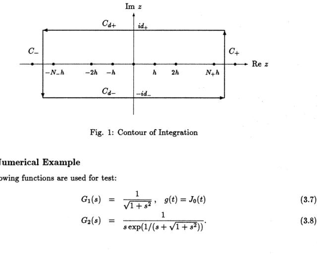
where $G(\gamma+iz)$ is regular in the $\mathrm{d}\mathrm{o}\mathrm{m}\mathrm{a}\mathrm{i}\mathrm{n}-d_{-}\leq{\rm Im} z\leq d_{+},\hat{M}$ is anupper bound of $|G(\gamma+iz)|$
in the domain, and $\hat{\epsilon}$is an upper bound of$|G(\gamma+iz)|$ on the contour ofintegration
$C_{+}$ and $\mathit{0}_{-}$
.
$\iota_{-}\sim$
Fig. 1: Contour of Integration
3.3
Numerical Example
The following functions are used for test:
$G_{1}(s)$ $=$ $\frac{1}{\sqrt{1+s^{2}}}$ , $g(t)=J_{0}(t)$ (3.7)
result using the weight function
$w_{1}(x;p,q)= \frac{1}{2}\mathrm{e}\mathrm{r}\mathrm{f}\mathrm{c}(X/p-q)$ (3.9)
is shown in Fig. 2 and theerror is shown in Fig. 3.
(a) $G(s)=\ovalbox{\tt\small REJECT}_{+\delta}^{\mathrm{J}}1$ (b) $G(s)= \frac{1}{s\exp(1/(s+\frac{1+s}{}))}$
Fig. 2: Approximations to the Inversion of the Laplace Transform: $g_{w}^{(N,h)}( \frac{2\pi k}{Nh}),$$N=512,$ $h=0.125$
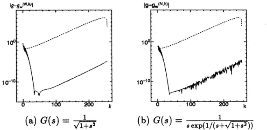
(a) $G(S)=\sqrt{1+s^{2}}^{1}$ (b) $G(s)= \frac{1}{s\exp(1/(\theta+\sqrt{1+s}))}$
Fig. 3: Absolute error of the Inversion of the Laplace Transform: $g_{w}^{(N,h)}( \frac{2\pi k}{Nh}),$ $N=512,$ $h=0.125$
We chose $N=512,$ $h=0.125,$ $\gamma=1,$ $L=Nh/2=2pq$ and computed in double precision that
has 53 bit accuracy. buncation error of the continuous Euler transformation was set to $10^{-12}$ and
the parameter $q$ is chosen so that $\exp(-q^{2})=10^{-12}$
.
The broken line in Fig. 3 denotes the errorof the direct transform that does not use $w(x;p, q)$
.
By (3.5), the error bound increases exponentially for large$t$
.
By (3.4),theerror bound becomesvery large if
$q-tp/2>0$
, i.e. $t<2q/p=3.45$.
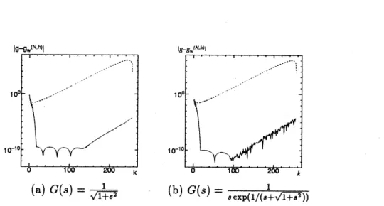
This error estimation is consistent with the numerical result.Next, we computed the sane transform using the efficient weight function
$w_{2}(x;p,q)= \frac{1}{\pi I\mathrm{o}(\beta)}\int_{x/}^{\infty}p-q\frac{\sinh\sqrt{\beta^{2}-t^{2}}}{\sqrt{\beta^{2}-t^{2}}}dt$ (3.10)
with the parameters $N=512,$ $h=0.125,$ $\gamma=1,$ $L=Nh/2=2pq$ and $e^{-\beta}=e^{-q}=10^{-13}$
.
Theerror is shown in Fig. 4.
The error of the approximation using $w_{2}(x;p, q)$ is large in$t<1.7$ that is onlyhalfthe interval
(a) $G(s)= \frac{1}{\sqrt{1+s}}$ (b) $G(s)= \frac{1}{s\exp(1/(_{\delta}+\sqrt{1+s^{2}}))}$ Fig. 4: Absolute error of the Inversion of the Laplace Transform: $g_{w}^{(N,h}() \frac{2\pi k}{Nh})$ using
$w_{2},$ $N=512$,
$h=0.125$
3.4
Execution Time
We measured the execution time on SUN Ultra SPARC-I $200\mathrm{M}\mathrm{H}\mathrm{z}$ machine with SUN Workshop
cc 4.2.1 compiler. Actual execution time is shown in Table 1. Table 1: Execution Time to Transform
The weight function we used is $w_{2}(x;p,q)$ with the same parameters as in section 3.3. We also
compared with Hosono’s method [2] with 30-point Euler transformation.
References
[1] P. J. Davis and P. Rabinowitz, Methods of Numerical Integration (Second Edition), Academic
Press, 1984.
[2] T. Hosono, Numerical Inversion of the Laplace Transform in High Precision (in Japanese),
RIMS Kokyuroku, No.422, Kyoto University, 1981.
[3] T. Ooura, Study on Numerical Integration ofFourier Type Integrals (in Japanese), Doctoral Thesis, University of Tokyo, 1997.
[4] T. Ooura, A Continuous Euler Transformationand Accelerationofthe ConvergenceofFourier
Type Integrals (in Japanese), RIMS Kokyuroku, No.1084, Kyoto University, 1999.
[5] T. Ooura, A Continuous Euler Transformation and its Application to the Fourier Transform ofa Slowly Decaying Function, J. Comput. Appl. Math., Accepted for publication, (The Same
Title, RIMS Preprint, No.1233, Kyoto University, 1999).
[6] F. Stenger, Numerical Methods Based on Sinc and Analytic Functions, Springer Verlag, 1993.