JAIST Repository: Research on the Minimum Moves of Rolling Cube Puzzles

全文

(1)JAIST Repository https://dspace.jaist.ac.jp/. Title. Research on the Minimum Moves of Rolling Cube Puzzles. Author(s). YAO, Jiawei. Citation Issue Date. 2021-03. Type. Thesis or Dissertation. Text version. author. URL. http://hdl.handle.net/10119/17159. Rights Description. Supervisor:上原隆平, 先端科学技術研究科, 修士(情報科学). Japan Advanced Institute of Science and Technology.

(2) Master’s Thesis. Research on the Minimum Moves of Rolling Cube Puzzles. Jiawei Yao. Supervisor Ryuhei Uehara. Graduate School of Advanced Science and Technology Japan Advanced Institute of Science and Technology (Information Science). March 2021.

(3) Abstract Rolling cube puzzles are a puzzle game that rolls the die which is placed on a board to complete a goal followed certain rules. A universal goal is to roll the die which is at the upper left corner of the board over all labeled cells of the board exactly once. When the die rolls over a labeled cell, the number on the top face of the die must be the same as the number of the cell on which it lies. Rolling cube puzzles have a long history. Rolling cube puzzles were popularized by Martin Gardner in his mathematical games columns, which is published in Scientific American. In 2007, Kevin Buchin et al. researched the rolling cube puzzles and proved that solving rolling cube puzzles is NPcomplete where rolling cube puzzles are defined by a six-sided die on a square grid board. However, there are several related puzzles and open problems posed in the paper by Kevin Buchin et al. In this research, we focus on one of these open problems, that is, the problem to find the minimum moves of solving rolling cube puzzles when the initial state and the final state of the die are given. In order to get some properties of this problem, we refine this problem and introduce new motions of this problem. We only discuss the situation that the initial state of the die and the final state are given and the die can be rolled freely on a board without inaccessible cells. Then, we divide this problem into two cases. One is that the die can roll along a path, whose length is equal to Manhattan distance without any detours. The other is that the die can roll in all four directions on an unlimited board. By the experiment on the first case, we found the area, that is we can roll a die to find all the possible states on a cell only along a path of length equal to Manhattan distance. We also found the optimal number of the minimum moves to find all the possible states on a cell in the other area. According to these results of the experiments, we give an algorithm for finding a general solution for the problem and analysis the complexity of this algorithm. In the algorithm, we divide the problem into four subproblems. The first one asks whether the path from the initial state to the final state exists or not. The second one asks if a die can reach to all the final states from the initial state along a path of length equal to the Manhattan distance or not. Thirdly, the algorithm determines if a die can reach the final state with a detour of length not greater than 2 addition to its Manhattan distance. The complexity of this part will take O(4d(T ) ) time, where d(T ) is the depth of the BFS tree T, because we need to explore the four moving directions.

(4) of the die. However, we know the upper bound of the maximum steps of a detour to find all the possible states on a cell. That means we only need to explore the area along the paths of the length of the Manhattan distance with the maximum detour. Furthermore, if the algorithm records all the states of the die after it has rolled and the cell of these states, the running time is drastically reduced in the manner of dynamic programming. Meanwhile, we verify that the new state does not duplicate in the table. After these 2 optimizations, the complexity of this part will be reduced to O(Dm × d(T )) time, where Dm is the Manhattan distance between the initial cell and the goal cell. Finally, we only have the situation left, that is the minimum moves are equal to Manhattan distance plus 4. For this last subproblem, we transform the goal to find the corresponding state on the cell next to the initial cell. Follow these steps, we can get a general solution to find a shortest path between the starting point and the ending point when the initial state of the die and the final state are given and the die can be rolled freely on a board without inaccessible cells.. 2.

(5) Contents 1 Introduction 1.1 Background . . . . . . . . . . . . . . . . . . . . . . . . . . . . 1.2 Research Purposes . . . . . . . . . . . . . . . . . . . . . . . . 1.3 Composition . . . . . . . . . . . . . . . . . . . . . . . . . . . .. 1 1 2 3. 2 Preliminaries 2.1 Definition of Rolling Cube Puzzles . . . . . . . . . . . . . . 2.1.1 General Rolling Cube Puzzles . . . . . . . . . . . . . 2.1.2 State of a Die . . . . . . . . . . . . . . . . . . . . . . 2.1.3 Four Moving Directions of a Die, East, South, West, North . . . . . . . . . . . . . . . . . . . . . . . . . . 2.2 Parity Property . . . . . . . . . . . . . . . . . . . . . . . . . 2.3 Complexity of the Puzzle with only one Block . . . . . . . .. . . .. 4 4 4 6. . . .. 6 7 8. 3 Analysis of the Rolling Cube Puzzle 9 3.1 Some Definitions of Rolling Cube Puzzle . . . . . . . . . . . . 9 3.1.1 The Definition of Dm ((x, y), (x′ , y ′ )) . . . . . . . . . . . 9 3.1.2 The Definition of Path P and Lp (P ) . . . . . . . . . . 9 3.1.3 The Definition of Ld (P ) . . . . . . . . . . . . . . . . . 10 3.1.4 The Definition of k(P, U BL) and Kf inal (((x, y), U BL), (x′ , y ′ )) 10 3.1.5 Parity of Ld . . . . . . . . . . . . . . . . . . . . . . . . 10 3.1.6 The Definition of Lud (((x, y), U BL), ((x′ , y ′ ), U ′ B ′ L′ )) . 11 3.2 Rolling a Die along a Path of Length Lp = Dm . . . . . . . . . 12 3.2.1 Preparation . . . . . . . . . . . . . . . . . . . . . . . . 12 3.2.2 Some Simple Properties . . . . . . . . . . . . . . . . . 12 3.2.3 2 Parts of a Path to a Red Cell . . . . . . . . . . . . . 13 3.3 Minimum Number of Rolling a Die on an Unlimited Board . . 14 3.3.1 Preparation . . . . . . . . . . . . . . . . . . . . . . . . 14 3.3.2 The Results on an Unlimited Board . . . . . . . . . . . 14 3.3.3 The Cell whose Lud is 6 . . . . . . . . . . . . . . . . . . 15 3.3.4 A General Transformation . . . . . . . . . . . . . . . . 15 1.

(6) 3.3.5 3.3.6 3.3.7 3.3.8. Efficient algorithm for reachability problem . Cells whose Lud is 4 . . . . . . . . . . . . . . A Transformation when Ld = 4 . . . . . . . Cells whose Lud is 2 . . . . . . . . . . . . . .. 4 Implementation and Analysis of the Algorithm 4.1 Efficient algorithm for reachability . . . . . . . . 4.2 Function IFK() . . . . . . . . . . . . . . . . . . 4.3 Function IFYC() . . . . . . . . . . . . . . . . . 4.4 4 Functions East(), South(), West(), North() . . 4.5 Function EXP() . . . . . . . . . . . . . . . . . . 4.6 Complexity of Function EXP() . . . . . . . . . 4.7 Function TRTSC() . . . . . . . . . . . . . . . . 4.8 Function RCP() . . . . . . . . . . . . . . . . . . 4.9 Proof of Theorem 6 . . . . . . . . . . . . . . . .. . . . . . . . . .. . . . . . . . . .. . . . .. . . . . . . . . .. . . . .. . . . . . . . . .. . . . .. . . . . . . . . .. . . . .. . . . . . . . . .. . . . .. . . . . . . . . .. . . . .. 15 16 17 17. . . . . . . . . .. 19 19 19 20 21 21 21 22 23 23. 5 Conclusion and Future Work 25 5.1 Conclusion . . . . . . . . . . . . . . . . . . . . . . . . . . . . . 25 5.2 Future Work . . . . . . . . . . . . . . . . . . . . . . . . . . . . 25.

(7) List of Figures 1.1 1.2 1.3 2.1 2.2 2.3 2.4 2.5 2.6 2.7. Rolling cube puzzles posed by Joseph O’ Rourke at CCCG 2005[3] . . . . . . . . . . . . . . . . . . . . . . . . . . . . . . . Rolling cube puzzles posed by Martin Demaine at CCCG 2005[3] An example of rolling cube puzzles when the initial state and the final state of the die are given . . . . . . . . . . . . . . . .. 3. A standard die . . . . . . . . . . . . . . . . . . . . . . . . . . Net of a standard die[6] . . . . . . . . . . . . . . . . . . . . . The two standard dice[1] . . . . . . . . . . . . . . . . . . . . . One solution of Figure 1.1[3] . . . . . . . . . . . . . . . . . . . State of a die . . . . . . . . . . . . . . . . . . . . . . . . . . . A die and a board with 2-colored corners[1] . . . . . . . . . . . Checker board pattern of alternating black and white squares. 4 5 5 6 6 7 7. 3.1 A broad . . . . . . . . . . . . . . . . . . . . . . . . . . . . . 3.2 Two ways from A to B . . . . . . . . . . . . . . . . . . . . . 3.3 Two paths of rolling a die from (0, 0, 362) to (0, 0, 241) . . 3.4 Board without blocked cells . . . . . . . . . . . . . . . . . . 3.5 Number of results without duplicated of only two directions 3.6 Lud to get the maximum possible outcomes K or K ′ on a cell 3.7 3 kinds of rolling from (0,0) to (0,0) . . . . . . . . . . . . . . 3.8 A part of Figure 3.6 . . . . . . . . . . . . . . . . . . . . . . 4.1. An example of the application of dynamic programming. . . . . . . . .. 1 2. 10 10 11 12 13 14 15 17. . . . 23.

(8) List of Tables.

(9) Chapter 1 Introduction 1.1. Background. Rolling cube puzzles are a puzzle game that rolls the die which is placed on a board to complete a goal followed certain rules. For example, Figure 1.1 is a simple rolling cube puzzle posed by Erik D. Demaine and Joseph O’ Rourke at CCCG 2005. In this puzzle, the objective is to roll the die which is at the upper left corner of the board over all labeled cells of the board exactly once. When the die rolls over a labeled cell, the number on the top face of the die must be the same as the number of the cell which it lies on. In addition to labeled cells, there are some cells called free cells which are white without any marks. The die can enter and exit these cells freely. That means the die may roll on free cells multiple times, and there is no limit to the number of the top face. Also, according to some other rules, we can get the other kinds of rolling cube puzzles as in Figure 1.2.. Figure 1.1: Rolling cube puzzles posed by Joseph O’ Rourke at CCCG 2005[3] Rolling cube puzzles have been investigated with a long history. They were popularized by Martin Gardner[1]. Over the past 20 years, considerable attention has been paid to rolling cube puzzles. In 2007, Kevin Buchin et al. 1.

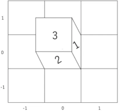
(10) Figure 1.2: Rolling cube puzzles posed by Martin Demaine at CCCG 2005[3] researched the rolling cube puzzles. In [1], they proved that solving rolling cube puzzles is NP-complete in the circumstance that rolling cube puzzles defined by a six-sided die on a square grid board. In 2011, Kevin Buchin and Maike Buchin extended their proof for rolling cube puzzles to show the complexity of rolling block maze puzzles[4]. In the same year, rolling cube puzzles were generalized by Akihiro Uejima and Takahiro Okada. They discussed the computational complexity of an expansion problem on rolling cube puzzles and substantiated the generalized problem is NP-complete when using different kinds of board such as a triangular grid board or when using some other types of dice such as eight-sided and twenty-sided die[2]. However, there are several related puzzles and open problems posed in the paper by Kevin Buchin et al. As can be seen, it still requires further research how to resolve these problems.. 1.2. Research Purposes. In this research, we focus on one of these open problems, that is, the problem to find the minimum moves of solving rolling cube puzzles when the initial state and the final state of the die are given. In this problem, we know the coordinate of the initial cell is (x, y) and the coordinate of the final cell is (x′ , y ′ ). We also know the initial state of the die is k and the final state is k ′ . These states are dependent on the location relations of different faces of a die when it lies on the initial cell or the final cell. For these given conditions, we are devoted to find a shortest path to reach the final state k ′ from the initial state k by only one die when the die can be rolled freely on a board without inaccessible cells. Figure 1.3 is an example of rolling cube puzzles when the initial state and the final state of the die are given. Specifically, we discuss the details of the moves and procedures for solving rolling cube puzzles and make the processes explicit when the initial state and final state of the die are given. Based on this, we give an algorithm for finding a general solution for the problem and analysis the complexity of this algorithm.. 2.

(11) Figure 1.3: An example of rolling cube puzzles when the initial state and the final state of the die are given Rolling cube puzzles are a special puzzle with extraordinary properties which are critically different from other conventional puzzles. Rolling cube puzzles require a three-dimensional way of thinking, because of not only the complexity of the board but also using a die. Elucidation of these properties provides a new and useful perspective on the characterization of complexity classes. There is no doubt that solutions to rolling cube puzzles will unlock the critical bottleneck of solving the other problem with the same nature of rolling cube puzzles.. 1.3. Composition. In Chapter 2, we use a simple puzzle (Figure 1.1) to show the basic properties and characteristics of rolling cube puzzles. For instance, the state of a die and the parity property of rolling cube puzzles will be introduced. In addition, we explain a part of the proof about the complexity of rolling block maze puzzles with only one block[4]. In Chapter 3, we analyze rolling cube puzzles without inaccessible cells when the initial state of the die and the final state are given. In Chapter 4, we show an algorithm for finding a shortest path to solve our problem and analysis the complexity of this algorithm.. 3.

(12) Chapter 2 Preliminaries In this chapter, we introduce the basic definition of the rolling cube puzzles in Section 2.1. In Section 2.2, we illustrate some basic properties which are central to solving the problem investigated in Chapter 3.. 2.1 2.1.1. Definition of Rolling Cube Puzzles General Rolling Cube Puzzles. In general, a rolling cube puzzle is composed by one or more dice, a board, a goal, and some rules. In this research, we restrict ourselves to puzzles with one die. There are many kinds of dice, here we use the standard die, which is more common. A standard die is accounted as a cube with six faces labeled one to six and the sum of the two numbers labeled on opposite faces is always seven (Figure 2.1). and Figure 2.2 is a geometry net of this standard die.. Figure 2.1: A standard die There are two kinds of the standard dice. According to how the number on the labeled faces are arranged, they can be classified as right-handed or left-handed dice. In particular, in the case, that is, the numbers from 1 to 3 are arranged counterclockwise when we gaze the vertex in the center of 4.

(13) Figure 2.2: Net of a standard die[6] the faces labeled by 1, 2, and 3, the die is called right-handed die. On the contrary, when they are lined clockwise, the die is left-handed die. Figure 2.3 is an illustration.. Figure 2.3: The two standard dice[1] The board is a grid with three types of cells: labeled cells, free cells and blocked cells. As we introduced at the beginning of this paper, labeled cells must be accessed exactly once when the number on the top face of the die should be the same as the label of the cell it lies on. Free cells can be visited with no limit. That means a die can visit free cells with any number on the top face and any times. Then, definition of blocked cells is simple. No matter what happens, the die cannot visit blocked cells. Given a board, we need to roll the die on the board to complete some missions. See Figure 1.1. It is a puzzle that the die must visit all the labeled cells. One solution of Figure 1.1 is ESENEESSWWWWN, where E,S,W,N mean East, South, West, and North, respectively (Figure 2.4). In other cases, we may be given a initial state and a final state of the die (Figure 1.3). We consider the case when the initial state and the final state of the die are determined.. 5.

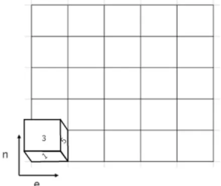
(14) Figure 2.4: One solution of Figure 1.1[3]. 2.1.2. State of a Die. We defined the state of a die by a label U BL, where U is the label on the top of the die, B the label on the back face and L the label on the left face. For example, in Figure 2.5, the state of this die is 356 (2 is the label on the front face).. Figure 2.5: State of a die. 2.1.3. Four Moving Directions of a Die, East, South, West, North. At last, we define that the four moving directions of a die is East, South, West and North in the coordinate system, for the cell(x, y) the die lied on is given. After an East move, the cell the die lied on will change from (x, y) to (x + 1, y). After a South move, the cell the die lied on will change from (x, y) to (x, y − 1). After a West move, the cell the die lied on will change from (x, y) to (x − 1, y). After a North move, the cell the die lied on will change from (x, y) to (x, y + 1). The state of a die also change after a move which is dependent by the kind of the die. 6.

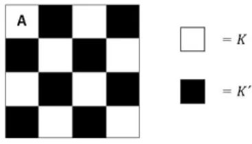
(15) 2.2. Parity Property. Generally, all vertices of the state graph can be divided into two sets of the same size with no edges between the two vertices in the same set. By symmetry, we only need to discuss two of the four orientations if the initial state is given. In other word, assume we color the corners of the die alternatively with white and black (Figure 2.6(a)), and roll this die over all cells of a board. All nodes of the board will be dyed in these two colors like it shows in Figure 2.6(b). Only two orientations are allowed in a labeled cell because it is not possible to turn the die 90 degrees in the horizontal direction.. Figure 2.6: A die and a board with 2-colored corners[1] Now, we have a piece of checker board pattern of alternating black and white squares like Figure 2.7. Then, we define that K is a set of the all states of a die at a white cell in Figure 2.7. K ′ is a set of the all states of a die at a black cell. For example, if a die starts with (362) at board A. Then K is {(362), (315), (124), (153), (241), (236), (465), (412), (546), (531), (654), (623)} and K ′ is {(132), (145), (213), (264), (321), (356), (451), (426), (514), (563), (635), (642)}. The cardinality of K and K ′ are 12.. Figure 2.7: Checker board pattern of alternating black and white squares. 7.

(16) 2.3. Complexity of the Puzzle with only one Block. Rolling block mazes puzzle with only one block can be solved using linear time and space[4]. Kevin Buchin and Maike Buchin consider that if one of the position results from the previous position of it, the size of the state graph is determined by the size of the board, independent of the size of the block. Then, the puzzle can be solved by searching the state graph for a path from the starting to the ending position. Thus, if using breadth first search to solve this, it can be done in time linear in the number of edges.. 8.

(17) Chapter 3 Analysis of the Rolling Cube Puzzle In this chapter, we reveal some properties drawn quickly of the case. In Section 3.1, we define some notions and notations that we will use later. In Section 3.2, we discuss a simple case that we know a starting position and an ending position of the die. Further, we analyze the case rolling a die on a board without any limits in Section 3.3.. 3.1 3.1.1. Some Definitions of Rolling Cube Puzzle The Definition of Dm ((x, y), (x′ , y ′ )). First of all, we define that Dm ((x, y), (x′ , y ′ )) is |x − x′ | + |y–y ′ |, when the coordinate of the start point is (x, y), and coordinate of the end point is (x′ , y ′ ). Dm is “manhattan distance”. For example, Dm ((0, 0), (3, 2)) = 3 + 2 = 5.. 3.1.2. The Definition of Path P and Lp (P ). We define that path P is the route from (x0 , y0 ) to (xn , yn ) in which a die is rolling. Path P is a sequence of all the cells which the die has been visited. Path P = ((x0 , y0 ), (x1 , y1 ), ... , (xn , yn )), where Dm ((xi , yi ), (xi+1 , yi+1 )) = 1. The length Lp (P ) of a path P is |n − 1|, where n is the number of points in the path P . If we roll a die from A to B in Figure 3.1, the path α (A, B) is ((0, 0), (1, 0)). In the case, Lp (α) is 1. While we roll a die from A to C via B, the path β (A, C) will be ((0, 0), (1, 0), (2, 0)), Lp (β) is 2.. 9.

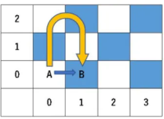
(18) In Figure 3.2, it shows us two ways to roll a die from A to B. If we roll a die along the blue arrow, the path a (A, B) is ((0, 0), (1, 0)), and Lp (a) is 1. If we roll a die along the yellow arrow, the path b (A, B) is ((0, 0), (0, 1), (0, 2), (1, 2), (1, 1), (1, 0)), and Lp (b) is 5.. Figure 3.1: A broad. 3.1.3. The Definition of Ld (P ). We define that Ld (P ) is |Lp (P )−Dm ((x0 , y0 ), (xn , yn ))|. Ld means the length of a detour. In Figure 3.2, Dm from A to B is 1. If we roll a die along the yellow arrow, Lp > Dm . That means we take a detour from A to B. For example, in this case, Ld of rolling along the yellow arrow is 4.. Figure 3.2: Two ways from A to B. 3.1.4. The Definition of k(P, U BL) and Kf inal (((x, y), U BL), (x′ , y ′ )). Now, we define that k(P, U BL) is the current state after rolling a die along the path P from the initial state U BL and Kf inal ((x, y), U BL, (x′ , y ′ )) is all the current states of one cell after rolling. That means k(P, U BL) ∈ Kf inal ((x, y), U BL, (x′ , y ′ )). Kf inal ((x, y), U BL, (x′ , y ′ )) ⊆ K or K ′ .. 3.1.5. Parity of Ld. Theorem 1 Ld is even. 10.

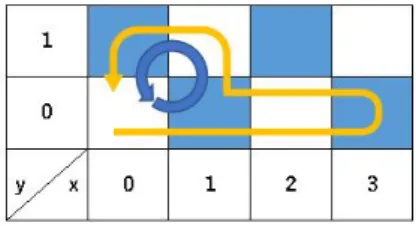
(19) Proof. According to parity in Section 2.2, when Lp = 0, k is the initial state of the die, k ∈ Kf inal ⊆ K. Meanwhile, every time Lp add one, which set of all the current states of one cell after rolling Kf inal is included in, will transform from K to K ′ or from K ′ to K. Assume Ld is odd, then Lp = Dm + odd. So, when Dm is odd, Lp is even, Kf inal ⊆ K. When Dm is even, Lp is odd, Kf inal ⊆ K ′ . But, when Lp = Dm is odd, Kf inal ⊆ K ′ . When Lp = Dm is even, Kf inal ⊆ K. Whether Dm is odd or even, the results are inconsistent. That means the assumption, Ld is odd, is false. So, Ld is even. 2. 3.1.6. The Definition of Lud (((x, y), U BL), ((x′ , y ′ ), U ′ B ′ L′ )). Before discussing the results of the experiment, we import a new notion that Lud (((x, y), U BL), ((x′ , y ′ ), U ′ B ′ L′ )) is the upper limit of the minimum of detours for one state of a die on a cell. Now, there is a problem to roll a die from a initial state (0, 0, 362) to an final state (0, 0, 241). Figure 3.3 shows us two ways to clear this problem. In Figure 3.3, the path of rolling along the blue arrow are ((0,0), (1,0), (1,1), (0,1), (0,0)). The path of rolling along the yellow arrow are ((0,0), (1,0), (2,0), (3,0), (2,0), (1,0), (1,1), (0,1), (0,0)). Ld of rolling along the blue arrow is 4 and Ld of rolling along the yellow arrow is 8. By experiment, rolling along the blue arrow is the minimum detour we need for rolling a die from (0, 0, 362) to (0, 0, 241). That means if we roll a die along the yellow arrow, we take a meaningless detour. So, we can say Lud of rolling a die from (0, 0, 362) to (0, 0, 241) is 4.. Figure 3.3: Two paths of rolling a die from (0, 0, 362) to (0, 0, 241). 11.

(20) 3.2 3.2.1. Rolling a Die along a Path of Length Lp = Dm Preparation. As mentioned above, our objective is to accomplish the case when the initial state and the final state of the die are determined. It is easy if there is no limit of steps to accomplish the case. Thus we devote to finding the minimum steps to finish this case. Now we prepare a board without blocked cells and a left-handed die. We use bearing to named movement of a die like N(north) means moving upwards (Figure 3.4).. Figure 3.4: Board without blocked cells. 3.2.2. Some Simple Properties. Due to our goal, we limit the directions of movement in only North and East. That means we roll a die in such a case Lp = Dm . So, the results we found must be the shortest paths. See Figure 3.5 for an example. In Figure 3.5, all kinds of cell (4,4), cell (3,6) and cell (6,3) is 12 without duplicate results. As we know in Section 2.2, 12 is the maximumimum possible outcomes on one cell. So, if a cell α(x1 , y1 ) is farther than cell (4,4), cell (3,6) and cell (6,3), we can find the maximumimum possible outcomes K or K ′ on the α. x1 and y1 subject to the following conditions,   |x1 | ∈ [4, +∞) ∧ |y1 | ∈ [4, +∞) |x1 | ∈ [3, +∞) ∧ |y1 | ∈ [6, +∞)  |x1 | ∈ [6, +∞) ∧ |y1 | ∈ [3, +∞) As we know in the case of Figure 1.3, it is not always can find a result in the condition whose Lp = Dm . Go a step further, if we cannot find all the 12.

(21) Figure 3.5: Number of results without duplicated of only two directions possible outcomes on a cell. That means we have to make a detour to find the remained results on this cell. For example, in Figure 3.5, the red cells are the cell α which have discussed above. That means we can find the maximumimum possible outcomes K or K ′ in the red cells by Dm . The yellow cells are a part of the cells which we cannot find the maximumimum possible outcomes by Dm . If we roll a die from a red cell, which is next to a yellow cell, to the yellow cell. Then, we can get all the possible outcomes in this yellow cell by taking a detour.. 3.2.3. 2 Parts of a Path to a Red Cell. Theorem 2 When (x, y) meet each following condition,   |x| ∈ [4, +∞) ∧ |y| ∈ [4, +∞) |x| ∈ [3, +∞) ∧ |y| ∈ [6, +∞)  |x| ∈ [6, +∞) ∧ |y| ∈ [3, +∞) we can find the maximumimum possible outcomes K or K ′ on (x, y), where Ld = 0. Proof. According to mathematical induction of the results of only two directions (Figure 3.5), we can say following. For any given a shortest path from (0, 0) to (x, y), we can find a way to transform the path into two parts. The first part is a path A from (0, 0) to (±4, ±4), (±3, ±6) or (±6, ±3). The second part is a path B from the final cell of the path A to (x, y). If we connect A and B, we also can reach the final state of the die from the initial state and keep Lp the same. 13.

(22) 2. Thus, Theorem 2 can be proved.. 3.3 3.3.1. Minimum Number of Rolling a Die on an Unlimited Board Preparation. In this step, we hope to know the range of detours. As mentioned above, we only decide the state on the start position in the case we do in this section. There is no any more limit of this case. Now we prepare a board without blocked cells and a left-handed die. Then we roll a die from (0,0) under the state of the die is 362.. 3.3.2. The Results on an Unlimited Board. Next, we talk about the results of our experiment. In this experiment, we have explored all the rolling paths in a area. In this area, the coordinate of the all cells must meet the conditions that x ∈ [−9, 9] ∧ y ∈ [−9, 9]. By this experiment, we can know all Lud of getting the maximumimum possible outcomes K or K ′ on a cell . Figure 3.6 is a path of our results. In Figure 3.6 we know Lud of blue cell is 6. Lud of orange cell is 4. Lud of green cell is 2. Lud of yellow cell is 0.. Figure 3.6: Lud to get the maximum possible outcomes K or K ′ on a cell. 14.

(23) 3.3.3. The Cell whose Lud is 6. According to the result above, cell(0,0) is one and the only one cell whose Lud is 6. If we roll a die starting from (0,0), we want to finish this rolling at (0,0). We can take 3 kinds of rolling in Figure 3.7. (a) is rolling a die along a clockwise path of length 4. For example, a path which is ((0,0), (1,0), (1,-1), (0,-1), (0,0)) is a clockwise path. By experiment, we can know that if we roll a die through (a) kind of rolling, we can find 4 kinds of outcomes {(236), (153), (546), (654)} on (0,0). Through (b) kind of rolling which is rolling a die along an anti-clockwise path of length 4, we can get the other 4 kinds of outcomes {(241), (124), (531), (623)} on (0,0). So, if we want to get the last 3 kinds outcomes {(315), (465), (412)} on (0,0), we should roll a die through (c) kind of rolling whose Ld is 6. That means we can find the maximumimum possible outcomes K on (0,0) through rolling a die along a path P , where Lp (P ) ≤ 6.. Figure 3.7: 3 kinds of rolling from (0,0) to (0,0). 3.3.4. A General Transformation. Theorem 3 For any given (x, y), (x′ , y ′ ), initial state k and final state k ′ , we can find a way to transform from the initial state k to the final state k ′ by rolling along a path P , where Lp (P ) ≤ Dm ((x, y), (x′ , y ′ )) + 6. Proof. Because we know that we can find the maximumimum possible outcomes K on the initial cell (x, y) through rolling a die along a path P , where Lp (P ) ≤ 6. We can find a way to transform from the initial state k to the corresponding state kc we need on the cell(x, y). Then, we transform from the corresponding state kc to the final state k ′ on the cell(x′ , y ′ ) by rolling along a path P ′ , where Lp (P ′ ) = Dm ((x, y), (x′ , y ′ )). Thus, Theorem 3 can be proved. 2. 3.3.5. Efficient algorithm for reachability problem. Theorem 4 For any given (x, y), (x′ , y ′ ), initial state k ∈ K, we have the following. 15.

(24) Case 1 Dm ((x, y), (x′ , y ′ )) is odd. • For any path P between (x, y), (x′ , y ′ ), the final state k ′ by P belongs to K ′ . • For any k ′ ∈ K ′ , we have some path P such that the final state by P is k ′ . Case 2 Dm ((x, y), (x′ , y ′ )) is even. • For any path P between (x, y), (x′ , y ′ ), the final state k ′ by P belongs to K. • For any k ′ ∈ K, we have some path P such that the final state by P is k′. Proof. According to parity in Section 2.2 and Theorem 3, Theorem 4 can be proved by mathematical induction. 2. 3.3.6. Cells whose Lud is 4. According to the results in Figure 3.6, Lud of β(x2 , y2 ) is 4, where x2 and y2 subject to the following conditions,   |x2 | ∈ (0, +∞) ∧ y2 = 0 |y2 | ∈ (0, +∞) ∧ x2 = 0  |x2 | + |y2 | ∈ (0, 4] . As we know in the last subsection, (0,0) is the only cell whose Lud is 6. Now, we discuss the upper limit of the area of the orange cells. In Figure 3.8, the cells on the line a satisfy to the conditions that |x2 | + |y2 | = 5. The least that can be concluded from the result above is that we can find the maximumimum possible outcomes K ′ at cell (4,1), (3,2), (2,3), (1,4) when Lp = 7. We cannot find the maximumimum possible outcomes K ′ at cell (5,0), (0,5) when Lp = 7. Due to parity property, we will never find the maximumimum possible outcomes K ′ at cell (5,0), (0,5) when Lp = 8. According to the results of our experiment, we can find the maximumimum possible outcomes K ′ at cell (5,0), (0,5) when Lp = 9. In the same way, we can find the maximumimum possible outcomes K at cell (5,1), (4,2), (3,3), (2,4), (1,5) when Lp = 8. We can find the maximumimum possible outcomes K at cell (6,0), (0,6) when Lp = 10. In this fashion, we go on discussing the cell whose Dm = 7, 8, 9. We always get the same conclusion that Lp (x = 0 ∨ y = 0 ∧ Dm = 7, 8, 9) > Lp (x ̸= 0 ∧ y ̸= 0 ∧ Dm = 7, 8, 9). 16.

(25) It is unable to roll a die to the cell(x, y), which subjects to the conditions that |x| ∈ (0, +∞) ∧ y = 0 or the conditions that |y| ∈ (0, +∞) ∧ x = 0, by a shorter path whose Ld < 4. So, we can say the upper limit of the area of the orange cells is |x| + |y| = 4 ∨ |x| ≥ 5(when y = 0) ∨ |y| ≥ 5(when x = 0).. Figure 3.8: A part of Figure 3.6. 3.3.7. A Transformation when Ld = 4. Theorem 5 For any given (x, y), (x′ , y ′ ), initial state k, final state k ′ and a path P from (x, y) to (x′ , y ′ ) satisfying the condition Ld (P ) = 4, there exists a way that we can transform the goal to find the corresponding state kc on the cell next to the initial cell(x, y) and keep Lp the same. Proof. By experiment, we know that we can find the all possible outcomes K ′ on the cell (xn , y) or the cell (x, yn ) though rolling a die along a path P from the initial cell(x, y) to (xn , y) or (x, yn ), where |xn − x| = |yn − y| = 1 and Lp (P ) = 5. Therefore, Theorem 5 can be proved by mathematical induction. 2. 3.3.8. Cells whose Lud is 2. According to the results in Figure 3.6, Ldu of γ(x3 , y3 ) is 2, where x3 and y3 subject to the following conditions,   |x3 | ∈ [1, 2] ∧ |y3 | ∈ (4, +∞) |y3 | ∈ [1, 2] ∧ |x3 | ∈ (4, +∞)  |x3 | + |y3 | ∈ [5, 8] ∧ (x3 , y3 ) ̸= (4, 4) ∧ |x3 | ∈ (0, +∞) ∧ |y3 | ∈ (0, +∞) . In the same way, we can discuss the upper limit of the area of the green cells. In the same fashion we used in the last subsection, we can know, when Lp = 8, we can find the maximumimum possible outcomes K at cell (4,4). 17.

(26) We cannot find the maximumimum possible outcomes K at cell (7,1), (6,2), (5,3), (3,5), (2,6), (1,7) when Lp = 8 we can find K at these cells when Lp = 10. Also, when Lp = 9, we can find the maximumimum possible outcomes K ′ at cell (6,3), (3,6). We can find K ′ at cell (8,1), (7,2), (2,7), (1,8) when Lp = 11. It is unable to roll a die to the cell(±4, ±3), (±5, ±3), (±3, ±4), (±3, ±5), (x, y), which subjects to the conditions that |x| ∈ [6, +∞) ∧ y = 2 or the conditions that |y| ∈ [6, +∞) ∧ x = 2, by a shorter path whose Ld < 2. Thus, we can say the upper limit of the area of the green cells is |x| ≥ 6(when |y| = 2)∨|y| ≥ 6(when |x| = 2)∨(x, y) ∈ {(±4, ±3), (±5, ±3), (±3, ±4), (±3, ±5)}.. 18.

(27) Chapter 4 Implementation and Analysis of the Algorithm 4.1. Efficient algorithm for reachability. Theorem 6 For any given (x, y), (x′ , y ′ ), initial state k and final state k ′ , we can find a shortest path from k to k ′ in O((Dm )2 × (Dm + Ld )) time. We will prove Theorem Theorem 6 in the next subsections.. 4.2. Function IFK(). According to Theorem 4, we can define a function IFK() to decide whether the goal can be achieved, when we input the state of starting point and the state of ending point. The pseudo-code of IFK() is Algorithm 1. As we know in Section 2.2, we can get the set of the maximumimum possible outcomes K or K ′ in all cells, when we know the state of starting point. We can calculate Dm from starting point to ending point, and decide whether the possible outcomes at the ending point is belonged K or K ′ . Now, we know the state of starting point is (0, 0, 362), and three states of ending point(Uk Bk Lk ). Because of parity property, if Dm is odd, the possible outcomes(Up Bp Lp ) at the ending point will belong to the set K ′ . If Dm is even, (Up Bp Lp ) will belong to the set K. Thus, when Dm is an odd, if (Uk Bk Lk ) is belong to K ′ . Then, we can say this case can be cleared. Otherwise, this case can’t be cleared. Similarly, when Dm is an even, if (Uk Bk Lk ) is belong to K. Then, we can say the input is feasible. Otherwise, this input is not feasible.. 19.

(28) Algorithm 1 Function IFK((x1 , y1 , U1 B1 L1 ), (x2 , y2 , U2 B2 L2 )) input: the state of starting point, the state of ending point output: true or false 1: if Dm is odd then 2: if (U2 B2 L2 ) ∈ K ′ then 3: return true 4: else 5: return false 6: end if 7: else if Dm is even then 8: if (U2 B2 L2 ) ∈ K then 9: return true 10: else 11: return false 12: end if 13: end if. Algorithm 2 Function IFYC(x2 , y2 ) input: the coordinate of ending point output: true or false 1: if |x2 | ∈ [4, +∞) ∧ |y2 | ∈ [4, +∞) then 2: return true 3: else if |x2 | ∈ [3, +∞) ∧ |y2 | ∈ [6, +∞) then 4: return true 5: else if |x2 | ∈ [6, +∞) ∧ |y2 | ∈ [3, +∞) then 6: return true 7: else 8: return false 9: end if. 4.3. Function IFYC(). IFYC() decides whether the cell of our goal is a cell of the yellow cells we knew in Chapter 3 or not, when we input the coordinate of ending point. IFYC() also transforms the goal to find the corresponding state on the cell (4, 4), (3, 6), (6, 3). The pseudo-code of IFYC() is Algorithm 2. 20.

(29) Algorithm 3 Function East(x1 , y1 , U1 B1 L1 , path1 ) input: the state of starting point, the path to initial state output: the state of ending point, the path to the final state 1: x2 ← x1 + 1 2: y2 ← y1 3: U2 ← L1 4: B2 ← B1 5: L2 ← 7 − U1 6: path2 ← path1 .append(x2 , y2 ) 7: return (x2 , y2 , U2 B2 L2 , path2 ). 4.4. 4 Functions East(), South(), West(), North(). East(), South(), West(), North() are four functions used to indicate the change of a die in four directions, when Lp = 1, if we input the state of starting point. For example, the pseudo-code of East() is Algorithm 3.. 4.5. Function EXP(). EXP() is a function used to decide whether the goal can be achieved by Dm + Ld , and give a path to achieve this goal. According to BFS[5], an example of the pseudo-code of EXP() is Algorithm 4.. 4.6. Complexity of Function EXP(). The complexity of this part will take O(4Dm +Ld ) time in a naive implementation, because we need to explore the four moving directions of the die. However, we know the upper bound of the maximumimum moves of a detour to find all the possible states on a cell. That means we only need to explore the area along the paths of the length of the Manhattan distance with the maximumimum detour. Furthermore, if the algorithm records all the states of the die after it has rolled and the cell of these states, the running time is drastically reduced in the manner of dynamic programming[5]. Meanwhile, we verify that the new state does not duplicate in the table. Figure 4.1 is an example of the application of dynamic programming. We can blacken the cell when a state on the cell is appeared. When we reach. 21.

(30) Algorithm 4 Function EXP((x1 , y1 , U1 B1 L1 ), (x2 , y2 , U2 B2 L2 ), Ld ) input: the state of starting point, the state of ending point, Ld output: a path to the state of ending point, or false 1: p ← (x1 , y1 ) 2: S ← (U1 B1 L1 ) 3: pf ← (x2 , y2 ) 4: Sf ← (U2 B2 L2 ) 5: Q.push(p, S, path, Dm + Ld ) 6: while Q is not an empty list do 7: p, S, path, n ← Q.pop() 8: if n ≤ 0 then 9: return false, 10: end if 11: p1 , S1 , path1 ← East(p, S, path) 12: p2 , S2 , path2 ← South(p, S, path) 13: p3 , S3 , path3 ← W est(p, S, path) 14: p4 , S4 , path4 ← N orth(p, S, path) 15: for i = 1; i ≤ 4; i + + do 16: if (pi , Si ) == (pf , Sf ) then 17: return pathi 18: end if 19: end for 20: Q.push(p1 , S1 , path1 , n − 1) 21: Q.push(p2 , S2 , path2 , n − 1) 22: Q.push(p3 , S3 , path3 , n − 1) 23: Q.push(p4 , S4 , path4 , n − 1) 24: end while. this cell again, we verify if the new state duplicates the states are appeared in the graph. The number of different vertices in the state graph is Dm + Ld . After these optimizations, the time complexity of this part will be reduced to O((Dm )2 × (Dm + Ld )) time.. 4.7. Function TRTSC(). According to Theorem 2 and Theorem 5, we give a function TRTSC() to transform the goal to find the corresponding state on some specific cells. To. 22.

(31) Figure 4.1: An example of the application of dynamic programming make TRTSC() easier to understand, we assume the initial cell (x, y) is (0,0) and the goal cell (xg , yg ) with xg ≥ 0 and yg ≥ 0 by symmetry, and we let the final state be (Ug Bg Lg ). We also define a function REVERSE(path A) to reverse the path A and two functions TRS() and TRW() to find the corresponding states((xc , yc ), (Uc Bc Lc )) from the final states((xg , yg ), (Ug Bg Lg )).. 4.8. Function RCP(). RCP() is the main function to solve our problem. Without loss of generality, we assume the initial cell (x, y) is (0,0) and the goal cell x2 , y2 ) with x2 ≥ 0 and y2 ≥ 0. An example of the pseudo-code of RCP() is Algorithm 5.. 4.9. Proof of Theorem 6. Proof. Based on the functions above, the complexity of IFK() is O(1) time, the complexity of IFYC() is O(1) time, the complexity of TRTSC() is O(Dm ) time and the complexity of EXP() is O((Dm )2 × (Dm + Ld )) time. Then, we can say that the complexity of RCP() is O((Dm )2 × (Dm + Ld )) time. So, Theorem 6 can be proven. 2. 23.

(32) Algorithm 5 Function RCP((x1 , y1 , U1 B1 L1 ), (x2 , y2 , U2 B2 L2 )) input: the state of starting point, the state of ending point output: a path to the state of ending point or false 1: if IFK((x1 , y1 ), (x2 , y2 )) then 2: if IFYC(x2 , y2 ) then 3: TRTSC((x2 , y2 ), (U2 B2 L2 )) 4: EXP((x1 , y1 , U1 B1 L1 ), (xc , yc , Uc Bc Lc ), 0) 5: return path.append(pathc ) 6: else 7: EXP((x1 , y1 , U1 B1 L1 ), (x2 , y2 , U2 B2 L2 ), 2) 8: if EXP((x1 , y1 , U1 B1 L1 ), (x2 , y2 , U2 B2 L2 ), 2) ̸= false then 9: return path 10: else 11: TRTSC((x2 , y2 ), (U2 B2 L2 )) 12: EXP((x1 , y1 , U1 B1 L1 ), (xc , yc , Uc Bc Lc ), 4) 13: return path.append(pathc ) 14: end if 15: end if 16: else 17: return false 18: end if. 24.

(33) Chapter 5 Conclusion and Future Work 5.1. Conclusion. For the problem, that is, the problem to find the minimum moves of solving rolling cube puzzles when the initial state and the final state of the die are given, we showed some qualities about this problem. At last, we gave an efficient algorithm RCP() for finding a general solution for the problem and analysis the complexity. After considering efficient implementation, the time complexity of RCP() is reduced to O((Dm )2 ×(Dm +Ld )) time.. 5.2. Future Work. There are some future work. For example, the following two problems are possible future work. • Rolling cube puzzles on a board with blocked cells when the initial state and the final state of the die are given. • Rolling cube puzzles used 2 dice or more when the initial states and the final states of the dice are given.. 25.

(34) Bibliography [1] Kevin Buchin, Maike Buchin, Martin L. Demaine, Erik D. Demaine, Dania El-Khechen, Sándor P Fekete, Christian Knauer, André Schulz and Perouz Taslakian: On Rolling Cube Puzzles, Canadian Conference on Computational Geometry, pp.141–144 (Aug. 2007). [2] 上嶋章宏, 岡田貴裕：8 面 , 20 面ダイスを用いた Rolling Dice Puzzle の NP 完全性, 電子情報通信学会論文誌 A, 94(8), pp.621–628 (2011). [3] Erik D. Demaine and Joseph O ’Rourke: Open problems from CCCG 2005, Proc. 18th Canadian Conference on Computational Geometry (CCCG ’06), pp.75–80 (2006). [4] Kevin Buchin, Maike Buchin: Rolling Block Mazes are PSPACEcomplete, Journal of Information Processing, Vol.20, No.3, pp.719–722 (July 2012). [5] Thomas H. Cormen, Charles E. Leiserson, Ronald L. Rivest and Clifford Stein: Introduction to Algorithms, pp.359–414&594–603 (1990), MIT Press. [6] José Pereda: Customizing Javafx 3d Box or Rotating Stackpane, https://stackoverflow.com/questions/31274295/customizing-javafx-3dbox-or-rotating-stackpane, 2020-01-23.. 26.

(35)