Resurgent functions and splitting problems(New Trends and Applications of Complex Asymptotic Analysis : around dynamical systems, summability, continued fractions)

(1)

Resurgent

functions

and

splitting

problems

David

Sauzin

(CNRS-IMCCE, Paris)

デイビット・ソザン (天体力学研究所、パリ)

April 26, 2006

Abstract

The present text is an introduction to

\’Ecalle’s

theory ofresurgent functions and alien

calculus, in connectionwithproblems of exponentiallysmallseparatrixsplitting. Anoutline

oftheresurgenttreatmentofAbel’sequationfor resonant dynamics inonecomplexvariable

is included. Some proofs and detailsareomitted. Theemphasis isonexamplesof nonlinear difference equations, as asimple _{and natural way of introducing the} concepts.

.

₃

Fine Borel-Laplace summation

₃

Sectorial

sums.

4

Resurgent

_functions.

. .

₆

1.2 Linear and nonlinear difference equations ₆

Two linear$eq\mathrm{u}$ations 6

Nonlinear equations

.

. .

8

1.3 The Riemann surface$\mathcal{R}$ and the analytic continuation of convolution.

8

The problem

_of

analytic continuation. 8

The Riemann

_surface

72

. .

.

9

Andytic continuation

_of

convolution in$\mathcal{R}$

.

. .

.

10

1.4 Formal and convolutive models ofthe algebra of resurgent functions, $\tilde{\mathcal{H}}$

and $\hat{\mathcal{H}}(\mathcal{R})13$

$2$ Alien calculus and Abel’s equation 14

2.1 Abel’s equation and $\mathrm{t}\mathrm{a}\mathrm{n}\mathrm{g}\mathrm{e}\mathrm{n}\mathrm{t}\sim \mathrm{t}\mathrm{o}$-identity holomorphic germs of$(\mathbb{C}, 0)$ 15

Non-degenerate parabolic germs. ₁₅

The related

_difference

equations ₁₆

Resurgence in the case $\rho=0$

.

17

2.2 Sectorial normalisations (Fatou coordinates) and nonlinear Stokes phenomenon

(horn maps).

.

. .

₁₉

Splitting

_of

the invariant

_foliation.

.

. .

21

(2)

2.3 Alien calculus for simple resurgent fuctions

Simple resurgent

_functions.

Alien derivations

_.

2.4 Bridge equation for non-degenerate parabolic germs

\’Ecalle’s

analytic invariants

Relation with the $hom$ maps.

.

. .

.

. .

.

Alien derivations as components

_of

the logarithm

_of

the Stokes automorphism

23 23 25 30 31 32 35

3 Formalism ofsingularities, general resurgent functions and alien derivations S8

3.1 General singularities. Majors and minors. Integrable singularities. 39

3.2 The convolution algebra SING

.

42

Convolution with integrable singularities

.

. .

.

43

Convolution

_of

general singularities. The convolution algebra SING. 46

Extensions

_of

the

_formal

Borel

_transform.

₅₀

Laplace

_transfom

_of

majors.

. .

.

50

3.3 General resurgent functions and alien derivations

.

51

Bridge equation

_for

non-degenerate parabolic germs in the case $\rho\neq 0$ 53

4 Splitting problems ₅₅

4.1 Second-orderdifferenceequations and complex splitting problems. 55

Formal sepamtrix.

.

55

First resurgence relations

.

. .

.

57

The parabolic

curwes

$p^{+}(z)$ and$p^{-}(z)$ and their splitting 60

Formal integral and Bridge equation 62

4.2 Real splitting problems.

.

64

Two examples

_of

exponentially small splitting 64

The map $F$ as “innersystem“ 65

Towardsparametric resurgence .

.

66

4.3 Parametric resurgence for a cohomological equation.

.

67

(3)

1 The algebra of resurgent

functions

Our first purpose is topresent a partof

\’Ecalle’s

theoryofresurgent functions and aliencalculus

in a self-contained way. Our main sources are the series of books [Eca81] (mainly the first

two volumes), a course taught by Jean

\’Ecalle

at Paris-Sud university (Orsay) in 1996 and the book [CNP93].

1.1

Formal Borel

transform

Aresurgent function

can

beviewed

as

aspecialkindof power series, the radiusof convergence of

which is zero, but which

can

begiven ananalytical meaningthrough Borel-Laplace summation.

Itisconvenient todeal withformal series “at infinity”, $i.e$

.

with elements of$\mathbb{C}[[z^{-1}]]$

.

Wedenote

by $z^{-1}\mathbb{C}[[z^{-1}]]$ the subset of formal series without constant term.

Deflnition 1 The

_formd

Borel

_transform

is the linear operator

$B$ :

$\tilde{\varphi}(z)=\sum_{n\geq 0}\mathrm{c}_{n}z^{-n-1}\in z^{-1}\mathbb{C}[[z^{-1}]]$ $rightarrow\hat{\varphi}(\zeta)=\sum_{n\geq 0}c_{n}\frac{\zeta^{n}}{n!}\in \mathbb{C}[[\zeta]]$

.

(1)

Observe that if$\tilde{\varphi}(z)$ has

nonzero

radius ofconvergence, say if$\tilde{\varphi}(z)$ converges for $|z^{-1}|<\rho$,

then $\hat{\varphi}(\zeta)$ defines an entire function, ofexponential type in every direction: if _{$\tau>\rho^{-1}$}, then $|\hat{\varphi}(\zeta)|\leq \mathrm{c}\mathrm{o}\mathrm{o}\mathrm{t}\mathrm{e}^{\tau|\zeta|}$for all $\zeta\in \mathbb{C}$

.

Deflnition 2 For any $\theta\in \mathbb{R}$, we

define

the Laplace

transform

in the direction $\theta$ as the linear

operator $\mathcal{L}^{\theta}$,

$\mathcal{L}^{\theta}\hat{\varphi}(z)=\int_{0}^{\mathrm{e}^{\mathrm{i}\theta}\infty}\hat{\varphi}(\zeta)\mathrm{e}^{-z\zeta}\mathrm{d}\zeta$

.

(2)

Here, $\hat{\varphi}$ is assumed to be a

fimction

such that $rrightarrow\hat{\varphi}(r\mathrm{e}^{\mathrm{i}\theta})$ is analytic on$\mathbb{R}^{+}$ and $|\hat{\varphi}(r\mathrm{e}^{\mathrm{i}\theta})|\leq$

const $\mathrm{e}^{\tau t}$

.

The

function

$\mathcal{L}^{\theta}\hat{\varphi}$ is thus analytic in the half-plane

$\Re e(z\mathrm{e}^{\mathrm{i}\theta})>\tau$ (see Figure 1).

Recall that $z^{-n-1}= \int_{0n}^{+\infty\zeta}\frac{n}{!}\mathrm{e}^{-z(}\mathrm{d}\zeta$for $\Re ez>0$, thus

$z^{-n-1}= \mathcal{L}^{\theta}(\frac{\zeta^{n}}{n!})$ , $\Re e(z\mathrm{e}^{\mathrm{i}\theta})>0$

.

(3)

(For thatreason, $B$ is sometimes called “formal inverseLaplacetransform”.) As a consequence,

if$\hat{\varphi}$ is an entire function of exponential type in every direction, that is if$\hat{\varphi}=B\tilde{\varphi}$with $\tilde{\varphi}(z)\in$

$z^{-1}\mathbb{C}\{z^{-1}\}$, we recover $\tilde{\varphi}$ from $\hat{\varphi}$ by applying the Laplace transform: it can

be

shown1

that

$\mathcal{L}^{\theta}\hat{\varphi}(z)=\tilde{\varphi}(z)$ forall _$z$ and $\theta$ such that $\Re e(z\mathrm{e}^{\mathrm{i}\theta})$ is large enough.

Fine Borel-Laplace summation

Suppose

now

that $B\tilde{\varphi}=\hat{\varphi}\in \mathbb{C}\{\zeta\}$but $\hat{\varphi}$ is not entire, $i.e.\hat{\varphi}$ has finite radius of

convergence.

Theradius ofconvergence of

₁

isthen

zero.

Still, it mayhappenthat$\hat{\varphi}(\zeta)$ extends analytically

to a half-strip $\{\zeta\in \mathbb{C}|\mathrm{d}\mathrm{i}\mathrm{s}\mathrm{t}(\zeta,\mathrm{e}^{\mathrm{i}\theta}\mathbb{R}^{+})\leq\rho\}$, with exponential type less than a

$\tau\in$ R. In such

a case, formula (2) makes

sense

and the formal series $\tilde{\varphi}$ appears as the asymptotic expansion

1 _Here, _as_{sometimes in this text,} _we_omit _{the details of the proof.} _See

$e.g$. [Ma195] for the properties of the

(4)

Figure 1: Laplace integral in the direction $\theta$

gives rise to functions analytic in the half-plane

$\Re e(z\mathrm{e}^{\mathrm{i}\theta})>\tau$

.

of$\mathcal{L}^{\theta}\hat{\varphi}$ in the half-plane

$\{\Re e(z\mathrm{e}^{\mathrm{i}\theta})>\max(\tau, 0)\}$ $($as can be deduced ffom (3)$)^{2}$

.

This is

more

or

less the classical definition of a “Borel-summable” formal series $\tilde{\varphi}$

.

One

can

consider the

function $\mathcal{L}^{\theta}\mathcal{B}\tilde{\varphi}$ as a “sum” of

$\tilde{\varphi}$, associated with the direction $\theta$

.

This summation is called

“fine” when $\hat{\varphi}$ is only known to extend to a half-strip in the direction

$\theta$, which is sufficient for

recovering $\tilde{\varphi}$

as

asymptotic expansion of $\mathcal{L}^{\theta}\hat{\varphi}$;

more

often, Borel-Laplace

sums are

associated

with sectors.

Note: Rom the inversion of the Fourier transform,

one

can deduce

a

formula for the

inte-gral Borel

_transform

which allows

one

to recover $\hat{\varphi}(\zeta)$ from $\mathcal{L}^{\theta}\hat{\varphi}(z)$

.

For instance, $\hat{\varphi}(\zeta)=$

$\frac{1}{2\pi \mathrm{i}}\int_{\rho-\mathrm{i}\infty}^{\rho+\mathrm{i}\infty}\mathcal{L}^{0}\hat{\varphi}(z)\mathrm{e}^{z\zeta}\mathrm{d}z$for small

$\zeta\geq 0$, with suitable_$\rho>0$

.

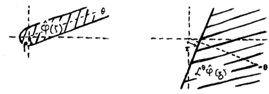
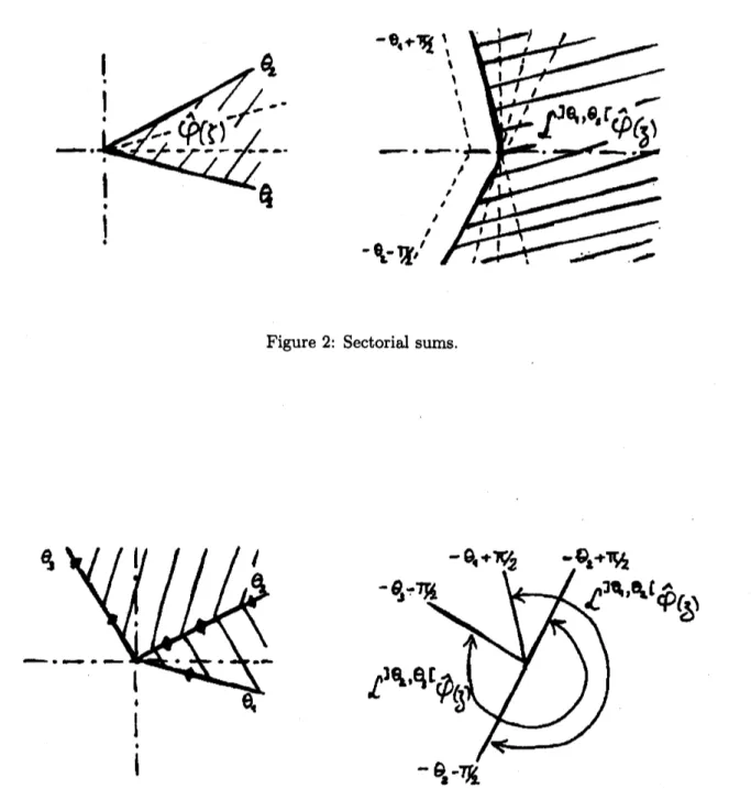
$Se\mathrm{c}$torial

sums

Suppose that $\hat{\varphi}(\zeta)$ converges

near

the origin and extends analytically to a sector

$\{\zeta\in \mathbb{C}|\theta_{1}<$

$\arg\zeta<\theta_{2}\}$ (where $\theta_{1},$$\theta_{2}\in \mathbb{R},$ $|\theta_{2}-\theta_{1}|<2\pi$), with exponential type less than $\tau$, then

we

can

movethedirection of integration$\theta \mathrm{i}\mathrm{n}\mathrm{s}\mathrm{i}\mathrm{d}\mathrm{e}$]$\theta_{1},$$\theta_{2}$[. According to the Cauchytheorem, $\mathcal{L}^{\theta’}\hat{\varphi}$ is the analytic continuation of$\mathcal{L}^{\theta}\hat{\varphi}$ when _{$|\theta’-\theta|<\pi$}, we can thus glue together these holomorphic

functionsandobtaina function$\mathcal{L}^{]\theta_{1},\theta_{2}[}\hat{\varphi}$

analyticintheunionof the half-planes $\{\Re e(z\mathrm{e}^{\mathrm{i}\theta})>\tau\}$,

which is

a

sectorial neighbourhood of infinity contained in $\{-\theta_{2}-\pi/2<\arg z<-\theta_{1}+\pi/2\}$

(see Figure 2). Notice however that, if$\theta_{2}-\theta_{1}>\pi$, the resulting function may be multivalued,

$i.e$

.

one

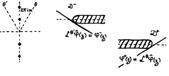
must consider the variable $z$ as moving on theRiemann surface of the logarithm.

A frequent situation is the following: $\hat{\varphi}=\mathcal{B}\tilde{\varphi}$ converges and extends analytically to several

infinite sectors, with bounded exponential type, but also has singularities at finite distance (in

particular $\hat{\varphi}$ hasfinite radius ofconvergence and

$\tilde{\varphi}$ is divergent). Then several “Borel-Laplace

sums” are available onvariousdomains, butare not the analyticcontinuations one of the other:

the presence of singularities, which separate the sectors one from the other, prevents onefrom

applying the Cauchy theorem. On theother hand, all these “sums” share the same asymptotic

expansion: the mutual differences are exponentially small in the intersection of their domains

of definition (see Figure 3).

(5)

Figure 2: Sectorial

sums.

Figure3: SeveralBorel-Laplacesums, analytic indifferent domains,may be attached toasingle

(6)

Resurgent

_functions

It is interesting to “measure” the singularities _{in the} $\zeta$-plane, since they

can

be considered

as

responsible for thedivergence ofthe

common

asymptotic expansion $\tilde{\varphi}(z)$ and for the

exponen-tially small differences between the various Borel-Laplace

sums.

The resurgent functions can

be defined

as

a class of formal series $\tilde{\varphi}$ such that the analytic continuation of the formal Borel

transform $\hat{\varphi}$ satisfies a certain

condition regarding the possible _{singularities, which makes it}

possible _{to develop a kind of singularity calculus} _(named _“alien _{calculus”).} _{These notions} _were

introduced in the late $70\mathrm{s}$ by J.

\’Ecalle,

who proved

their relevance in a number of analytic

problems [Eca81, _{Ma185]. We shall not} _{try to} _expound_{the theory in its full generality, but shall}

rather content ourselves withexplaininghow it works in thecase ofcertaindifference equations.

Note: The formal Borel transform of a series $\tilde{\varphi}(z)$ has positive radius ofconvergence if and

only if$\tilde{\varphi}(z)$ satisfies a “Gevrey-l” condition:

$\hat{\varphi}(\zeta)\in \mathbb{C}\{\zeta\}\Leftrightarrow\tilde{\varphi}(z)\in z^{-1}\mathbb{C}[[z^{-1}]]_{1}$ , where by

definition

$z^{-1}\mathbb{C}[[z^{-1}]]_{1}=$

{

_{$\sum_{n\geq 0}c_{n}z^{-n-1}|\exists\rho>0$}such that

$|c_{n}|=O(n!\rho^{n})$

}.

1.2 Linear and nonlinear

difference

equations

We shall be interested in formal series $\tilde{\varphi}$ solutions of certain equations involving the first-order

difference operator $\tilde{\varphi}(z)\mapsto\tilde{\varphi}(z+1)-\tilde{\varphi}(z)$ (orsecond-order differences). Thisoperator is well

defined in$\mathbb{C}[[z^{-1}]],$ _$e.g$. byway ofthe Taylor formula

$\tilde{\varphi}(z+1)-\tilde{\varphi}(z)=\partial\tilde{\varphi}(z)+\frac{1}{2!}\partial^{2}\tilde{\varphi}(z)+\frac{1}{3!}\partial^{3}\tilde{\varphi}(z)+\cdots$

,

(4)

where$\partial=\frac{\mathrm{d}}{\mathrm{d}z}$ andthe series is formally

convergent because of increasing valuations (wesay that

the series $\sum\frac{1}{r!}\partial^{f}\tilde{\varphi}$ is formally convergent because the right-hand side of

(4) is a well-defined

formal series, each coefficient of which is given by a finite sum of terms; this is the notion of

sequential convergence associated with the so-called Krulltopology).

It is elementary tocompute the counterpart of the differential and differenceoperatorsby$\mathcal{B}$:

$B$ : $\partial\tilde{\varphi}(z)-\rangle-\zeta\hat{\varphi}(\zeta)$, $\tilde{\varphi}(z+1)rightarrow \mathrm{e}^{-\zeta}\hat{\varphi}(\zeta)$

.

When$\tilde{\varphi}(z)$isobtainedbysolvinganequation, anaturalstrategy isthusto study

$\hat{\varphi}(\zeta)$

as

solution

of a transformed equation. If a Laplace transform $\mathcal{L}^{\theta}$

can

be applied to

$\hat{\varphi}$,

one

then

recovers

an

analytic solutionofthe original equation, because $\mathcal{L}^{\theta}\mathrm{o}B$ commuteswith the differential and

difference operators.

Two linear equations

Let

us

illustrate thison two simpleequations:

$\tilde{\varphi}(z+1)-\tilde{\varphi}(z)=a(z)$

,

$a(z)\in z^{-2}\mathbb{C}\{z^{-1}\}$ given, (5)

$\tilde{\psi}(z+1)-2\tilde{\psi}(z)+\tilde{\psi}(z-1)=b(z)$

,

$b(z)\in z^{-3}\mathbb{C}\{z^{-1}\}$ given. (6)

The correspondingequations for the formal Borel transforms are

(7)

$\theta_{\backslash }’\backslash$ $2|\iota\pi_{1\mathfrak{n}^{J}}|.\theta$ $\ovalbox{\tt\small REJECT}rightarrow$ 1 $ $’\gamma$ $\backslash \bullet$

,

$ $t$

,

$arrow—-\sim-\backslash |’arrow-\sim$ 1 1 $e$ $\uparrow$ $1$

1

Figure 4: Borel-Laplace summation for thedifferenceequation (5).

Here the power series \^a$(\zeta)$ and $\hat{b}(\zeta)$ converge to entire functions ofbounded exponential type

in every direction, vanishing at the origin;

moreover

$\hat{b}’(0)=0$

.

We thus get in $\mathbb{C}[[\zeta]]$ unique

solutions $\hat{\varphi}(\zeta)=\hat{a}(\zeta)/(\mathrm{e}^{-\zeta}-1)$ and $\hat{\psi}(\zeta)=\hat{b}(\zeta)/(4\sinh^{2\zeta})2$

’ which converge near the origin

and define meromorphic functions, the possible poles beinglocated in $2\pi \mathrm{i}\mathbb{Z}^{*}$

.

The original equations thus admit unique solutions$\tilde{\varphi}=\mathcal{B}^{-1}\hat{\varphi}$and $\tilde{\psi}=B^{-1}\hat{\psi}$in $z^{-1}\mathbb{C}[[z^{-1}]]$

.

For each ofthem, Borel-Laplace summation is possibleand weget two natural sums, associated

with two sectors:

$\varphi^{+}(z)=\mathcal{L}^{\theta}\hat{\varphi}(z)$, $\theta\in]-\frac{\pi}{2},$$\frac{\pi}{2}[, \varphi^{-}(z)=\mathcal{L}^{\theta’}\hat{\varphi}(z), \theta’\in]\frac{\pi}{2},3\tau\pi[$ ,

and similarly $\hat{\psi}(\zeta)$ gives rise to _{$\psi^{+}(z)$} and _{$\psi^{-}(z)$}

.

The functions $\varphi^{+}$ and $\psi+\mathrm{a}\mathrm{r}\mathrm{e}$ solutions of (5) and (6), analytic in a domain of the form

$D^{+}=\mathbb{C}\backslash \{\mathrm{d}\mathrm{i}\mathrm{s}\mathrm{t}(z,\mathbb{R}^{-})\leq ar\}$

.

Thesolutions $\varphi^{-}$ and $\psi^{-}$ aredefined in

a

symmetric domain$D^{-}$

(see Figure 4). The intersection $D^{+}\cap D^{-}$ hae two connected components, _{$\{\Im mz<-\mathcal{T}\}$} and

$\{\Im mz>\tau\}$. In thecaseofequation (5) for instance, theexponentiallysmalldifference$\varphi^{+}-\varphi^{-}$

in the lower component is related to thesingularities of$\hat{\varphi}$ in$2\pi \mathrm{i}\mathrm{N}^{*};$ it

can

beexactlycomputed

by the resiuduum formula: the singularity at $\omega=2\pi \mathrm{i}m$yieldsacontribution

A $\mathrm{e}^{-}"$, with _{$A_{\omega}=-2\pi \mathrm{i}\hat{a}(\omega)$}

(the modulus of which is $|A_{\omega}|\mathrm{e}^{2\pi m\Im mz}$, which is exponentially small for $\Im mzarrow-\infty$); _the

difference $( \varphi^{+}-\varphi^{-})(z)=\int_{\mathrm{e}^{\mathrm{i}\theta}\infty}^{\mathrm{e}^{\mathrm{i}\theta}\infty},\hat{\varphi}(\zeta)\mathrm{e}^{-z\zeta}\mathrm{d}\zeta$ is simply the

sum

ofthese contributions:

$\varphi^{+}(z)-\varphi^{-}(z)=‘\sum_{v\in 2\pi \mathrm{i}\mathrm{N}^{*}}A_{\omega}\mathrm{e}^{-\omega z}$, $\Im mz<-\tau$ (7)

as

is easily seen by deforming the contour of integration (choose $\theta$ and $\theta’$ close enough to _$\pi/2$

accordingto theprecise location of$z$, and pushthe contour of integration upwards).

Symmetri-cally, thedifferenceinthe upper component canbecomputedfrom the singularities $\mathrm{i}\mathrm{n}-2\pi \mathrm{i}\mathrm{N}^{*}$

.

Note: $\varphi^{+}(z)$ is theuniquesolution of(5)which tends to$0$when$\Re ezarrow+\infty$and

can

be written

(8)

$\Re ezarrow-\infty$; the difference defines _two _1-periodic _{functions, the} _Fourier

coefficients of which

can be expressed _{in term of the Fourier transform of} $a(\pm \mathrm{i}\rho+z)$ (take _$\rho>0$ large enough).

One

recovers

theprevious_{formula for the difference by using}_{the integral representation} _for_the

Borel transform to compute the numbers \^a$(\omega)$

.

Nonlinear equations

In the present text we shall showhowone can deal with nonlinear difference equations like

$\tilde{\varphi}(z+1)-\tilde{\varphi}(z)=a(z+\tilde{\varphi}(z))$, $a(z)\in z^{-2}\mathbb{C}\{z^{-1}\}$ given, (8)

which is related to Abel’s equation and theclassification of holomorphic germs inone complex

variable, or

$\tilde{\psi}(z+1)-2\tilde{\psi}(z)+\tilde{\psi}(z-1)=b(\tilde{\psi}(z),\tilde{\psi}(z-1))$, (9)

with certain $b(x, y)\in \mathbb{C}\{x, y\}$, which is related to splitting problems in two complex variables.

Dealing with nonlinear equations will require thestudyof convolution,which is the subject

of sections 1.3 and 1.4. The Borel transforms $\hat{\varphi}(\zeta)$ and $\hat{\psi}(\zeta)$ will still be holomorphic at the

origin but

no

longer meromorphic in $\mathbb{C}$, as will be shown later; their analytic continuations

have

more

complicated singularities than mere first- or second-order poles. We shall introduce

alien calculus in Section 2 and a more general version of it in Section 3.3 to deal with these

singularities.

1.3 The

Riemann

surface

$R$

and the

analytic

continuation of convolution

The first nonlinear operation tobe studied is the multiplication offormal series.

Lemma 1 Let$\hat{\varphi}$ and

th

denote the

_formal

Borel

_transforms

_of

$\tilde{\varphi},\tilde{\psi}\in z^{-1}\mathbb{C}[[z^{-1}]]$ and consider

the prvduct series$\tilde{\chi}=\tilde{\varphi}\tilde{\psi}$

.

Then its

forrnal

Bord

_transform

is given by the “convolution”

$(B \tilde{\chi})(\zeta)=(\hat{\varphi}*\hat{\psi})(\zeta)=\int_{0}^{\zeta}\hat{\varphi}(\zeta_{1})\hat{\psi}(\zeta-\zeta_{1})\mathrm{d}\zeta_{1}$

.

(10)

The above formula must be interpreted termwise: $\int_{0n!}^{\zeta\zeta^{n}}\perp\frac{(\zeta-\zeta_{1})^{\mathrm{n}}}{m!},\mathrm{d}\zeta_{1}=\frac{\zeta^{n+m+1}}{(n+m+1)!}$ (as can be

checked $e.g$

.

by inductionon $n$, which is sufficient toprove the lemma).

The$p$rvblem

of

analytic continuation

The formula

can

be given

an

analytic meaning in the

case

of Gevrey-l formal series: if$\hat{\varphi},\hat{\psi}\in$

$\mathbb{C}\{\zeta\}$, their convolution is convergent inthe intersection of the discs ofconvergence of$\hat{\varphi}$ and

di

and defines a new holomorphic germ $\hat{\varphi}*\hat{\psi}$ at the origin; formula (10) then holds as a relation

between holomorphic functions, but only for $|\zeta|$ small enough (smaller than theradii of

conver-gence of $\hat{\varphi}$ and $\hat{\psi}$). What about the analytic continuation of$\hat{\varphi}*\hat{\psi}$ when $\hat{\varphi}$ and $\hat{\psi}$ themselves

admitananalytic continuation beyondtheir discs ofconvergence? What about the

case

when$\hat{\varphi}$

and

_th

extend to meromorphic functions for instance?

A preliminary

answer

is that $\hat{\varphi}*\hat{\psi}$ always admit ananalytic continuation in the intersection

of the “holomorphicstars” of $\hat{\varphi}$ and

$\hat{\psi}$

.

We define the

holomorphic star ofagerm

as

the union

(9)

are star-shaped withrespect to the origin $(i.e. \forall\zeta\in U, [0, \zeta]\subset U)$

.

And it is indeed clear that

if $\hat{\varphi}$ and

$\hat{\psi}$

are

holomorphic in such a _$U$, formula (10) makes

sense

for

all $\zeta\in U$ and provides

the analytic continuation of$\hat{\varphi}*\hat{\psi}$

.

With aview to further use we notice that, if

$|\hat{\varphi}(\zeta)|\leq\Phi(|\zeta|)$

and $|\hat{\psi}(\zeta)|\leq\Psi(|\zeta|)$ for all _{$\zeta\in U$}, then

$|\hat{\varphi}*\hat{\psi}(\zeta)|\leq\Phi*\Psi(|\zeta|)$, _{$\zeta\in U.$} (11)

The next step is to study what happens on singular rays, behind singular points. The idea

is that convolution ofpoles generates ramification $(” \mathrm{m}\mathrm{u}\mathrm{l}\mathrm{t}\mathrm{i}\mathrm{v}\mathrm{a}\mathrm{l}\mathrm{u}\mathrm{e}\mathrm{d}\mathrm{n}\mathrm{e}\mathrm{s}\mathrm{s}" )$ but is easy to continue

analytically. For example, since

$1* \hat{\varphi}(\zeta)=\int_{0}^{\zeta}\hat{\varphi}(\zeta_{1})\mathrm{d}\zeta_{1}$,

we

see

that when $\hat{\varphi}$ is a meromorphic function with poles in

a

set $\Omega\subset \mathbb{C}^{*},$ $1*\hat{\varphi}$ admits

an

analytic continuation along any path issuingfrom the origin and avoidingSt; in other words, it

defines a functionholomorphic

on

the universal

cover3

of$\mathbb{C}\backslash \Omega$

,

with logarithmic singularities

at the poles of$\hat{\varphi}$

.

But convolution may also create

new

singular points. For instance, if $\hat{\varphi}(\zeta)=\frac{1}{(-\omega}$, and

$\hat{\psi}(\zeta)=\frac{1}{\zeta-\omega},$, with$\omega’,\omega’’\in \mathbb{C}^{*}$, one gets

$\hat{\varphi}*\hat{\psi}(\zeta)=\frac{1}{\zeta-\omega}(\int_{0}^{\zeta}\frac{\mathrm{d}\zeta_{1}}{\zeta_{1}-\omega’}+\int_{0}^{\zeta}\frac{\mathrm{d}\zeta_{1}}{\zeta_{1}-\omega’’})$ , $\omega=\omega’+\omega’’$

.

We thushavelogarithmic singularities at$\omega’$ and$\omega’’$, but alsoa

pole at $\omega$, the residuum of which

is an integer multiple of$2\pi \mathrm{i}$ which depends

on

the path chosen to approach

$\omega$

.

In other words, $\hat{\varphi}*\hat{\psi}$extends meromorphically to the universal

cover

of

$\mathbb{C}\backslash \{\omega’,\omega’’\}$, with a pole lying

over

$\omega$

(the residuum ofwhich depends on the

sheet4

ofthe Riemann surface which is considered; in

particular it vanishes for the principal

sheet5

if$\arg\omega’\neq\arg\omega’’$, which is consistent with what

was previouslysaid on the holomorphic star).

The Riemann

_surface

$\mathcal{R}$

With

a

view to the difference equations we

are

interested in and to the expected behaviour of

the Borel transforms, we definea Riemann surface which is obtained by adding a point to the

universal

cover

of$\mathbb{C}\backslash 2\pi \mathrm{i}$Z.

3 _Here_it_{is understood} _{that the base.point}_{is at} _{the origin. If}$\Omega$isa closed subset of$\mathbb{C}$with$\mathbb{C}\backslash \Omega$connected

and $\zeta 0\in \mathbb{C}\backslash \Omega$, the universalcover of$\mathbb{C}\backslash \Omega$with base-point $\zeta 0$ can be definedas the set of homotopyclasses of

$\mathrm{p}\mathrm{a}\underline{\mathrm{t}\mathrm{h}\mathrm{s}}$issuingfrom$\zeta 0$ andlying in

$\mathbb{C}\backslash \Omega$(

$\mathrm{e}\underline{\mathrm{q}\mathrm{u}\mathrm{i}\mathrm{v}}\mathrm{a}\mathrm{l}\mathrm{e}\mathrm{n}\mathrm{c}\mathrm{e}$classes forhomotopywith fixedextremities). We denote it

$(\mathbb{C}\backslash \Omega, \zeta 0)$

.

There isacovering map$\pi$: $(\mathbb{C}\backslash \Omega, \zeta 0)arrow \mathbb{C}\backslash \Omega$,which associates with any class$c$the extremity$\gamma(1)$

of$\mathrm{a}\mathrm{n}\underline{\mathrm{y}\mathrm{p}\mathrm{a}\mathrm{t}}\mathrm{h}\gamma$ :

$[0,1]arrow \mathbb{C}\backslash \Omega$which represents $c$, and which allows one todefine a Riemannsurface structure

on$(\mathbb{C}\backslash \Omega, \zeta 0)$by pullingbackthe complex structure of$\mathbb{C}\backslash \Omega$(see [CNP93,pp. 81-89and 105-112]). Forexample,

the Riemann surfaceofthe logarithm is $(\mathbb{C}\backslash \{0\}, 1)$, thepointsof which canbewritten “$r\mathrm{e}^{\mathrm{i}\theta}$”

with $f>0$ and

$\mathit{9}\in$R. We oftenusetheletter$\zeta$for pointsofauniversal cover, and then denote by $\zeta=\pi(\zeta)$ their projection.

4Againwecantake the base-point at the origin to define theuniversalcoverof$\mathbb{C}\backslash \Omega$, here with$\Omega=\{\omega‘, \omega’’\}$

.

The word “sheets” usuallyrefers to the various lifts in thecoverofanopensubset $U$of thebasespace which is

star-shapedwithrespectto oneof its $\underline{\mathrm{p}\mathrm{o}\mathrm{i}\mathrm{n}\mathrm{t}\mathrm{s}},$$i.e$

.

tothevarious connectedcomponentsof$\pi^{-1}(U)$

.

5In thecaseofa universalcover $(\mathbb{C}\backslash \Omega, \zeta 0)$, the “principal sheet” $\tilde{U}$

isobtainedbyconsidering the maximal open subset$U$of$\mathbb{C}\backslash \Omega$ which isstar-shaped withrespectto$\zeta 0$ andliftingitbymeansof rectilinearsegments: $\tilde{U}$

(10)

Definition 3 Let$\mathcal{R}$ be theset

of

all homotopy classes

_of

paths issuing

_from

the $\mathit{0}$rigin and lyin9

znside $\mathbb{C}\backslash 2\pi \mathrm{i}\mathbb{Z}$ (except

for

their initialpoint), and let

$\pi$ : $\mathcal{R}arrow \mathbb{C}\backslash 2\pi \mathrm{i}\mathbb{Z}^{*}$ be the covering map,

whichassociates with any class$c$ the extremity$\gamma(1)$

of

anypath$\gamma$ : $[0,1]$ —

$\mathbb{C}$ which represents

$c$

.

We consider$\mathcal{R}$ as a Riemann

surface

by pulling back by$\pi$ the complex structure

of

$\mathbb{C}\backslash 2\pi \mathrm{i}\mathbb{Z}^{*}$.

Observe that $\pi^{-1}(0)$ consists of only one point (the homotopy class of the constant _path),

which we may call the origin of$\mathcal{R}$

.

Let _$U$ be the complex plane

deprived from the half-lines

$+2\pi \mathrm{i}[1,$$+\infty$[ and $-2\pi \mathrm{i}[1,$$+\infty$[. We define the “principal sheet” of $\mathcal{R}$ as the set of all the

classes ofsegments $[0, \zeta],$ $\zeta\in U$; equivalently, it is the connected component of$\pi^{-1}(U)$ which

contains the origin. We define the “half-sheets” of $\mathcal{R}$ as the various connected components

of$\pi^{-1}(\{\Re e\zeta>0\})$ or of$\pi^{-1}(\{\Re e\zeta<0\})$

.

A holomorphic function of$\mathcal{R}$ can beviewed as a germof holomorphic

functionat theorigin

of$\mathbb{C}$ which admits analytic continuation

along any path avoiding $2\pi \mathrm{i}\mathbb{Z}$; we then say that this

germ “extends holomorphically to $\mathcal{R}$”. This definition a

priori does not authorize analytic

continuation along

a

path which leads to the origin, unless this path stays in the principal

sheet6.

More precisely, one canprove

Lemma 2

_If

$\Phi$ is holomorphic in$\mathcal{R}$, then its restriction to the

principal sheet

_defines

a

holo-mo$r\mathrm{p}hic$

function

$\varphi$

of

$U$ which extends analytically along any path

$\gamma$ issuing

ffom

$0$ and lying

in$\mathbb{C}\backslash 2\pi \mathrm{i}$Z. The analytic continuation is given by

$\varphi(\gamma(t))=\Phi(\Gamma(t))$, where $\Gamma$ is the

lift of

$\gamma$

which starts at the $or\dot{\tau}gin$

of

R.

Conversely, given $\varphi\in \mathbb{C}\{\zeta\}$,

if

any $c\in \mathcal{R}$ can be represented by a path

of

andytic

contin-uation

_for

$\varphi$, then the value

of

$\varphi$ at the extremity 7(1)

of

this path depends only

on

$c$ and the

formula

$\Phi(c)=\varphi(\gamma(1))$

defines

a holomorphic

function of

72.

The absence of singularity at the originonthe principalsheetistheonlydifference between$R$

and the universal

cover

of$\mathbb{C}\backslash 2\pi \mathrm{i}\mathbb{Z}$ withbase-point at 1. For instance, among thetwo series

$\sum_{m\in \mathrm{z}*}\frac{1}{\zeta}\mathrm{e}^{-|m|\int_{1}^{\zeta}\frac{\mathrm{d}\zeta_{1}}{\zeta_{1}-2\pi \mathrm{i}m}}$, $\sum_{m\in \mathrm{z}*}\frac{1}{\zeta}\mathrm{e}^{-|m|\int_{0}^{\zeta}\frac{\mathrm{d}\zeta_{1}}{\zeta_{1}-2\pi \mathrm{i}m}}$,

the first

one

defines a functionwhich is holomorphic in the universal cover of$\mathbb{C}\backslash 2\pi \mathrm{i}\mathbb{Z}$ but not

in$\mathcal{R}$, whereas the second

one defines a holomorphic function of R.

Analytic continuation

_of

convolution in 72

The main result of this section is

Theorem 1

_If

twogems at the $\mathit{0}$rigin eztend holomorphically to$\mathcal{R}$, so does their convolution

product.

Idea

_of

the proof. Let $\hat{\varphi}$ and $\hat{\psi}$ be

holomorphic germs at the origin of$\mathbb{C}$ which admit analytic

continuation along anypath avoiding $2\pi \mathrm{i}\mathbb{Z}$; we denote by the same symbolsthe corresponding

$\overline{\epsilon_{\mathrm{T}\mathrm{h}\mathrm{a}\mathrm{t}\mathrm{i}\S},}$_unlaes_it _{lies in}

$U=\mathbb{C}\backslash \pm 2\pi \mathrm{i}\lfloor 1,$$+\infty$[. We shall often identify the paths issuing$\mathrm{h}\mathrm{o}\mathrm{m}0$in$\mathbb{C}\backslash 2\pi \mathrm{i}\mathrm{Z}$

andtheirliftsstarting atthe origin of R. Sometimes,weshallevenidentifyapoint of$\mathcal{R}$with its projection by$\pi$

(thepath which leads tothispoint being understood), which amounts totreating aholomorphic function of$\prime \mathcal{R}$ as amultivalued functionon$\mathbb{C}\backslash 2\pi \mathrm{i}$Z.

(11)

holomorphic functions of$\mathcal{R}$

.

One could be tempted to think that, if a point

$\zeta$ of $\mathcal{R}$ is defined

by

a

path $\gamma$, the integral

$\hat{\chi}(\zeta)=\int_{\gamma}\hat{\varphi}(\zeta’)\hat{\psi}(\zeta-\zeta’)\mathrm{d}\zeta’$ (12)

would give the value of the analytic continuation of $\hat{\varphi}*\hat{\psi}$ at

$\zeta$

.

However, this formula does

not always make sense, since one must worry about the path $\gamma’$ followed by _{$\zeta-\zeta’$} when $\zeta’$

follows $\gamma$: is

$\hat{\psi}$ definedonthispath? Infact, even

if

_7‘

liesin$\mathbb{C}\backslash 2\pi \mathrm{i}\mathbb{Z}$ (and thus$\hat{\psi}(\zeta-\zeta’)$ makes

sense), even if$\gamma’$ coincides with

$\gamma$

,

it may happen that this integral does not give the analytic

continuation of$\hat{\varphi}*\hat{\psi}$ at

$\zeta$ (usually, the value of thisintegral does not dependonly on

$\zeta$ but also

on

the path$\gamma)^{7}$

.

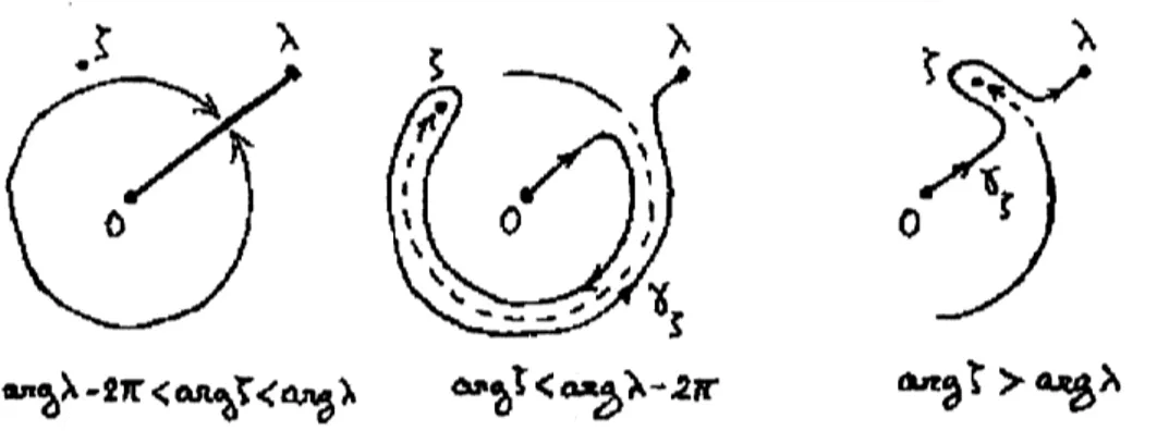
The construction of the desired analytic continuation relies on the idea of “symmetrically

contractile” paths. A path $\gamma$ issuing from $0$ is said to be

$\mathcal{R}$-symmetric if it lies in

$\mathbb{C}\backslash 2\pi \mathrm{i}\mathbb{Z}$

(except for its starting point) and is symmetric with respect to its midpoint: the paths $t\in$ $[0,1]rightarrow\gamma(1)-\gamma(t)$ and $t\in[0,1]rightarrow\gamma(1-t)$ coincide up to reparametrisation. A path is said

to be $\mathcal{R}$-symmetrically contractile if it is $\mathcal{R}$-symmetric and

can

be continuously deformed and

shrunk to $\{0\}$ within the class of$\mathcal{R}$-symmetric paths. The main point is that any

point of$\mathcal{R}$

can be defined by an $\mathcal{R}$-symmetrically contractile path. More

precisely:

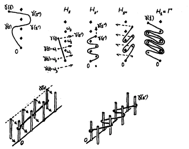
Lemma 3 Let$\gamma$ be a path issuing

from

$0$ and lying in $\mathbb{C}\backslash 2\pi \mathrm{i}\mathbb{Z}$ (except

for

its startingpoint).

Then there exists an $\mathcal{R}$-symmetrically contractile path $\Gamma$ which is homotopic to

$\gamma$

.

Moreover,

one can construct$\Gamma$ so that there is a continuous map

$(s,t)\mapsto H(s,t)=H_{s}(t)$ satisfying

$i)H_{0}(t)\equiv 0$ and$H_{1}(t)\equiv\Gamma(t)$,

$ii)$ each $H_{s}$ is an $\mathcal{R}$-symmetricpath utith$H_{s}(0)=0$ and

$H_{s}(1)=\gamma(s)$

.

We shall not try to write

a

formal proof of this lemma, but it is easy to visualize

a

way

of constructing $H$

.

Let a point $\zeta=\gamma(s)$ move along $\gamma$ (as $s$ varies from $0$ to 1) and remain

connected to $0$ by an extensible thread, with moving nails pointing downwards at each point

of $\zeta-2\pi \mathrm{i}\mathbb{Z}$, while fixed nails point upwards at each point of $2\pi \mathrm{i}\mathbb{Z}$ (imagine for

instance

that

the first nails arefastened to amoving rule and the last ones to a fixed rule). As $s$ varies, the

thread is progressively stretched but it has to meander between the nails. The path $\Gamma$ is given

by the thread inits finalform, when$\zeta$ has reached the extremity of7;the paths _{$H_{s}$} correspond

to the thread at intermediary

stages8

(see Figure 5).

It is now easy to end theproofofTheorem 1. Given $\hat{\varphi},\hat{\psi}\wedge$ as above and

$\gamma$ apath of$\mathcal{R}$ along

which we wish to follow the analytic continuation of$\hat{\varphi}*\psi$, we take $H$ as in Lemma3 and let

the reader convince himselfthat the formula

$\hat{\chi}(\zeta)=\int_{H_{\delta}}\hat{\varphi}(\zeta’)\hat{\psi}(\zeta-\zeta’)\mathrm{d}\zeta’$, $\zeta=\gamma(s)$, (13)

defines the analytic continuation $\hat{\chi}$ of$\hat{\varphi}*\hat{\psi}$along

$\gamma$ (in thisformula, $\zeta’$ and$\zeta-\zeta’$ move onthe

same

path $H_{s}$ which avoids $2\pi \mathrm{i}\mathbb{Z}$

,

by $\mathcal{R}$-symmetry). See

[Eca81, Vol. 1], [CNP93], [GSOI] for

more

details. $\square$

7_However,_if

_zb

_is_entire,_{it is}_true_that_the_{integral (12)} _does_provide_{the analytic continuation of}$\hat{\varphi}*\hat{\psi}$along

7.

8Notethat the mere existence of acontinuous $H$ satisfying conditions :) and $ii$) implies that $\gamma$ and $\Gamma$ are

homotopic, asis visually clear (theformula

$h_{\lambda}(t)=H(\lambda+(1-\lambda)t,$ $\frac{t}{\lambda+(1-\lambda)t})$, $0\leq\lambda\leq 1$

(12)

$H_{\mathrm{g}\bullet}$

Figure 5: Construction ofan $\mathcal{R}$-symmetrically contractile path $\Gamma$ homotopic to

(13)

Ofcourse, if the path $\gamma$ mentionedin the last part ofthe proofstays in the principal sheet

of $\mathcal{R}$, the analytic continuation is simply given by formula

(10). Inparticular, if$\hat{\varphi}$ and

di

have

bounded exponential type in a direction $\arg\zeta=\theta,$ $\theta\not\in\frac{\pi}{2}+\pi \mathbb{Z}$, it follows from inequality (11)

that $\hat{\varphi}*\hat{\psi}$ has the same property.

1.4

Formal

and convolutive models

of

the

algebra of resurgent

functions,

$\tilde{\mathcal{H}}$

and

$\hat{\mathcal{H}}(\mathcal{R})$

In view of Theorem 1, the convolution of germs induces

an

internal law on the space of

holo-morphic functions of$R$, which is commutative and associative (beingthe counterpart of

multi-plication offormal series, by Lemma 1). In fact, we havea commutative algebra (withoutunit),

which can be viewed

as

a subalgebra of the convolution algebra $\mathbb{C}\{\zeta\}$, and which corresponds

via $B$ to asubalgebra (for the ordinary product offormalseries) of_{$z^{-1}\mathbb{C}[[z^{-1}]]$}

.

Deflnition 4 The space $\hat{\mathcal{H}}(\mathcal{R})$

of

allholomorphic

_{functions of}

$\mathcal{R}$, equippedunth

the convolution

product, is an algebra called the convolutive model

_of

the algebra

_of

resurgent

_functions.

The subalgebra $\tilde{\mathcal{H}}=\mathcal{B}^{-1}(\hat{\mathcal{H}}(R))$

of

$z^{-1}\mathbb{C}[[z^{-1}]]$ is called the multiplicative model

of

the algebra

of

resungent

_functions.

Theformal series in$\tilde{\mathcal{H}}$

(most of which have zeroradius ofconvergence) arecalled “resurgent

functions”. These definitions will in fact be extended to

more

general objects in the following

(see Section 3 on “singularities”).

Thereis no unit for the convolution in$\hat{\mathcal{H}}(\mathcal{R})$

.

Introducing a newsymbol _$\delta=B1$, we

extend

the formal Borel transform:

$B$ :

$\tilde{\chi}(z)=c_{0}+\sum_{n\geq 0}c_{n}z^{-n-1}\in \mathbb{C}[[z^{-1}]]rightarrow\hat{\chi}(\zeta)=c_{0}\delta+\sum_{n\geq 0}\mathrm{c}_{n}\frac{\zeta^{n}}{n!}\in \mathbb{C}\delta\oplus \mathbb{C}[[\zeta]]$,

and also extend convolution from $\mathbb{C}[[\zeta]]$ to C6$\oplus \mathbb{C}[[\zeta]]$ linearly, by treating

5

as a unit ($i.e$

.

so

as

tokeep $B$ amorphism ofalgebras). This way, $\mathbb{C}\delta\oplus\hat{\mathcal{H}}(\mathcal{R})$ is an algebrafor the convolution,

which is isomorphic via$B$ to the algebra $\mathbb{C}\oplus\tilde{\mathcal{H}}$

.

Observe that

$\mathbb{C}\{z^{-1}\}\subset \mathbb{C}\oplus\tilde{\mathcal{H}}\subset \mathbb{C}[[z^{-1}]]_{1}$

.

Having dealt with multiplication of formalseries, we

can

study compositionand its image in

$\mathbb{C}\delta\oplus\hat{\mathcal{H}}(\mathcal{R})$:

Proposition 1 Let $\tilde{\chi}\in \mathbb{C}\oplus\tilde{\mathcal{H}}$. Then composition by

$zrightarrow z+\tilde{\chi}(z)$

defines

a linear

opera-tor

_of

$\mathbb{C}\oplus\tilde{\mathcal{H}}$ into itself, and

for

any $\tilde{\psi}\in\tilde{\mathcal{H}}$ the Borel

transform of

$\tilde{\alpha}(z)=\tilde{\psi}(z+\tilde{\chi}(z))=$

$\sum_{\gamma\geq 0}\frac{1}{r!}\partial^{f}\tilde{\psi}(z)\tilde{\chi}^{r}(z)$ is given by the series

of

functions

a

$( \zeta)=\sum_{r\geq 0}\frac{1}{r!}((-\zeta)^{r}\hat{\psi}(\zeta))*\hat{\chi}^{*r}(\zeta)$ (14)

(where $\hat{\chi}=B\tilde{\chi}$ and$\hat{\psi}=\mathcal{B}\tilde{\psi}$), whichis uniformly convergent in every compact subset

(14)

The _{convergence of the series stems from the regularizing character of convolution} (the

convergence in the principal sheet of lre can be proved by

use

of (11); see [Eca81, Vol. 1]

or [CNP93] for the convergence in thewhole Riemann surface).

The notation $\hat{\alpha}=\hat{\psi}\mathrm{O}*(\delta’+\hat{\chi})$ andthename “composition-convolution” are

usedin [Ma195], with a symbol $\delta’=Bz$ which must be considered as _{the derivative of}$\delta$

.

The symbols $\delta$ and $\delta$‘

will be interpreted as elementary singularities in Section 3.

In Proposition 1, the operator of composition by $zrightarrow z+\tilde{\chi}(z)$ is invertible; in fact, $\mathrm{I}\mathrm{d}+\tilde{\chi}$

has a well-defined inverse forcomposition in $\mathrm{I}\mathrm{d}+\mathbb{C}[[z^{-1}]]$, which turnsout to be also resurgent:

Proposition 2

_If

$\tilde{\chi}\in \mathbb{C}\oplus\tilde{\mathcal{H}}$, the

formal transformation

$\mathrm{I}\mathrm{d}+\tilde{\chi}$ has an inverse (for composition)

of

the

_form

$\mathrm{I}\mathrm{d}+\tilde{\varphi}$ with $\tilde{\varphi}\in\tilde{\mathcal{H}}$

.

This can be proven by the

same

arguments as Proposition 1, since the Lagrange inversion

formula allows

one

to write

$\tilde{\varphi}=\sum_{k\geq 1}\frac{(-1)^{k}}{k!}\partial^{k-1}(\tilde{\chi}^{k})$, hence $\hat{\varphi}=-\sum_{k\geq 1}\frac{\zeta^{k-1}}{k!}\hat{\chi}^{*k}$

.

(15)

One canthus think of$zrightarrow z+\tilde{\chi}(z)$

as

ofa “resurgent change of variable”.

Similarly, substitution of

a

resurgent functionwithout constant term into

a

convergent series

is possible:

Proposition 3

_If

$C(w)= \sum_{n\geq 0}C_{n}w^{n}\in \mathbb{C}\{w\}$ and$\tilde{\psi}\in\tilde{\mathcal{H}}$, then the

formd

$se\sqrt esC\mathrm{o}\tilde{\psi}(z)=$ $\sum_{n\geq 0}C_{n}\tilde{\psi}^{n}(z)$ belongs to $\mathbb{C}\oplus\tilde{\mathcal{H}}$

.

The proofconsists in verifying the convergence of the series $B(C \mathrm{o}\tilde{\psi})=\sum_{n\geq 0}C_{n}\hat{\psi}^{\mathrm{x}n}$

.

As a consequence, any resurgent function with

nonzero

constant term has a resurgent

mul-tiplicative inverse: $1/(c+ \tilde{\psi})=\sum_{n\geq 0}(-1)^{n}c^{-n-1}\tilde{\psi}^{n}\in \mathbb{C}\oplus\tilde{\mathcal{H}}$

.

The exponential ofa resurgent

function$\tilde{\psi}$is also a

resurgent function, the Borel transformof which is the convolutive

exponen-tial

$\exp_{*}(\hat{\psi})=\delta+\hat{\psi}+\frac{1}{2!}\hat{\psi}*\hat{\psi}+\frac{1}{3!}\hat{\psi}*\hat{\psi}*\hat{\psi}+\ldots$

(in this

case

the substitution is well-defined even if $\tilde{\psi}(z)$ has a constant term).

We end this section by remarking that the role of the lattice $2\pi \mathrm{i}\mathbb{Z}$ in the definition of_$R$ is

not essential in the theory of resurgentfunctions. See Section 3.3for amoregeneraldefinition of

the spaceofresurgentfunctions (inwhich the location ofsingularpointsis not apriorirestricted

to$2\pi \mathrm{i}\mathbb{Z}$), witha property ofstabilityby convolutionasinTheorem 1, and with alien derivations

more general than the ones to be defined in Section 2.3.

2 Alien

calculus and Abel’s

equation

We

now

turn to the resurgent treatment of the nonlinear first-order difference equation (8),

(15)

2.1 Abel’s equation and tangent-to-identity holomorphic

germs

of

$(\mathbb{C}, 0)$

One of the origins of

\’Ecalle’s

work on Resurgence _{theory is the problem of the classification}

of holomorphic germs $F$ of $(\mathbb{C}, 0)$ in the “resonant” case. This is the question, important

for one-dimensional complex dynamics, of describing the conjugacy classes of the group $\mathrm{G}$ of

local analytic transformations $w\mapsto F(w)$ which are $1\mathrm{o}c$ally invertible, _$i.e$. of the form

$F(w)=$

$\lambda w+O(w^{2})\in \mathbb{C}\{w\}$with$\lambda\in \mathbb{C}^{*}$. It iswell-knownthat, ifthemultiplier

$\lambda=F’(0)$ has modulus

$\neq 1$, then$F$ is holomorphically linearizable: there exists$H\in \mathrm{G}$ such that_{$H^{-1}\mathrm{o}F\mathrm{o}H(w)=\lambda w$}

.

Resurgence comes into play when we consider the resonant case, $i.e$. when $F’(\mathrm{O})$ is a root of

unity (the so-called “small divisor problems”, which appear when $F’(\mathrm{O})$ has modulus 1 but is

not aroot of unity,

are

ofdifferent nature–see S. Marmi’s lecture in this volume).

Thereferences forthis part of the text

are:

[Eca81, Vol. 2], [Eca84], [Ma185] (and Example1

of [Eca05] p. 235). For non-resurgent approaches of the

same

problem,

see

[MR83], [DH84],

[Shi98], [ShiOO], [Mi199], [Lor06].

Non-degenerate parabolic germs

Here, for simplicity, we limit ourselves to $F’(\mathrm{O})=1,\acute{\iota}.e$

.

to germs $F$ which are tangent to

identity, with the further requirement that $F”(0)\neq 0$, a condition which is _easily seen _{to be}

invariant by conjugacy. Rescaling the variable $w$ if necessary,

one

can suppose $F”(0)=2$

.

It

will be

more

convenient to work “near infinity”, $i.e$

.

to

use

the variable z—-l/w.

Definition 5 We call “non-degenerate parabolic germ at the $\mathit{0}\dot{n}gin’$’

any

$F(w)\in \mathbb{C}\{w\}$

of

the

form

$F(w)=w+w^{2}+O(w^{3})$

.

We call “non-degenerate parabolic gern at infinity” a

_{transformation}

$zrightarrow f(z)$ which is

conju-gated by $z=-1/w$ to a non-degenerateparabolic germ $F$ at the origin:

$f(z)=-1/(F(-1/z))$,

$i.e$

.

any$f(z)=z+1+a(z)$ urith $a(z)\in z^{-1}\mathbb{C}\{z^{-1}\}$

.

Let $\mathrm{G}_{1}$ denote the subgroup of

$\mathrm{t}\mathrm{a}\mathrm{n}\mathrm{g}\mathrm{e}\mathrm{n}\mathrm{t}- \mathrm{t}\infty \mathrm{i}\mathrm{d}\mathrm{e}\mathrm{n}\mathrm{t}\mathrm{i}\mathrm{t}\mathrm{y}$germs. One can easily check that, if

$F,$$G\in \mathrm{G}_{1}$ and $H\in \mathrm{G}$, then $G=H^{-1}\circ F\circ H$ implies _{$G”(\mathrm{O})=H’(\mathrm{O})F’’(\mathrm{O})$}. In order to work

with non-degenerate parabolic germs only, we can thus restrictourselves to$\mathrm{t}\mathrm{a}\mathrm{n}\mathrm{g}\mathrm{e}\mathrm{n}\mathrm{t}- \mathrm{t}\mathrm{t}\succ \mathrm{i}\mathrm{d}\mathrm{e}\mathrm{n}\mathrm{t}\mathrm{i}\mathrm{t}\mathrm{y}$

conjugating transformations $H,$ $i.e$

.

we

can

content ourselves with studying the adjoint action

of$\mathrm{G}_{1}$

.

It turns out that formal transformations also play a role. Let $\tilde{\mathrm{G}}_{1}$

denote the group (for

composition) offormal series ofthe form $\tilde{H}(w)=w+O(w^{2})\in \mathbb{C}[[w]]$

.

It may happenthat two

parabolic germs $F$and$G$ areconjugated bysuch

a

formal series $\tilde{H},$ _$i.e$

.

$G=H^{-1}\mathrm{o}F\mathrm{o}H$ in$\tilde{\mathrm{G}}_{1}$,

without beingconjugated by any convergent series: the $\mathrm{G}_{1}$-conjugacy classes we

are

interested

in form a finer partition than the “formal conjugacy classes”.

In fact, the formal conjugacy classes are easy to describe. One cancheck that, for any two

non-degenerate parabolic germs $F(w),$$G(w)=w+w^{2}+O(w^{3})$_{, there exists} $\tilde{H}\in\tilde{\mathrm{G}}_{1}$ such that

$G=H^{-1}\circ F\circ H$ if and only if the coefficient _of $w^{3}$ is the

same

in _$F(w)$ and _$G(w)$

.

In the

(16)

Let us rephrase the problem at _{infinity, using the variable $z=-1/w$ , and thus dealing}

with transformations belonging to $\mathrm{I}\mathrm{d}+\mathbb{C}[[z^{-1}]]$. The formula $h(z)=-1/H(-1/z)$ puts in

correspondence the conjugating transformations $H$ of$\mathrm{G}_{1}$ or $\tilde{\mathrm{G}}_{1}$

and the series ofthe form

$h(z)=z+b(z)$, $b(z)\in \mathbb{C}\{z^{-1}\}$ or $b(z)\in \mathbb{C}[[z^{-1}]]$

.

(16)

Given anon-degenerate parabolic_{germ at infinity $f(z)=-1/(F(-1/z))$ , the coefficient} _a_of$w^{3}$

in $F(w)$ shows up in the coefficient of$z^{-1}$ in _$f(z)$:

$f(z)=z+1+a(z)$ , $a(z)=(1-\alpha)z^{-1}+O(z^{-2})\in \mathbb{C}\{z^{-1}\}$

.

₍₁₇₎

The coefficient $\rho=\alpha-1$ iscalled “r\’esidu it\’eratif’’ in

\’Ecalle’s

_work,or _{“resiter” for short. Thus}

any two germs

_of

the

_form

(17) are conjugated by a

_formd

$transfo7mation$

of

the

form

(16)

_if

and only

_if

they have the same resiter.

The related

_differe

$n\mathrm{c}\mathrm{e}$ equatio$\mathrm{n}\epsilon$

The simplest _{formal conjugacy class is the}

_one

_{corresponding to} $\rho=0$

.

Any non-degenerate

parabolic germ $f$ or $F$with vanishing resiter is conjugated by

a

formal $h$ or $H$ to $zrightarrow f_{0}(z)=$

$z+1$ or $w rightarrow F_{0}(w)=\frac{w}{1-w}$

.

We can be slightly more specific:

Proposition 4 Let

$f(z)=z+1+a(z)$

be a non-degenerate parabolic germ at infinity with

vanishing resiter, $i.e$

.

$a(z)\in z^{-2}\mathbb{C}\{z^{-1}\}$. Then there $e$vists a unique $\tilde{\varphi}(z)\in z^{-1}\mathbb{C}[[z^{-1}]]$ such

that the$fo7mal$

transformation

$\tilde{u}=\mathrm{I}\mathrm{d}+\tilde{\varphi}$ is solution

of

$u^{-1}\circ f\circ u(z)=z+1$

.

₍₁₈₎

The inverse

_{formd tmnsformation}

$\tilde{v}=\tilde{u}^{-1}$ is the unique

transformation of

the

_form

$\tilde{v}=$ $z+\tilde{\psi}(z).$_, with $\tilde{\psi}(z)\in z^{-1}\mathbb{C}[[z^{-1}]]$, solution

of

$v(f(z))=v(z)+1$

.

(19)

All the other

_formal

solutions

_of

equations (18) and(19) canbe deduced

_from

$\tilde{u}$ and$\tilde{v}$: they

are

the series

$u(z)=z+c+\tilde{\varphi}(z+c)$, $v(z)=z-c+\tilde{\psi}(z)$, ₍₂₀₎

where $c$ is an arbitrary complex number.

We omit the proof _{of this proposition, which} can be done by substitution of

an

indeter-mined series $u\in \mathrm{I}\mathrm{d}+\mathbb{C}[[z^{-1}]]$ in (18). Setting $v=u^{-1}$, the

$u$-equation then translates into

equation (19), as illustrated on the commutative diagram

$u\downarrow^{Z}|v$ $u\downarrow|z+1$ $v$

$z-f(z)$

$z=-1/w\backslash _{w}\underline{\backslash }_{F(w)}$

(17)

Notice that, under the change of unknown $u(z)=z+\varphi(z)$, the conjugacy equation (18) is

equivalent to the equation

$\varphi(z)+a(z+\varphi(z))=\varphi(z+1)$,

$i.e$

.

to the difference equation (8) with

$a(z)=f(z)-z-1$

.

Equation (19) is called Abel’s

equation9.

Theformal solutions $\tilde{u}$and $\tilde{v}$ mentioned in Proposition4 are

generically divergent. It turns out that they are always resurgent. Before trying to explain this, let us mention that the case

of ageneral resiter $\rho$

can

be handled by studying the

same

equations (18) and (19): if$\rho\neq 0$,

there isno solution in$\mathrm{I}\mathrm{d}+\mathbb{C}[[z$‘1]$]$, but one finds aunique formal solution of Abel’s equationof

the form

$\tilde{v}(z)=z+\tilde{\psi}(z)$,

$\tilde{\psi}(z)=\rho\log z+\sum_{n\geq 1}c_{n}z^{-n}$,

the inverse ofwhich is of the form

$\tilde{u}(z)=z+\tilde{\varphi}(z)$, $\tilde{\varphi}(z)=-\rho\log z+$

$\sum_{nm\geq 0_{1},n\dotplus_{m\geq}}C_{n,m}z^{-n}(z^{-1}\log z)^{m}$

,

and these series $\tilde{\psi}$

and $\tilde{\varphi}$ can be treated by Resurgence almost as easily as the corresponding series in thecase $\rho=0$

.

In

\’Ecalle’s

work, the formal solution$\tilde{v}$ ofAbel’s equation

is called the

iterator(it\’erateur, inIFMrench)of$f$ andits inverse$\tilde{u}$is called the inverse itera_$tor$becauseoftheir

role initeration theory (which weshall not develop in this text–see however footnote 16).

Resurgence in the

case

$\rho=0$

IFlrom

now on

we focus on the case $\rho=0$, thus with “formal normal forms” _{$f_{0}(z)=z+1$} at

infinityor$F_{0}(w)= \frac{w}{1-w}$ at the origin. We do not intend togive the complete resurgent solution

ofthe classification problem, but only to convey

some

ofthe ideas used in

\’Ecalle’s

approach.

Theorem 2 In the case$\rho=0$ (vanishing resiter), the

formal

_series$\tilde{\varphi}(z),\tilde{\psi}(z)\in z^{-1}\mathbb{C}[[z^{-1}]]$ in

terms

_of

which the solutions

_of

equations (18) and (19) can be expressed as in (20) have

_formal

Borel

_transfo

$7ms\hat{\varphi}(\zeta)$ and $\hat{\psi}(\zeta)$ which converge near the

origin and extend holomorphically to $\mathcal{R}$, with at most exponential growth in the directions

$\arg\zeta=\theta,$ $\theta\not\in\frac{\pi}{2}+\pi \mathbb{Z}$ (for every

$\theta_{0}\in]0,$$\frac{\pi}{2}$

[,

there exists $\tau>0$ such that $\hat{\varphi}$ and

di

have exponential $type\leq\tau$ in the sectors

$\{-\theta_{0}+n\pi\leq\arg\zeta\leq\theta_{0}+n\pi\},$ $n=0$

or

1).

In other words, Abel’s equation gives rise to resurgent functions and it is possible to apply

the Borel-Laplace summation process to $\tilde{\varphi}$ and $\tilde{\psi}$

.

Idea

_of

theproof. Equation (19) for $v(z)=z+\psi(z)$ _translates _into

th

$(z+1+a(z))-\psi(z)=-a(z)$

.

(21)

The proofindicated in [Eca81, Vol. 2] or [Ma185] relies onthe expressionof theunique solution in$z^{-1}\mathbb{C}[[z^{-1}]]$ as aninfinitesumof iteratedoperators appliedto_$a(z)$; theformal Borel transform

9In fact, thisname usuallyrefers to the equation $V\mathrm{o}F=V+1$, for _{$V(w)=v(-1/w)$}, _{which expresses the}

conjugacy by $wrightarrow V(w)=-1/w+O(w)$ between the given germ $F$ at the origin and the normal form $f\mathrm{o}$ at

(18)

then yields a sum of holomorphic functions which is uniformly convergent on every compact

subset of R. One can prove in this way that $\hat{\psi}\in\hat{\mathcal{H}}(\mathcal{R})$ with at most exponential

growth at

infinity, and then deduce from Proposition 2 and formula (15) that $\hat{\varphi}$ has the same property.

Let us outline an alternative proof, which makes use of equation (18) to prove that $\hat{\varphi}\in$

$\hat{\mathcal{H}}(\mathcal{R})$. As already

mentioned, the change of unkwnown $u=\mathrm{I}\mathrm{d}+\varphi$ leads to equation (8) with

$a(z)\in z^{-2}\mathbb{C}\{z^{-1}\}$, which we now treat as aperturbation of _{equation (5):} we

write it as

$\varphi(z+1)-\varphi(z)=a_{0}(z)+\sum_{r\geq 1}a_{r}(z)\varphi^{r}(z)$,

with $a_{r}= \frac{1}{t!}\partial^{r}a$. The unique formal solution without constant term,

$\tilde{\varphi}$, has a formal Borel

transform $\hat{\varphi}$ whichthus satisfies

$\hat{\varphi}=E\hat{a}_{0}+E\sum_{r\geq 1}\hat{a}_{f}*\hat{\varphi}^{*f}$, (22)

where $E( \zeta)=\frac{1}{\mathrm{e}^{-\zeta}-1}$ and $\hat{a}_{\tau}(\zeta)=\urcorner_{r}(1.-\zeta)^{r}\hat{a}(\zeta),$ $\text{\^{a}}=B$a.

The convergence of$\hat{\varphi}$ and its analytic extension to the principal sheet of

$R$ are easily

ob-tained: we have $\hat{\varphi}=\sum_{n\geq 1}\hat{\varphi}_{n}$ with

$\hat{\varphi}_{1}=E\hat{a}_{0}$, $\hat{\varphi}_{n}=E$

$\sum_{\mathrm{r}\geq 1,n_{1^{+\cdots+n_{f}=n-1}}}\hat{a}_{r}*\hat{\varphi}_{n_{1}}*\cdots*\hat{\varphi}_{n_{\Gamma}}$

, $n\geq 2$ (23)

(more generally $\tilde{u}(z)=z+\sum_{n>1}\epsilon^{n}\tilde{\varphi}_{n}$ is thesolution corresponding to _{$f(z)=z+1+\epsilon a(z)$}).

Observe that this series is $\mathrm{w}\mathrm{e}\mathrm{l}\mathrm{l}-\overline{\mathrm{d}}\mathrm{e}\mathrm{f}\mathrm{i}\mathrm{n}\mathrm{e}\mathrm{d}$

and formally convergent, because $\text{\^{a}}\in\zeta \mathbb{C}[[\zeta]]$ and $E\in$

$\zeta^{-1}\mathbb{C}[[\zeta]]$ imply $\hat{\varphi}_{n}\in\zeta^{2(n-1)}\mathbb{C}[[\zeta]]$, and that each

$\hat{\varphi}_{n}$ is convergent andextends holomorphically

to$\mathcal{R}$ (byvirtue of Theorem 1, because

\^aconverges to an entirefunction and $E$is meromorphic

with poles in $2\pi \mathrm{i}\mathbb{Z}\rangle$; we shall check that the series of functions

$\sum\hat{\varphi}_{n}$ is uniformly convergent

in every compact subset of the principal sheet. Since $a(z)\in z^{-2}\mathbb{C}\{z^{-1}\}$, we can find positive

constants $C$ and $\tau$ such that

$| \hat{a}(\zeta)|\leq C\min(1, |\zeta|)\mathrm{e}^{\tau|\zeta|}$, $\zeta\in \mathbb{C}$

.

Identifying the principal sheet of $\mathcal{R}$ with the cut plane

$\mathbb{C}\backslash \pm 2\pi \mathrm{i}[1,$$+\infty$[, we can write it as

the union over $c>0$ of the sets $\mathcal{R}_{c}^{(0)}=\{\zeta\in \mathbb{C}|\mathrm{d}\mathrm{i}\mathrm{s}\mathrm{t}([0, \zeta], \pm 2\pi \mathrm{i})\geq c\}$ (with $c<2\pi$). For

each $\mathrm{c}>0$, we can find _{$\lambda=\lambda(c)>0$}such that

$|E(\zeta)|\leq$ A$(1+|\zeta|^{-1})$, $\zeta\in \mathcal{R}_{c}^{(0)}$

.

We deduce that $|\hat{\varphi}_{\mathrm{I}}(\zeta)|\leq 2\lambda C\mathrm{e}^{\tau|\zeta|}$ in $\mathcal{R}_{c}^{(0)}$, and the

fact that $\mathcal{R}_{c}^{(0)}$ is star-shaped with respect

to the origin allows

us

toconstruct majorants by inductive use of (11):

$|\hat{\varphi}_{n}(\zeta)|\leq\hat{\Phi}_{n}(|\zeta|)\mathrm{e}^{\tau|\zeta|}$, $\zeta\in \mathcal{R}_{c}^{(0)}$,

with

$\hat{\Phi}_{1}(\xi)=2\lambda C$, $\hat{\Phi}_{n}=2\lambda C$

(19)

(we also used the fact that $|\hat{\alpha}(\zeta)|\leq A(|\zeta|)\mathrm{e}^{a|\zeta|}$ and $|\hat{\beta}(\zeta)|\leq B(|\zeta|)\mathrm{e}^{b|\zeta|}$ imply $|\hat{\alpha}*\hat{\beta}(\zeta)|\leq$

$(A*B)(|\zeta|)\mathrm{e}^{\max(a,b)|(|}$, and that $\frac{1}{\xi}((\xi A)*B)\leq A*B$ for $\xi\geq 0$). The generating series

$\hat{\Phi}=\sum\epsilon^{n}\hat{\Phi}_{n}$ is the formal Borel transform of the solution $\tilde{\Phi}=\sum\epsilon^{n}\tilde{\Phi}_{n}$ of the equation $\tilde{\Phi}=$

$2 \epsilon\lambda Cz^{-1}+2\epsilon\lambda C\sum z^{-r-1}\tilde{\Phi}^{r}$

.

Weget $\tilde{\Phi}=\frac{1-(1-8\epsilon\lambda Cz^{-21/2}}{2z}$ by solving this algebraic equation of

degree 2, hence $\tilde{\Phi}_{n}(z)=\gamma_{n}z^{-2n+1}$with $0<\gamma_{n}\leq\Gamma^{n}$ (with anexplicit $\Gamma>0$dependingon $\lambda C$),

and finally $\hat{\Phi}_{n}(|\zeta|)\leq\Gamma^{n}\frac{|(|^{2(n-1)}}{(2(n-1))!}$. Thereforetheseries $\sum\hat{\varphi}_{n}$ converges in $\mathcal{R}_{c}^{(0)}$ and $\hat{\varphi}$ extends to

the principal sheet of$\mathcal{R}$ withat most exponential growth.

The analytic continuation to the rest of$\mathcal{R}$ is

more

difficult. A

natural idea would be to try

to extend theprevious method ofmajorants toevery half-sheet of$\mathcal{R}$, but theproblem is to find

a suitable generalisation ofinequality (11). As shownin [GSOI] or [OSS03], this canbe donein

theunion$\mathcal{R}^{(1)}$

ofthe half-sheets whicharecontiguousto theprincipalsheet, $i.e$

.

the

ones

which

arereached aftercrossingthe imaginary axis exactly once; indeed, thesymmetricallycontractile

paths $\Gamma$ constructed

in Lemma 3 can be described quite simply for the points $\zeta$ belonging to

these half-sheets and it is possible to define

an

analogue $\mathcal{R}_{c}^{(1)}$ of$\mathcal{R}_{c}^{(0)}$

.

But it is not

so

for the

generalhalf-sheetsof$\mathcal{R}$, becauseofthe complexity ofthe

symmetricallycontractilepathswhich

are needed. The remedy employed in [GSOI] and [OSS03] consists in performing the resurgent

analysis, $i.e$

.

describing the action of the alien derivations $\Delta_{\omega}$ to be defined in Section 2.3,

gradually: the possibility of following the analytic continuation of $\hat{\varphi}$ in

$\mathcal{R}^{(1)}$ is sufficient

to define $\Delta_{2\pi \mathrm{i}}\tilde{\varphi}$ and $\Delta_{-2\pi \mathrm{i}\tilde{\varphi}}$, which amounts to computing the difference between the

principal

branchof$\hat{\varphi}$ at

a

given point $\zeta$and the branch$\hat{\varphi}^{\pm}(\zeta)$ of$\hat{\varphi}$obtained by turning

once

$\mathrm{a}\mathrm{r}\mathrm{o}\mathrm{u}\mathrm{n}\mathrm{d}\pm 2\pi \mathrm{i}$

and coming back at $\zeta$; one then discovers that this difference $\hat{\varphi}^{\pm}(\zeta)-\hat{\varphi}(\zeta)$ is proportional

to $\hat{\varphi}(\zeta\mp 2\pi \mathrm{i})$ (we shall try to make clear the reason of this phenomenon in Section 2.4); $\hat{\varphi}^{\pm}$

is thus a function continuable along paths which cr$o\mathrm{s}\mathrm{s}$ the imaginary axis

once

(as the sum of

such functions), which means that $\hat{\varphi}$ is continuable to a set $\mathcal{R}^{(2)}$ defined by paths

which are

authorized to cross two times (provided thefirst time is between $2\pi \mathrm{i}$ and $4\pi \mathrm{i}$ or $\mathrm{b}\mathrm{e}\mathrm{t}\mathrm{w}\mathrm{e}\mathrm{e}\mathrm{n}-2\pi \mathrm{i}$ $\mathrm{a}\mathrm{n}\mathrm{d}-4\pi \mathrm{i})$

.

The Riemann surface $\mathcal{R}$

can

then be explored progressively, using more and more

alienderivations, $\Delta_{\pm 4\pi \mathrm{i}\mathrm{t}}\mathrm{d}\Delta_{\pm 2\pi \mathrm{i}}0\Delta_{\pm 2\pi \mathrm{i}}\mathrm{t}\mathrm{o}\mathrm{r}\mathrm{e}\mathrm{a}\mathrm{c}\mathrm{h}\mathrm{a}\mathrm{s}\mathrm{e}\mathrm{t}\mathcal{R}^{(3)},$ $\mathrm{e}\mathrm{t}\mathrm{c}$

.

$\square$

2.2 Sectorial normalisations

(Fatou coordinates)

and nonlinear Stokes

phe-nomenon

(horn maps)

We nowapply the Borel-Laplace summation process and immediately get

Corollary 1 With the hypothesis andnotations

_of

Theorem 2,

_for

every$\theta_{0}\in$

]

$0,$$\frac{\pi}{2}$

[,

there exists

$\tau>0$ such that the Borel-Laplace

sums

$\varphi^{+}=\mathcal{L}^{\mathit{9}}\hat{\varphi}$, $\psi^{+}=\mathcal{L}^{\theta}\hat{\psi}$, $\varphi^{-}=\mathcal{L}^{\theta}\hat{\varphi}$, $\psi^{-}=\mathcal{L}^{\theta}\hat{\psi}$,

are analytic in$\mathcal{D}^{+}$, resp. _$D^{-}f$ where

$-\theta_{0}\leq\theta\leq\theta_{0}$, $\pi-\theta_{0}\leq\theta\leq\pi+\theta_{0}$

$D^{+}= \bigcup_{-\theta 0\leq\theta\leq\theta_{0}}\{\Re e(z\mathrm{e}^{\mathrm{i}\mathit{9}})>\tau\}$

,

$D^{-}= \bigcup_{\pi-\theta 0\leq\theta\leq\pi+\theta_{0}}\{\Re e(z\mathrm{e}^{\mathrm{i}\mathit{9}})>\tau\}$,

and

_define

_{transformations}

$u^{\pm}=\mathrm{I}\mathrm{d}+\varphi^{\pm}$ and$v^{\pm}=\mathrm{I}\mathrm{d}+\psi^{\pm}$ which

satish

$v^{+}\circ f=v^{+}+1$ and $u^{+}\mathrm{o}v^{+}=v^{+}\mathrm{o}u^{+}=\mathrm{I}\mathrm{d}$ on$D^{+}$,

(20)

One can consider $z^{+}=v^{+}(z)=z+\psi^{+}(z)$ _and _{$z^{-}=v^{-}(z)=z+\psi^{-}(z)$} _as _normalising

coordinates for $F$; they

are

sometimes called “Fatou $\mathrm{c}\mathrm{o}\mathrm{o}\mathrm{r}\mathrm{d}\mathrm{i}\mathrm{n}\mathrm{a}\mathrm{t}\mathrm{e}\mathrm{s}$”$.1$ When expressed

in these

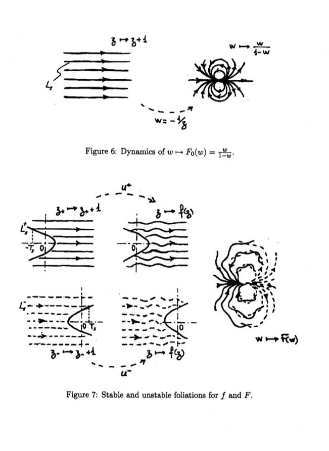
coordinates,thegerm$F$simply reads$z^{\pm}\mapsto z^{\pm}+1$ (see Figure 7), the complexityof the dynamics

being hiddenin the fact that neither $v^{+}$ nor $v^{-}$ is defined in a whole neighbourhood ofinfinity

and that these transformations do not coincide on the two connected componentsof $D^{+}\cap D^{-}$

(exceptof

course

if$F$and $F_{0}$ areanalytically$\mathrm{c}\mathrm{o}\mathrm{n}\mathrm{j}\mathrm{u}\mathrm{g}\mathrm{a}\mathrm{t}\mathrm{e}\mathrm{d}$)$-\mathrm{s}\mathrm{e}\mathrm{e}$ the noteattheend of this section

for a more “dynamical” and quickerconstruction of$v^{\pm}$.

This complexity can be analysed through the change of chart $v^{+}\mathrm{o}u^{-}=\mathrm{I}\mathrm{d}+\chi$, which is

a priori defined on $\mathcal{E}=D^{-}\cap(u^{-})^{-1}(D^{+})$; this set has an “upper” and a “lower” connected

components, $\mathcal{E}^{\mathrm{u}\mathrm{p}}$ and $\mathcal{E}^{1\mathrm{o}\mathrm{w}}$ (because

$(u^{-})^{-1}(D^{+})$ is a sectorial neighbourhood of infinity of

the same kind

as

$D^{+}$), and we thus get two analytic functions

$\chi^{\mathrm{u}\mathrm{p}}$ and $\chi^{1\mathrm{o}\mathrm{w}}$ (this situation

is reminiscent of the

one

described in Section 1.2). _{The conjugacy equations satisfied by} $u^{-}$

and $v^{+}$ yield_{$\chi(z+1)=\chi(z)$}, hence both

$\chi^{\mathrm{u}\mathrm{p}}$ and $\chi^{1\mathrm{o}\mathrm{w}}$

are

1-periodic; moreover, we

know that

these functions tend to $0$ as $\Im mzarrow\pm\infty$ (faster than any power of $z^{-1}$, by compovition of

asymptotic expansions). We thus get two Fourier series

$\chi^{1\mathrm{o}\mathrm{w}}(z)=v^{+}\circ u^{-}(z)-z=\sum_{m\geq 1}B_{m}\mathrm{e}^{-2\pi \mathrm{i}mz}$, $\Im mz<-\tau_{0}$, (24)

$\chi^{\mathrm{u}\mathrm{p}}(z)=v^{+}\mathrm{o}u^{-}(z)-z=\sum_{m\leq-1}B_{m}\mathrm{e}^{-2\pi \mathrm{i}mz}$, $\Im mz>\tau_{0}$, (25)

which are convergent for $\tau_{0}>0$ large enough. It turns out that the classification problemcan

be solved this way: two non-degenerate parabolic germs with vanishing resiter

are

analytically

conjugate

_if

and only

_if

they

_define

the

same

pair

_of

Fourierse$r\cdot ies(\chi^{\mathrm{u}\mathrm{p}}, \chi^{1\mathrm{o}\mathrm{w}})$up to a change

of

variable $zrightarrow z+c$; morevover, any pair

of

Fourier series

of

the type (24)_$-(25)$ can be obtained

this

way.11

The numbers $B_{m}$

are

said to be “analytic invariants” for the germ _$f$ or $F$

.

The

functions $\mathrm{I}\mathrm{d}+\chi^{1\mathrm{o}\mathrm{w}}$ and

$\mathrm{I}\mathrm{d}+\chi^{\mathrm{u}\mathrm{p}}$themselves

are

called “horn

maps.12

$1_{\mathrm{O}\mathrm{b}\mathrm{s}\mathrm{e}\mathrm{r}\mathrm{v}\mathrm{e}}$that,

when theparabolicgermattheorigin$F(w)\in w\mathbb{C}\{w\}$extendstoanentire function, the function

$U^{-}(z)=-1/u^{-}(z)$ _{also extends to} an_{entire function} _(because_the_{domain of}_analyticity$D^{-}$ contains the

half-plane$\Re ez<-\tau$_{and the relation}_{$U^{-}(z+1)=F(U^{-}(z))$} _allows_one_{to define the analytic continuation of}$U^{-}$ by

$U^{-}(z)=F^{\mathfrak{n}}(U^{-}(z-n))$,with$n\geq 1\mathrm{l}\mathrm{a}\mathrm{r}\mathrm{g}\mathrm{e}$enough foragiven

$z$),which$\mathrm{a}\mathrm{d}\mathrm{m}\mathrm{i}\mathrm{t}\mathrm{s}-1/\tilde{u}(z)=-z^{-1}(1+z^{-1}\tilde{\varphi}(z))^{-1}\in$

$z^{-1}\mathbb{C}[[z^{-1}]]$ asasymptoticexpansionin$D^{-}$. In this case, the formal series$\tilde{\varphi}(z)$must be divergent(if not, $-1/\tilde{\mathrm{u}}(z)$

would beconvergent, $U^{-}$ would beits sum and this entire function would have to be_constant), as_wellas $\tilde{\psi}(z)$,

and the Fatou coordinates $v^{+}$ and $v^{-}$ cannot be the analytic continuation one of the other. We have asimilar

situation when$F^{-1}(w)\in w\mathbb{C}\{w\}$ extends toan entire function,with _{$U^{+}(z)=-1/u^{+}(z)$}_entire.

11 _{For the first} _statement, _consider

$f_{1}$ and $f_{2}$ satisfying $\chi_{2}^{\mathrm{u}_{\mathrm{P}}}(z)=\chi_{1}^{\mathrm{u}\mathrm{p}}(z+c)$ and $\chi_{2}^{1\mathrm{w}}(z)=\chi_{1}^{1m}(z+c)$

with $c\in \mathbb{C}$, thus $v_{2}^{+}\mathrm{o}u_{2}^{-}=\tau^{-1}\mathrm{o}v_{1}^{+}\mathrm{o}u_{1}^{-}\mathrm{o}\tau$ in $\mathcal{E}^{\mathrm{u}\mathrm{p}}$ and $\mathcal{E}^{\mathrm{t}\mathrm{o}\mathrm{w}}$,

with $\tau(z)=z+c$. Using $(\tilde{u}_{1}0\tau, \tau^{-1}0\tilde{v}_{1})$

instead of$(\tilde{u}_{1},\tilde{v}_{1})$, we seethataformal conjugacy between$f_{1}$ and $f_{2}$is given by$\tilde{u}_{2}0\tau^{-1}0\tilde{v}_{1}$; its Borel-Laplace

sums $u_{2}^{+}\mathrm{o}\tau^{-1}\mathrm{o}v_{1}^{+}$ and $u_{2}^{-}\mathrm{o}\tau^{-1}\mathrm{o}v_{1}^{-}$ can be glued together and give rise to an analytic conjugacy, since $u_{2}^{-}=u_{2}^{+}\mathrm{o}\tau^{-1}\mathrm{o}v_{1}^{+}\circ u_{1}^{-}\mathrm{o}\tau$

.

Conversely, if there exists

$h\in \mathrm{I}\mathrm{d}+\mathbb{C}\{z^{-1}\}$suchthat$f_{2^{\mathrm{O}}}h=h\mathrm{o}f_{1}$, we seethat$h\mathrm{o}\tilde{u}_{1}$

establishesaformalconjugacybetween$f_{2}$ and $zrightarrow z+1$, Proposition 4 thus implies the existence of$c\in \mathbb{C}$ such

that$\tilde{u}_{2}=h\mathrm{o}\tilde{u}_{1}0\tau$and$\tilde{v}_{2}=\tau^{-}\mathrm{i}$$0\tilde{v}_{1}\mathrm{o}h^{-1}$,with_{$\tau(z)=z+C$},whence$u_{2}^{\pm}=h\mathrm{o}u_{1}^{\pm}\mathrm{o}\tau$ and$v_{2}^{\pm}=\tau^{-1}\mathrm{o}v_{1}^{\pm}\mathrm{o}h^{-1}$,

and$v_{2}^{+}\mathrm{o}u_{2}^{-}=\tau^{-1}\mathrm{o}v_{1}^{+}\mathrm{o}\mathrm{u}_{1}^{-}\mathrm{o}\tau$,asdesired. Theproofof the second statement is

beyondthe scope of thepresent

text.

12In fact, this name (which is ofA. Douady’s coinage) usually refers to the maps $\mathrm{I}\mathrm{d}+\chi^{1\mathrm{o}\mathrm{w}}$ expressed in the

coordinate $w_{-}=e^{-2\pi \mathrm{i}z},$ $i.e$

.

$w_{-} rightarrow w_{-}\exp(-2\pi \mathrm{i}\sum_{m\geq 1}B_{m}w_{-}^{m})$, and $\mathrm{I}\mathrm{d}+\chi^{\mathrm{u}\mathrm{p}}$ expressed in the coordinate

$w+=e^{2\pi \mathrm{i}z},$ $i.e$

.

$w+ rightarrow w+\exp(2\pi \mathrm{i}\sum_{m\geq 1}B_{-m}w_{+}^{m})$, which are holormophic for $|w\pm|<\mathrm{e}^{-2\pi\tau_{\mathrm{O}}}$ and can be

viewedas return maps; thevariables$w\pm \mathrm{a}\mathrm{r}\mathrm{e}$natural coordinates at both ends of“\’Ecalle’scylinder”. See[MR83],

Resurgent functions and splitting problems(New Trends and Applications of Complex Asymptotic Analysis : around dynamical systems, summability, continued fractions)

Resurgent

functions

and

splitting

problems

Sauzin

\’Ecalle’s

Contents

.

3

3

sums.

functions.

. .

6

.

.

.

.

.

.

.

.

.

. .

of

surface

. .

.

.

9

of

.

. .

.

.

.

.

.

.

10

difference

.

.

.

.

.

.

.

.

.

.

. .

of

foliation.

.

.

. .

functions.

.

\’Ecalle’s

.

. .

.

. .

.

.

of

of

.

.

.

.

. .

.

.

of

of

formal

₃

₃

_functions.

₆

_of

_surface

_of

_difference

_of

_foliation.

_functions.

_.

_of

_of

_of

_of

_formal

_transform.

_transfom

_of

_for

_of

_formd

_transform

₁