The Valuation of Callable Russian Options for Double Exponential Jump Diffusion Processes (Financial Modeling and Analysis)

The

Valuation

of

Callable Russian

Options for

Double

Exponential

Jump

Diffusion

Processes

南山大学・数理情報研究科, 数理情報研究センター 鈴木淳生1(Atsuo Suzuki)

Graduate School of Mathematical Sciences and Information Engineering

Nanzan University

南山大学・数理情報学部 澤木勝茂 (Katsushige Sawaki)

Faculty of Mathematical Sciences and Information Engineering

Nanzan University

Keywords: callable Russian Option, double exponential distribution,optimal stopping,

opti-mal boundaries

1. Introduction

Russian option was introduced by Shepp and Shiryaev [6], [7] and is

one

ofperpetual American lookback options. In Russian option the buyer has the right to exercise it at any time. On

the other hand, in callable Russian option not only the buyer but also the seller has the right

to cancel it at any time. This option is formulated as coupled optimal stopping problem. See

Cvitanic and Karatzas [1] Kifer [2].

Kyprianou [5] derived the closed-form solution in the

case

where the dividend rate is

zero.

Suzuki and Sawaki [8] gave the pricing formula with positive dividend. Kou andWang [4]

gave

the

closed form

for

the value

function ofperpetual

American

put options without

dividend

and

so

on.

Suzuki and Sawaki [9] derived the pricing formula of non-callable Russian option for

double exponentialjump diffusion processes.

In this paper,

we

deal with callable Russian options. A callable Russian option is

a

contact

that the seller and the buyer have the rights to cancel and to exercise at anytime, respectively.

Wepresent thepricing formula of callable Russianoptionsfor double exponential jump diffusion

processes. The pricing of such

an

option

can

be formulated

as

a coupled optimal stopping

problemwhich is analyzed

as

Dynkin game. We derive the value function of

a

callable Russian

option and its optimal boundaries. Also

some

numerical results

are

presented to demonstrate

analytical sensitives of the value function with respect to parameters.

This paper is organized

as

follows. In section 2

we

introduce

a

pricing model of callable Russian options by lneans of a coupled optimal stopping problem given by Kifer [2]. Section

3 presents the value function of callable Russian options for double exponential jump diffusion

processes. Section 4 presents numerical examples to verify analytical results. We end the paper

with

some

concluding remarks and future work.

2. Pricing model

In this section

we

consider the pricing model for the callable Russian option. Let $B(t)$ be the process of the riskless asset price at time $t$ defined by $B(t)=B(())e^{rt}$, where $r$ is positive

interest rate. Let $W(t)$ be astandard Brownian motion and $N(t)$ be aPoisson process with the

intensity $\lambda$

.

Let

$J_{i}$ denote i.i.$d$

.

positive random variables. $Y_{l}\equiv\log J_{i}$ has a double exponential

distribution and its the density function is given by

$f(y)=p\eta_{1}e^{-\eta_{1}y}1_{tv\geq 0\}}+q\eta_{2}e^{\eta_{2}y}1_{\{y<0\}}$,

where $\eta_{1}>1,$ $\eta_{2}>0$ and $0\leq p,$$q\leq 1$ such that$p+q=1$

.

Under a risk-neutral probability, the

process of the risky asset price $S(t)$ at time $t$ satisfies the stochastic differential equation

$\frac{dS(t)}{S(t-)}=\mu dt+\kappa dW(t)+d(\sum_{i=1}^{N(t)}(J_{i}-1))$, (2.1)

where $\mu$ and $\kappa>0$ are constants. Define another probability

measure

$\tilde{P}$

as

$\frac{d\tilde{P}}{dP}|_{F\ell}=\exp\{-bW(t)-\frac{1}{2}b^{2}t\},$ $b= \frac{\mu-r+d+\lambda\zeta}{\kappa}$,

where $d$ is the positive continuous dividend rate of the risky asset, _{$\mathcal{F}_{t}=\sigma(W^{r}(s), N(s),$$\{J_{i}\}$})

and

$\zeta=E[J_{i}]-1=\frac{p\eta_{1}}{\eta_{1}-1}+\frac{q\eta_{2}}{\eta_{2}+1}-1$

.

By Girsanov’s theorem, $\tilde{W}(t)=W(t)-bt$ is

a

Brownian motion with respect to $\tilde{P}$.

We

can

rewrite (2.1)

as

$\frac{dS(t)}{S(t-)}=(r-d-\lambda\zeta)dt+\kappa d\tilde{W}(t)+d(\sum_{i=1}^{N(t)}(J_{i}-1))$. (2.2)

Solving (2.2) gives $S(t)=S(O)$exp$X(t)$, where

$X(t)=(r-d- \frac{1}{2}\kappa^{2}-\lambda\zeta)t+\kappa\tilde{W}(t)+\sum_{i=1}^{N(t)}Y_{i}$

.

Let $V(v)$ be

a

function of class $C^{2}$

.

Then the infinitesimal generator $\mathcal{L}$ of the process $S(t)$ is

given by

$\mathcal{L}V(v)=\frac{1}{2}\kappa^{2}v^{2}V’’(v)+(r-d-\lambda\zeta)vV’(v)+\lambda.\int_{-\infty}^{\infty}(V(ve^{y})-V(v))f(y)dy$

for all $v>0$

.

Next we introduce the four real numbers $\beta_{1},$$\beta_{2},$$\beta_{3},$$\beta_{4}$

.

Kou and Wang (2003) showed that

the equation $G(\theta)=\alpha$ for all $\alpha>0$ has the solutions $\beta_{1},$ $\beta_{2},$$-\beta_{3},$ $-\beta_{4}$, where

$G( \theta)=\theta(r-d-\frac{1}{2}\kappa^{2}-\lambda\zeta)+\frac{1}{2}\theta^{2}\kappa^{2}+\lambda(\frac{p\eta_{1}}{\eta_{1}-\theta}+\frac{q\eta_{2}}{\eta_{2}+\theta}-1)$

And the four solutions satisfy

$0<\beta_{1}<\eta_{1}<\beta_{2}<\infty$, $0<\beta_{3}<\eta_{2}<\beta_{4}<\infty$.

Define the process

$\Psi(t)\equiv\max(vs,\sup_{0\leq u\leq t}S(u))/S(t)$, $S(0)=s,$$v\geq 1$

.

Then the value function of non-callable Russian options is given by

$V_{R}(v)= \sup_{\tau}\tilde{E}[e^{-r\tau}\Psi(\tau)|\Psi(0)=v]$,

where the supremum _{is taken for all stopping times} $\tau$

.

Theorem 2.1.

(Suzuki and Sawaki $[9J$) The value

function

$V(v)$

of

Russian option is given by

$V_{R}(v)=\{\begin{array}{ll}A(v_{1})v^{\beta_{1}}+B(v_{1})v^{\beta_{2}}+C(v_{1})v^{-\beta_{3}}+D(v_{1})v^{-\beta_{4}}, 1\leq v\leq v_{1}v, v\geq v_{1}.\end{array}$

The

_coefficients

are

determined by

$A(v_{1})$ $=$ $\frac{(\eta_{1}-\beta_{1})v_{1}^{-\beta_{1}}}{(\beta_{1}+\beta_{3})(\beta_{2}-\beta_{1})}\{\frac{(\mathcal{B}_{2}-1)(\beta_{3}+1)}{\eta_{1}-1}v_{1}-\frac{(\beta_{2}+\beta_{4})(\beta_{4}-\beta_{3})}{\eta_{1}+\beta_{4}}Dv_{1}^{-\beta_{4}}\}$

$B(v_{1})$ $=$ $\frac{(\beta_{2}-\eta_{1})v_{1}^{-\beta_{2}}}{(\beta_{2}-\beta_{1})(\beta_{2}+\beta_{3})}\{\frac{(\beta_{1}-1)(\beta_{3}+1)}{\eta_{1}-1}v_{1}-\frac{(\beta_{1}+\beta_{4})(\beta_{4}-\beta_{3})}{\eta_{1}+\beta_{4}}Dv_{1}^{-\beta_{4}}\}$

$C_{\text{ノ}}(v_{1})$ $=$ $\frac{(\eta_{1}+\beta_{3})v_{1}^{\beta_{3}}}{(\beta_{1}+\beta_{3})(\beta_{2}+\beta_{3})}\{\frac{(\beta_{1}-1)(\beta_{2}-1)}{\eta_{1}-1}v_{1}-\frac{(\beta_{1}+\beta_{4})(\beta_{2}+\beta_{4})}{\eta_{1}+\beta_{4}}Dv_{1}^{-\beta_{4}}\}$

and

$\frac{A(v_{1})}{\eta_{2}+\beta_{1}}+\frac{B(v_{1})}{\eta_{2}+\beta_{2}}+\frac{C(v_{1})}{\eta_{2}-\beta_{3}}+\frac{D(v_{1})}{\eta_{2}-\beta_{4}}$ _$=$ $0$

.

Moreover, the optimal $bounda\eta v_{1}$ is the solution in $(1, \infty)$ to the equation

$A(v)\beta_{1}+B(v)\beta_{2}-C(v)\beta_{3}-D(v)\beta_{4}=0$

and the optimal stopping time is given by

$\hat{\tau}=\inf\{t>0|\Psi(t)\geq v_{1}\}$.

3.

Callable Russian

options

We

assume

that $p=1$ and $q=0$

.

It

means

_{that the jump is down only. Then}

we

_can

_express

$G(\theta)$

as

$G( \theta)=\theta(r-d-\frac{1}{2}\kappa^{2}-\lambda\zeta)+\frac{1}{2}\theta^{2}\kappa^{2}+\lambda(\frac{\eta_{1}}{\eta_{1}-\theta}-1)$

and the equation $G(\theta)=r$ has three solutions $\beta_{1},$$\beta_{2},$$-\beta_{4}$, which satisfy

$1\leq\beta_{1}<\eta_{1}<\beta_{2}<\infty$, $0<\beta_{4}<\infty$

.

Let $\sigma$denote

a

cancel time fortheseller and

$\tau$

an

exercise timeforthe buyer. If the seller cancels

the contract, the buyer receives $\Psi(\sigma)\neq\delta$ from the seller. We can think of $\delta>0$

as

the penalty

cost for the cancel. On the other hand, if the buyer exercises it, (s)he receives $\Psi(\tau)$ from the

seller. Therefore, the payoff function ls given by

Let $\mathcal{T}_{0,\infty}$ denote the set of all stopping times with values in the interval _{$[0, \infty]$}

.

Then the value

function $V^{*}(v)$ of the callable Russian option is defined by

$V^{*}(v)=$ inf $supJ(\sigma, \tau, v)$, (3.1)

$\sigma\in \mathcal{T}_{0,\infty\tau\in \mathcal{T}_{0,\infty}}$

where

$J(\sigma, \tau, v)=\tilde{E}[e^{-\alpha(\sigma\wedge\tau)}\{(\Psi(\sigma)+\delta)1_{\{\sigma<\tau\}}+\Psi(\tau)1_{\{\tau\leq\sigma\}}\}|\Psi(0)=v]$

.

And the function $V^{*}(v)$ satisfies the inequalities

$v\leq V^{*}(v)\leq v+\delta$,

which provides the lower and the upper bounds for the value function of the callable Russian

option.

We

define

two sets $A$ and $B$

as

$A$ $=$ $\{v\in R^{+}|V(v)=v+\delta\}$

$B$ $=$ $\{v\in R^{+}|V(v)=v\}$

.

$A$ and $B$

are

called the seller’s cancel region and the buyer’s exercise region, respectively. Then

the two optimal stopping times are given by

$\sigma_{A}$ $=$ $\inf\{t>0|\Psi(t)\in A\}$,

$\tau_{B}$ $=$ $\inf\{t>0|\Psi(t)\in B\}$

.

Then for any$v,\hat{\sigma}\equiv\sigma_{A}$ and $\hat{\tau}\equiv\tau_{B}$ attain the infimum and supremumin (3.1), _$i.e.$, we have

$V^{*}(v)=J(\hat{\sigma},\hat{\tau}, v)$

.

The pair $(\hat{\sigma},\hat{\tau})$ is the saddle point of $J(\sigma, \tau, v)$

.

Remark 3.1. The

seller

minimizes the payofffunction and$\Psi(t)\geq\Psi(O)=v\geq 1$

.

$fi$}_$vm$ this, $it$

follows

that the seller’s optimal cancel $r_{\mathfrak{B}^{ion}}$ is

{1}.

Lemma

3.1.

Suppose that$r-d- \frac{1}{2}\kappa^{2}-\lambda\zeta>0$

.

Then the

function

$V(v)$ is Lipschitz continuous

and its Radon-Nikodym dertvative

_satisfies

$0\leq V’(v)\leq 1$, $a.e$

.

$v$

.

(3.2)

Proof.

Since $\hat{\sigma},\hat{\tau}$ and _$\Psi(t)$ depends

on

the initial value

$v$,

we

write them

as

$\hat{\sigma}^{v},\hat{\tau}^{v}$ and _{$\Psi(t, v)$}

.

Replacing the optimal stopping times $\hat{r}^{v}$ by another stopping time $\hat{\tau}^{u}$, we get the inequalities

$V(v)\leq J(\hat{\sigma}^{u},\hat{\tau}^{v}, v)$

,

$V(u)\geq J(\hat{\sigma}^{u},\hat{\tau}^{v}, u)$

.

Note that $z_{1}^{+}-z_{2}^{+}\leq(z_{1}-z_{2})^{+}$ for any $z_{1},$$z_{2}\in R$

.

For any $v\geq u$,

we

have

$0$ $\leq$ $V(v)-V(u)$

$=$ $J(\hat{\sigma}^{u},\hat{\tau}^{v},v)-J(\hat{\sigma}^{u},\hat{\tau}^{v}, u)$

$=$ $\tilde{E}[e^{-\alpha}’\wedge\hat{\tau}^{\prime J})(\Psi(\hat{\sigma}^{u}\wedge\hat{\tau}^{v},v)-\Psi(\hat{\sigma}^{14}\wedge\hat{\tau}^{v},u))]$ $=$ $\tilde{E}$

[$e^{-\alpha(\hat{\sigma}^{u}\wedge\hat{\tau}^{v})}H^{-1}$($\hat{\sigma}^{u}$ A$\hat{\tau}^{v}$)

$\{(v$ –$supH_{u})^{+}-(u$-$supH_{u})^{+}\}$]

$\leq$ $(v-u)\tilde{E}[e^{-\alpha(\dot{\sigma}^{u}\wedge f)}H^{-1}(\hat{\sigma}^{u}\wedge\hat{\tau}^{v})]$

$\leq$ $v-u$,

where $H(t)=\exp X(t)$

.

Therefore,

_we

_obtain

$0 \leq\frac{V(v)-V(u)}{c1-\prime u}\leq 1$

.

If the penalty $\delta$ is too large, the seller never

cancels. How large $\delta$ is it?

Lemma 3.2. Set$\delta^{*}=V_{R}(1)-1$.

If

thepenalty$\delta>\delta^{*}$, the sellernever cancels. In otherwords,

the callable Russian option is reduced to Russian option.

Proof.

Consider thefunction $U(v)=V_{R}.(v)-v-\delta$

.

Since it holds $U’(v)\leq 0$ by Lemma 3.1 and

$U(1)=\delta^{*}-\delta<0$,

we

have $V_{R}(v)<v+\delta$

.

Hence, it follows that $V^{*}(v)<v+\delta$ because it holds

that $V(v)\leq V_{R}(v)$

.

_口

We introduce the function for $v_{0}=e^{x_{0}}>1$

$V(v)=\{\begin{array}{ll}A_{v^{\beta_{1}}}+Bv^{\beta_{2}}+Cv^{-\beta_{4}}, 1\leq v\leq v_{0}v, v\geq v_{0}.\end{array}$ (3.3)

We set $v=e^{x}$ and $V(v)=V(e^{x})\equiv t^{V}(x)\wedge$

.

In what follows,

we

determine the

coefficients

$A,$$B,$$C$

and $e^{xo}$

.

In order to determine the coefficients,

we

prepare the conditions. By value matching

condition,

we

have

$Ae^{\beta_{1}x0}+Be^{\beta_{2}xo}+Ce^{-\beta_{4}x0}=e^{x0}$

and by smooth pasting condition,

we

have

$A\beta_{1}e^{\beta_{1}x_{0}}\neq B\beta_{2}e^{\beta_{2}x_{0}}-C\beta_{4}e^{-\beta_{4}x_{0}}=e^{x0}$

.

We

can

get the last condition by using the infinitesimal generator $\hat{\mathcal{L}}$

ofthe process $X(t)$ given by

$\hat{\mathcal{L}}\hat{V}(x)=\frac{1}{2}\kappa^{2}\hat{V}’’(x)+(r-d-\frac{1}{2}\kappa^{2}-\lambda\zeta)\hat{V}’(x)+\lambda\int_{-\infty}^{\infty}(\hat{V}(x+y)-\hat{V}(x))f(y)dy$

for all $v>0$

.

For $x<x_{0}$, we obtain

$/-\infty\infty\hat{V}(x+y)f(y)dy$

$=$ $\int_{0}^{x0-x}(Ae^{\beta_{1}(x\neq y)}+Be^{\beta_{2}(x+y)}+Ce^{-\beta_{4}(x+y)})\eta_{1}e^{-\eta_{1}y}dy+\int_{x_{0}-x}^{\infty}e^{x+y}\eta_{1}e^{-\eta_{1}y}dy$

$=$ $\eta_{1}(\frac{A}{\eta_{1}-\beta_{1}}e^{\beta_{1}x}+\frac{B}{\eta_{1}-\beta_{2}}e^{\beta_{2}x}+\frac{C}{\eta_{1}+\beta_{4}}e^{-\beta_{4}x})$

$- \eta_{1}e^{-\eta_{1}(x_{0}-x)}(\frac{A}{\eta_{1}-\beta_{1}}e^{\beta_{1}x_{0}}+\frac{B}{\eta_{1}-\beta_{2}}e^{\beta_{2}x_{0}}+\frac{C}{\eta_{1}+\beta_{4}}e^{-\beta_{4}x_{0}}-\frac{e^{x0}}{\eta_{1}-1})$

.

IFlrom this,

we

obtain

$(\hat{L}-r)\hat{V}(x)$ $=$ $Ae^{\beta_{1}x}( \frac{1}{2}\beta_{1}^{2}+\beta_{1}(r-d-\frac{1}{2}\kappa^{2}-\lambda\zeta))+Be^{\beta_{2}x}(\frac{1}{2}\beta_{2}^{2}+\beta_{2}(r-d-\frac{1}{2}\kappa^{2}-\lambda\zeta))$ $+Ce^{-\beta_{4}x}( \frac{1}{2}(-\beta_{4})^{2}-\beta_{4}(r-d-\frac{1}{2}\kappa^{2}-\lambda\zeta))$ $+ \lambda.\int_{-\infty}^{\infty}\nu^{r}(x+y)f(y)dy-(\lambda+r)\hat{V}(x)$ ’ $=$ $Ae^{\beta_{1}x}g(\beta_{1})+Be^{\beta_{2}x}g(\beta_{2})+Ce^{-\beta_{4}x}g(-\beta_{4})$ $- \lambda p\eta_{1}e^{-\eta_{1}(x0-x)}(\frac{A}{\eta_{1}-\beta_{1}}e^{\beta_{1}x_{0}}+\frac{B}{\eta_{1}-\beta_{2}}e^{\beta_{2}xo}+\frac{C}{\eta_{1}+\beta_{4}}e^{-\beta_{4}xo}-\frac{e^{x_{0}}}{\eta_{1}-1})$,

where

$g(x)=G(-x)-r$

.

By Lemma 2.1 in Kou and Wang [3], wehave$g(\beta_{1})=g(\beta_{2})=9(\beta_{4})=$

$0$. Since $(\hat{\mathcal{L}}-r)\hat{V}(x)=0$ holds, we get the condition

$\frac{A}{\eta_{1}-\beta_{1}}e^{\beta_{1}x0}+\frac{B}{\eta_{1}-\beta_{2}}e^{\beta_{2}x_{0}}+\frac{C}{\eta_{1}+\beta_{4}}e^{-\beta_{4}x_{0}}-\frac{e^{xo}}{\eta_{1}-1}=0$

.

(3.4)

Lemma 3.3. Solving thefollowing equations

$Ae^{\beta_{1}x0}+Be^{\beta_{2}x_{0}}+Ce^{-\beta_{4}x0}$ _$=$ $e^{x_{0}}$

$A\beta_{1}e^{\beta_{1}x_{0}}+B\beta_{2}e^{\beta_{2}x_{0}}-C\beta_{4}e^{-\beta_{4}x0}$ _$=$ $e^{x_{0}}$

$\frac{A}{\eta_{1}-\beta_{1}}e^{\beta_{1}x_{0}}+\frac{B}{\eta_{1}-\beta_{2}}e^{\beta_{2}x_{0}}+\frac{C}{\eta_{1}+\beta_{4}}e^{-\beta_{4}xo}$ $=$ $\frac{e^{x_{0}}}{\eta_{1}-1}$

gives the solutions

$A$ $=$ $\frac{(\eta_{1}-\beta_{1})(\beta_{2}-1)(\beta_{4}+1)}{(\eta_{1}-1)(\beta_{1}+\beta_{4})(\beta_{2}-\beta_{1})}e^{(1-\beta_{1})x_{0}}$

$B$ $=$ $\frac{(\beta_{2}-\eta_{1})(\beta_{1}-1)(\beta_{4}+1)}{(\eta_{1}-1)(\beta_{2}+\beta_{4})(\beta_{2}-\beta_{1})}e^{(1-\beta_{2})x_{0}}$

$C$ $=$ $\frac{(\eta_{1}+\beta_{4})(\beta_{2}-1)(\beta_{1}-1)}{(\eta_{1}-1)(\beta_{1}+\beta_{4})(\beta_{2}+\beta_{4})}e^{(1+\beta_{4})x_{0}}$

.

Since thecoefficients $A,$$B,$$C$depend

on

$x_{0}$,

we

denote them

as

$A(x_{0}),$ $B(x_{0})$ and$C(x_{0})$

.

The

number $v0=e^{x_{0}}$ given by (3.3) satisfies the equation

$A(x_{0})e^{\beta_{1}x0}+B(x_{0})e^{\beta_{2}x_{0}}\cdot+C(x_{0})e^{-\beta_{4}x_{0}}=\delta+1$

.

In the remainder of this section,

we

discuss the

case

where$p,$$q>0$

.

We set

a

function $V(v)$

$V(v)=\{\begin{array}{ll}Av^{\beta_{1}}+Bv^{\beta_{2}}+Cv^{-\beta_{\delta}}+Dv^{-\beta_{4}}, 1\leq v\leq v_{0}v, v\geq v_{0}.\end{array}$

By value matching condition

and

smooth pasting condition,

we

have

$Ae^{\beta_{1}x0}+Be^{\beta_{2}x0}+Ce^{-\beta sx_{0}}+De^{-\beta_{4}x0}$ _$=$ $e^{x0}$

$A\beta_{1}e^{\beta_{1}x_{0}}+B\beta_{2}e^{\beta_{2}x_{0}}-C\beta_{3}e^{-\beta\prime sx_{0}}-D\beta_{4}e^{-\beta_{4}x0}$ _$=$ $e^{x0}$,

respectively. For $x_{1}<x<x_{0}$, wehave

$1_{-\infty}^{\infty}\hat{V}(x+y)f(y)dy$ $=$ $\int_{x_{1}-x}^{0}(Ae^{\beta_{1}(x+y)}+Be^{\beta_{2}(x+y)}+Ce^{-\beta s(x+y)}+De^{-\beta_{4}(x+y)})q\eta_{2}e^{\eta_{2}y}dy$ $+.1_{0}^{x0-x}(Ae^{\beta_{1}(x+y)}+Be^{\beta_{2}(x+y)}+c_{e^{}}^{-\beta_{3}(x+y)}+De^{-\beta_{4}(x+y)})p\eta_{1}e^{-\eta_{1}y}dy$ $+ \int_{x0-x}^{\infty}e^{x+y}p\eta_{1}e^{-\eta_{1}y}dy$ $=$ $q \eta_{2}(\frac{A}{\eta_{2}+\beta_{1}}e^{\beta_{1}x}+\frac{B}{\eta_{2}\dashv-\beta_{2}}e^{\beta_{2}x}+\frac{C}{\eta_{2}-\beta_{3}}e^{-d_{3}x}+\frac{D}{\eta_{2}-\beta_{4}}e^{-\beta_{4}x})$ $-q \eta_{2}e^{r\rho(x_{1}-x)}(\frac{A}{\eta_{2}+\beta_{1}}e^{\beta_{1}x_{1}}+\frac{B}{7|2+\beta_{2}}e^{r_{i_{2}x_{1}}}+\frac{C}{\eta_{2}-l?_{3}}e^{--\beta_{3}x_{1}}+\frac{D}{\eta_{2}-\beta_{4}}e^{-\beta_{4}x_{1}})$

$+p \eta_{1}(\frac{A}{\eta_{1}-\beta_{1}}e^{\beta_{1}x\beta_{2}x-\beta_{d}x\beta_{4}x)}+\frac{B}{\eta_{1}-\beta_{2}}e+\frac{C}{\eta_{1}+\beta_{3}}e+\frac{D}{\eta_{1}+\beta_{4}}e^{-}$ $-p \eta_{1}e^{-\eta_{1}(x_{0}-x)}(\frac{A}{\eta_{1}-\beta_{1}}e^{\beta_{1}x0}+\frac{B}{\eta_{1}-\beta_{2}}e^{\beta_{2}x_{0}}+\frac{C}{\eta_{1}+\beta_{3}}e^{-\beta sxo}+\frac{D}{\eta_{1}+\beta_{4}}e^{-\beta_{4}x_{0}})$ $+p\eta_{1}e^{-\eta_{1}(x_{0}-x)_{\frac{e^{x_{0}}}{\eta_{1}-1}}}$. Therefore,

we

obtain $(\hat{L}-r)\hat{V}(x)$ $=$ $Ae^{\beta_{1}x}( \frac{1}{2}\beta_{1}^{2}+(r-d-\frac{1}{2}\kappa^{2}-\lambda\zeta)\beta_{1})$ $+Be^{\beta_{2}x}( \frac{1}{2}\beta_{2}^{2}+(r-d-\frac{1}{2}\kappa^{2}-\lambda\zeta)\beta_{2})$ $+Ce^{-\beta_{3}x}( \frac{1}{2}(-\beta_{3})^{2}+(r-d-\frac{1}{2}\kappa^{2}-\lambda\zeta)(-\beta_{3}))$ $+De^{-\beta_{4}x}( \frac{1}{2}(-\beta_{4})^{2}+(r-d-\frac{1}{2}\kappa^{2}-\lambda\zeta)(-\beta_{4}))$ $+ \lambda\int_{-\infty}^{\infty}\hat{V}(x+y)f(y)dy-(\lambda+r)\hat{V}(x)$ $=$ $Ae^{\beta_{1}x}g(\beta_{1})+Be^{\beta_{2}x}g(\beta_{2})+Ce^{-\beta_{3}x}g(-\beta_{3})+De^{-\beta_{4}x}g(-\beta_{4})$ $- \lambda p\eta_{1}e^{-\eta_{1}(x0-x)}(\frac{Ae^{\beta_{1}x_{0}}}{\eta_{1}-\beta_{1}}+\frac{Be^{\beta_{2}x_{0}}}{\eta_{1}-\beta_{2}}+\frac{Ce^{-\beta_{3}x_{0}}}{\eta_{1}+\beta_{3}}+\frac{De^{-\beta_{4}x0}\prime}{\eta_{1}+\beta_{4}}-\frac{e^{x_{0}}}{\eta_{1}-1})$ $- \lambda q\eta_{2}e^{\eta_{2}(x_{1}-x)}(\frac{Ae^{\beta_{1}x_{1}}}{\eta_{2}+\beta_{1}}+\frac{Be^{\beta_{2}x_{1}}}{\eta_{2}+\beta_{2}}+\frac{Ce^{-\beta_{3}x_{1}}}{\eta_{2}-\beta_{3}}+\frac{De^{-\beta_{4}x_{1}}}{\eta_{2}-\beta_{4}}I\cdot$

Since

$(\hat{\mathcal{L}}-r)\hat{V}(x)=0$ for

$x_{1}<x<x_{0}$ ,

we can

get

$\frac{A}{\eta_{1}-\beta_{1}}e^{\beta_{1}x_{0}}+\frac{B}{\eta_{1}-\beta_{2}}e^{\beta_{2}x0}+\frac{C}{\eta_{1}+\beta_{3}}e^{-\beta_{3}x0}+\frac{D}{\eta_{1}+\beta_{4}}e^{-\beta_{4}x_{0}}-\frac{e^{x_{0}}}{\eta_{1}-1}$ $=$ $0$

$\frac{A}{\eta_{2}+\beta_{1}}e^{\beta_{1}x_{1}}+\frac{B}{\eta_{2}+\beta_{2}}e^{\beta_{2}x_{1}}+\frac{C}{\eta_{2}-\beta_{3}}e^{-\beta_{3}x_{1}}+\frac{D}{\eta_{2}-\beta_{4}}e^{-\beta_{4}x_{1}}$ $=$ $0$.

Lemma 3.4. Solving the equations yields

$Ae^{\beta_{1}x_{0}}+Be^{\beta_{2}x_{0}}+Ce^{-\beta_{3}x0}+De^{-\beta_{4}x_{0}}$ _$=$ $e^{x_{0}}$

$A\beta_{1}e^{\beta_{1}x0}+B\beta_{2}e^{\beta_{2}x0}-C\beta_{3}e^{-\beta_{3}x0}-D\beta_{4}e^{-\beta_{4}x0}$ _$=$ $e^{x_{0}}$

$\frac{A}{\eta_{1}-\beta_{1}}e^{\beta_{1}xo}+\frac{B}{7\prime 1-\beta_{2}}e^{\beta_{2}x_{0}}+\frac{C}{\eta_{1}+\beta_{3}}e^{-\beta_{3}x_{0}}+\frac{D}{\eta_{1}+\beta_{4}}e^{-\beta_{4}x0}$ $=$ $\frac{e^{x0}}{\eta_{1}-1}$

the solutions

$A$ $=$ $\frac{(\eta_{1}-\beta_{1})e^{-\beta_{1}x_{0}}}{(\beta_{1}+\beta_{3})(\beta_{2}-\beta_{1})}\{\frac{(\beta_{2}-1)(\beta_{3}+1)}{\eta_{1}-1}e^{x_{0}}-\frac{(\beta_{2}+\beta_{4})(\beta_{4}-\beta_{3})}{\eta_{1}+\beta_{4}}De^{-\beta_{4}x_{0}}\}$

$B$ $=$ $\frac{(\beta_{2}-\eta_{1})e^{-\beta_{2}x_{0}}}{(\beta_{2}-\beta_{1})(\beta_{2}+\beta_{3})}\{\frac{(\beta_{1}-1)(\beta_{3}+1)}{\eta_{1}-1}e^{x0}-\frac{(\beta_{1}+\beta_{4})(\beta_{4}-\beta_{3})}{\eta_{1}+\beta_{4}}De^{-\beta_{4}x_{0}}\}$

$C$ $=$ $\frac{(\eta_{1}+\beta_{3})e^{\theta_{3}x_{0}}}{(\beta_{1}+\beta_{3})(\beta_{2}+\beta_{3})}\{\frac{(\beta_{1}-1)_{(}’\beta_{2}-1)}{\eta_{1}-1}e^{x0}-\frac{(\beta_{1}+\beta_{4})(\beta_{2}+\beta_{4})}{\eta_{1}+\beta_{4}}De^{-\beta_{4}xo}\}$

.

And the solutions

_of

the equations

$\frac{A}{\eta_{2}+\beta_{1}}e^{\beta_{1}x_{1}}+\frac{B}{\eta_{2}+\beta_{2}}e^{\beta_{2}x_{1}}+\frac{C}{7|2-\beta_{3}}e^{-\beta_{3}x_{1}}+\frac{D}{\eta_{2}-\beta_{4}}e^{-\beta_{4}x_{1}}$ $=$ $0$

are given by

$A$ $=$ $- \frac{\eta_{2}+\beta_{1}}{\beta_{2}-\beta_{1}}\{\frac{\beta_{2}+\beta_{3}}{\eta_{2}-\beta_{3}}C+\frac{\beta_{2}+\beta_{4}}{\eta_{2}-\beta_{4}}D+\delta+1\}$

$B$ $=$ $\frac{\eta_{2}+\beta_{2}}{\beta_{2}-\beta_{1}}\{\frac{\beta_{1}+\beta_{3}}{\eta_{2}-\beta_{3}}C+\frac{\beta_{1}+\beta_{4}}{\eta_{2}-\beta_{4}}D+\delta+1\}$

.

By the above lemma,

we can

determinethe coefficients $A,$$B,$$C,$ $D$ and $v0$

.

4. Main Theorem

In this section

we

give the main theorem. In order to prove it,

we

needs the following lemmas.

Lemma 4.1. Assume that a

_function

$V(v)$ has the following$p$roperties.

1. $(\mathcal{L}-r)V(v)\leq 0$

,

for

_{$v>v_{0}$}

.

2.

It holds $(\mathcal{L}-r)V(v)=0$ and $V(x)$

satisfies

_{$v<V(v)<v+\delta$}

for

_{$1<v<v_{0}$}

.

3. At $v=\cdot v_{0}$

we

have $V’(v_{0}-)=V’(v_{0}+)$

.

Then, $V$ is the value

function

of

callable Russian options with dividend, i.e., _$V^{*}=V$ holds. The

optimal exercise region is the interval $[v_{0}, \infty$) and the optimal

can

cel region is

{1}.

In what follows

we

will explore the properties of the function $V(v)$ in Lemma 4,1.

Lemma 4.2. For$v>v_{0}$ the

function

$V(v)$

satisfies

$(\mathcal{L}-r)V(v)\leq 0$

.

Proof.

Since $\hat{V}(x)=e^{x}$ for _{$x>x_{0}$},

we

have

$\int_{0}^{\infty}\hat{V}(x+y)f(y)dy=\int_{0}^{\infty}\eta_{1}e^{x+(1-\eta_{1})y}dy=\frac{\eta_{1}e^{x}}{\eta_{1}-1}$

.

Hence, we obtain

$(\hat{\mathcal{L}}-r)\hat{V}(x)$ _{$=$ $\frac{1}{2}\kappa^{2}e^{x}+(r-d-\frac{1}{2}\kappa^{2}-\lambda\zeta)e^{x}+\frac{\lambda\eta_{1}}{\eta_{1}-1}e^{x}-(\lambda+r)e^{x}$}

$=$ $-de^{x}<0$.

That is, it holds $(\mathcal{L}-r)V(v)\leq 0$

.

_口

Lemma 4.3. For $1<v<v_{0}$ the

function

$V(v)$

satisfies

$(\mathcal{L}-r)V(v)=0$ and

$v<V(v)<v+\delta$

.

Proof.

The former assertion is known. We will show the latter

one.

The second derivative

of $V(v)$ is nonnegative because $\beta_{1},$_{$\beta_{2}>1$} and $A,$$B,$$C>0$

.

It follows that $V$ is

a

convex

function. Since $V(v)$ is

a convex

function, $V’(v)$ is increasing. From this,

we

can see

that

$V’(v)<1$ for $1<v<v_{0}$

.

By the boundary conditions $V(1)=\delta+1$ and $V(v_{0})=v_{0}$,

we

have

$v<V(v)<\tau)+\delta$

.

$\square$

Lemma 4.4. Set

$h(v)=\delta+1-A(v)v^{\beta_{1}}-B(v)v^{\beta_{2}}-C(.v)v^{-\theta_{4}}$

.

(4.1)

Proof.

By (4.1), a direct computation yields

$h(1)$ $=$ $\delta+1$

$(\eta_{1}-\beta_{1})(\beta_{2}-1)(\beta_{4}+1)$ $(\beta_{2}-\eta_{1})(\beta_{1}-1)(\beta_{4}+1)$ $(\eta_{1}+\beta_{4})(\beta_{2}-1)(\beta_{1}-1)$

$\overline{(\eta_{1}-1)(\beta_{1}+\beta_{4})(\beta_{2}-\beta_{1})}\overline{(\eta_{1}-1)(\beta_{2}+\beta_{4})(\beta_{2}-\beta_{1})}\overline{(\eta_{1}-1)(\beta_{1}+\beta_{4})(\beta_{2}+\beta_{4})}--$

$=$ $\delta>0$

.

Furthermore, Since $h(\infty)=-\infty,$$h”(v)<0$and _$h’(1)=0$, the equation _$h(v)=0$ has the unique

solution in $(1, \infty)$

.

$\square$

Theorem 4.1. Let $V^{*}(v)$ denote the value

function of

the callable Russian option.

If

$\delta\geq\delta^{*}$,

the value

_function

is equal to non-callable Russian option, i.e. $V^{*}(v)=V_{R}(v)$

.

If

$\delta<\delta_{*}$

,

then

$V^{*}(v)$ is given by

$V(v)=\{\begin{array}{l}A(v_{0})v^{\beta_{1}}+B(v_{0})v^{\beta_{2}}+C(v_{0})v^{-\beta_{4}}1\leq v\leq v_{0}vv\geq v_{0}\end{array}$

and the optimal stopping times are given by

$\hat{\sigma}$

$=$ $\inf\{t>0|\Psi(t)=1\}$,

$\hat{\tau}$

$=$ $\inf\{t>0|\Psi(t)\geq vo\}$

.

The optimal boundary $v_{0}$

for

the buyer is the unique solution to the equation

$A(v)v^{\beta_{1}}+B(v)v^{\beta_{2}}+C(x_{0})v^{-\beta_{4}}=\delta+1$

.

Moreover, the

_function

$V(v)$ is also represented by

$V(v)= \tilde{E}[\int_{0}^{\infty}e^{-\alpha t}(r-\mathcal{L})V(\Psi(t))dt]$

.

5. Numerical example

In this section

we

present

some

numerical examples which show that theoretical results

are

varied and that

some

effects of the parameters

on

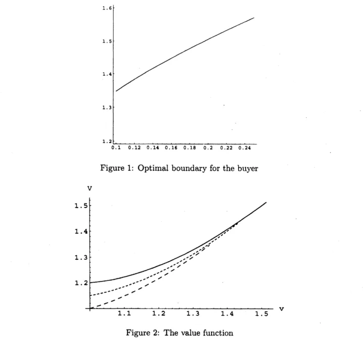
the price of callable Russian option. We set

$r=0.1,$ $d=0.09,$ $\kappa=0.3$

.

_{$p=1,$ $q=0,$ $\eta_{1}=50,$} $\lambda=3$

.

Using these parameter, $\delta^{*}$ is

0.248.

Figure 1 shows that the optimalexercise boundary

as

the penalty $\delta$ increases from

0.1

up to

$\delta^{*}$

.

From the figure,

we

can

see

that the optimal boundary $v_{0}$ is increasing in the penalty $\delta$

.

Figure 2

demonstrates

the value functionofthe callable Russianoption with jumps. Dashed

lines represent $\delta=0.1,0.15$ from thebottom. Real line _represents $\delta=0.2$

.

From this figure, we

can

recognize that $V(v)$ is

convex

and increasing _in $v$

.

References

[1] Cvitanic, J. andKaratzas, I., Backward stochastic differentialequations with reflection and

Dynkingames, The Annals

_of

Probability, 24, 2024-2056, (1996).

[2] Kifer, Y., Gameoptions, Finance and Stochastics, 4, 443-463, (2000).

[3] Kou,

S.G.

and H. Wang, First

passage

times for a jump diffusion process, Advances in

Applied Probability, 35, 504-531, (2003).

[4] Kou,

_S.G.

and H. Wang, Option Pricing Under

a

Double Exponential Jump Diffusion

Figure 1: Optimal boundary for the buyer

V

Figure 2: The value function

[5] Kyprianou, A.E.,

Some

calculations for Israeli options, Finance

and

Stochastics, 8, 73-86, (2004).

[6] Shepp, L.A. and Shiryaev, A.N., TheRussianoption: reducedregret, The

Annals

_of

Applied

Probability, 3, 631-640, (1993).

[7] Shepp, L.A. and Shiryaev, A.N., A

new

look at pricing of the ‘Russian option‘, Theory

_of

Prvbability and its Applications, 39, 103-119, (1994).

[8] Suzuki, A. and K. Sawaki, The Pricing of Callable Russian Options and Their Optimal

Boundaries, preprint.

[9] Suzuki, A. and K. Sawaki, The Valuation of Russian Options for

a

Double Exponential Jump Diffusion Process, Proceedings

_of

International Workshop on Recent Advances in