Construction of the $\Phi^4_4$ quantum field theory on noncommutative Moyal space (Applications of Renormalization Group Methods in Mathematical Sciences)

Construction

of

the

$\Phi_{4}^{4}$

quantum field

theory

on

noncommutative

Moyal

space

Harald

GROSSE1

and

Raimar

WULKENHAAR2

1 _Fakult\"at

_f\"ur

_{Physik, Universit\"at Wien}

Boltzmanngasse 5,

A-1090

Wien, Austria

2 _{Mathematisches Institut der}

Westf\"alischen

Wilhelms-Universit\"at

Einsteinstrafle

62,

_D-48149

M\"unster, Germany

Abstract

We review

our

recent construction of the $\phi^{4}$-model on four-dimensional

Moyal space.

A

milestone is the exact solution

of

the quartic matrix model $\mathcal{Z}[E, J]=\int d\Phi\exp(trace(J\Phi-E\Phi^{2}-\frac{\lambda}{4}\Phi^{4}))$ in terms of the

solu-tion ofa non-linear equationfor the 2-point function and the eigenvalues

of$E$. The$\beta$-function vanishes identically. For the Moyal model, the

the-oryof Carlemantypesingular integral equations reduces the construction to

a

fixed point problem. Its numerical solution reveals a second-order

phase transition at $\lambda_{c}\approx-0.396$ and aphasetransition ofinfinite order at

$\lambda=0$. The resulting Schwinger functions in position space

are

symmet-ric and invariant under the full Euclidean group. They

are

only sensitive to diagonal matrix correlation functions, and clustering is violated. The

Schwinger 2-point function is reflection positive iff the diagonal matrix 2-point function is a Stieltjes function. Numerically this

seems

to be the

case

for coupling constants $\lambda\in[\lambda_{c}, 0].$

1

Introduction

Perturbatively renormalised quantum field theory is an

enormous

phenomeno-logical success, a

success

which lacks a mathematical understanding. The

per-turbation series is at best an asymptotic expansion which cannot converge at physical coupling constants. Some physical effects such

as

confinement

are

out of reach for perturbation theory. In two and partly three dimensions,

meth-ods of constructive physics [GJ87, Riv91], often combined with the Euclidean

approach [Sch59, OS73, OS75], were used to rigorously establish quantum field

theory models.

In four dimensions there

was

little

success so

far. It is generally believed that due toasymptoticfreedom,

non-Abelian gauge

theory (i.e. Yang-Millstheory)

has

[email protected]

the

chance

of

a

rigorous

construction.

But this is

a

hard problem [JW00]. What

makes it

so

difficult is the fact that any simpler model such as quantum electro-dynamics

or

the $\lambda\phi^{4}$-model cannot be constructed in four dimensions (Landau

ghost problem $[LAK54a, LAK54b, LAK54c]$

or

triviality [Aiz81, Fr\"o82

One

of the main

difficulties

is the non-linearity

of

the

models

under

consider-ation.

Fixed

point methods provide

a

standard

approach to non-linear problems, but they

are

rarely used in quantum field theory. In this contribution we review

a

sequence of papers $[GW12b, GW13b, GW14]$ in which

we

successfully used

symmetry and fixed point methods to exactly solve a toy model for

a

quantum

field theory in four dimensions.

1. Following $[GW12b]$_,

we

_{show in}

sec.

_{2 that the} quartic matrix model $\mathcal{Z}=$

$\int \mathcal{D}[\Phi]\exp(tr(J\Phi-E\Phi^{2}-\frac{\lambda}{4}\Phi^{4}))$ is exactly solvable in terms of the solution

ofanon-linear equation. This

can

be tracedback to

a

Ward identity forthe

$U(\infty)$ group action. As by-product

we

find that any renormalisable quartic

matrix model has vanishing $\beta$-function. All these steps

are

completely

elementary.

2.

Self-dual

$\phi_{4}^{4}$-theory

on

Moyal space $[GW05b, GW05c]$ is of that type. For

extreme noncommutativity $\thetaarrow\infty$, and after careful discussion of

ther-modynamic and continuum limit, the non-linear equation is reduced to

a fixed-point problem $[GW12b]$ which has a unique non-perturbative and

non-trivial solution for $\lambda<0$ [GW14].

Sec.

3 reviews this work. The key

step is the observation that

a

certain difference function satisfies

a

linear

singular integralequationofCarlemantype [Car22, $Ri57$_{]. We also} present

some

numerical results, contained in work in progress [GW14], which show

evidence for phase transitions.

3. Following $[GW13b]$,

we

identify in

sec.

4

a

limit to Schwinger functions for

a

scalar field

on

$\mathbb{R}^{4}$

. Surprisingly for

a

highly noncommutative model, these Schwinger

functions

show full Euclidean symmetry. Otherwise they have unusual properties such

as

absent momentum transfer in interaction

processes. This

seems

to suggest triviality, but the numerical investigation [GW14] of the 2-point function shows scattering remnants from a

non-commutative geometrical substructure. Most surprisingly, the Schwinger

2-point function seems to be reflection positive in one of its phases.

2

Exact

solution of the

quartic matrix

model

For

us a

‘matrix’ is

a

compact (Hilbert-Schmidt) operator on Hilbert space $H=$

$L^{2}(I, \mu)$. Such operators $\Phi\in \mathcal{L}^{2}(H)$

can

be represented by integral kernel

oper-ators $( \Phi v)_{a}=\int_{I}d\mu_{b}\Phi_{ab}v_{b}$

.

Then all natural matrix operations such

as

product,

adjoint and trace have counterparts $( \Phi\Phi’)_{ab}=\int_{I}d\mu_{c}\Phi_{ac}\Phi_{cb}’,$ $(\Phi^{*})_{ab}=\overline{\Phi_{ba}}$ and $tr(\Phi\Phi’)=\int_{I}d\mu_{a}(\Phi\Phi’)_{aa}$ in $\mathcal{L}^{2}(H)$.

To define a Euclidean quantum

_field

theory for a matrix $\Phi\in \mathcal{L}^{2}(H)$ we give

ourselves an action functional

$S[\Phi]=Vtr(E\Phi^{2}+P[\Phi])$ _{. (1)}

Here, $P[\Phi]$ is a polynomial in $\Phi$ with scalar coefficients, and this alone would

be

a

familiar action in the theory of matrix models [DGZ95]. To be closer to

field theory on $a$ (compact) manifold $\mathcal{M}$

we

add the analogue of the kinetic term $\int_{\mathcal{M}}dx(-\triangle\phi)\phi$, that is,

we

require the external matrix $E$ to be an unbounded selfadjoint positive operator

on

$H$ with compact resolvent. The volume $V$ will

play

a

crucial r\^ole. The construction involves several regularisation and limiting

procedures. One such regularisation consists in a finite size $\mathcal{N}$ for the matrices,

and $V$ will be a certain function of$\mathcal{N}$which together with$\mathcal{N}$ is sent to

$\infty.$

Adding

a source

term to the action,

we

define the partition junction

as

$\mathcal{Z}[J]=\int \mathcal{D}[\Phi]\exp(-S[\Phi]+Vtr(\Phi J))$ , (2) where $\mathcal{D}[\Phi]$ is the extension of the Lebesgue

measure

from finite-rank operators

to $\mathcal{L}^{2}(H)$ and $J$

a

test function matrix. For absent $P[\Phi]\mapsto 0$ in (1), $\frac{\mathcal{D}[\Phi]}{\mathcal{Z}[0]}$ would

be the $Gaui3ian$ _{measure of covariance determined by} $E$. What we want, and

whatweachieve, $istoc$onstruct $\frac{\mathcal{D}[\Phi]}{z\}^{0]}}forP[\Phi]=\frac{\lambda}{4,S}\Phi^{4}inthel$imit V

$arrow\infty.$

Sucha

limit cannot b$ee$xpected f$or\mathcal{Z}.$ nstead,

$wepastotheg$

enerating functional

$\log \mathcal{Z}[J]$ of connected correlation functions,

$\langle\varphi_{a_{1}b_{1}}\ldots\varphi_{ab_{N}}N\rangle_{c}=\frac{\partial^{N}1og.\mathcal{Z}[J]}{\partial J_{b_{1}a_{1}}..\partial J_{b_{N}a_{N}}}|_{J=0}$ (3)

2.1 Ward identity and topological expansion

Unitaryoperators $U$belongingto

an

appropriate unitisation of thecompact

oper-ators on$H$ give rise to a transformation $\Phi\mapsto\tilde{\Phi}=U\Phi U^{*}$_{. Since $UU^{*}=U^{*}U=id$}

and because the space of selfadjoint compact operators is invariant under the ad-joint action, we have

$\int \mathcal{D}[\Phi]\exp(-S[\Phi]+Vtr(\Phi J))=\int \mathcal{D}[\tilde{\Phi}]\exp(-S[\tilde{\Phi}]+Vtr(\tilde{\Phi}J))$ . Unitary invariance $\mathcal{D}[\tilde{\Phi}]=\mathcal{D}[\Phi]$ ofthe Lebesgue

measure

implies

$0= \int \mathcal{D}[\Phi\{\exp(-S[\Phi]+Vtr(\Phi J))-\exp(-S[\tilde{\Phi}]+Vtr(\tilde{\Phi}J))\}$

Note that the integrand $\{$. . . $\}$ itself does not vanish because $tr(E\Phi^{2})$ and $tr(\Phi J)$

are

not unitarily invariant. Linearisation of $U$ about the identity operator leads

to the Ward identity

We

can

always place ourselves in

an

orthonormal basis of $H$ where $E$ is diagonal

(but $J$ is not). Since $E$ is of compact resolvent, $E$ has eigenvalues _{$E_{a}>0$} of finite multiplicity $\mu_{a}$. We thus label the matrices by

an

enumeration of the

(necessarily discrete) eigenvalues of $E$ and

an

enumeration

of

the

basis

vectors

of

the

finite-dimensional

eigenspaces. Writing $\Phi$ in

$\{$. . . $\}$

of

(4)

as

functional

derivative $\Phi_{ab}=\frac{\partial}{V\partial J_{ba}}$,

we

have proved (first obtained in [DGMR07]):

Proposition 1 The partition

_function

$Z[J]$

of

the matrix model

defined

by the

external matrix $E$

satisfies

the $|I|\cross|I|$ Ward identities

$0= \sum_{n\in I}(\frac{(E_{a}-E_{p})}{V}\frac{\partial^{2}\mathcal{Z}}{\partialJ_{an}\partial J_{np}}+J_{pn}\frac{\partial \mathcal{Z}}{\partial J_{an}}-J_{na}\frac{\partial \mathcal{Z}}{\partial J_{np}})$ (5)

Without loss of generality

we can

assume

that the map $I\ni m\mapsto E_{m}\in \mathbb{R}_{+}$ is

injective. Namely, correlation functionswill only depend

on

the set ofeigenvalues

$(E_{m})$

of

$E$. Partitioning the index set $I$ into equivalence classes _$[m]$ which have

the

same

$E_{m}$, the index

sum

over

a

function

that only depends

on

$E_{m}$ becomes $\sum_{m\in I}f(m)=\sum_{[m]\in[I]}\mu_{[m]}f([m])$. Therefore, at the price of adding

a

measure

$\mu_{[m]}=\dim ker(E-E_{m}id)$,

we can

assume

that $m\mapsto E_{m}$ is injective.

In

a

perturbative expansion, Feynman graphs in matrix models

are

ribbon

graphs. Viewed

as

simplicial complexes, they encode the topology $(B, g)$ of

a

genus-g

Riemann surface with $B$ boundary components (or punctures, marked

points, holes, faces).

Some

simple examples for $P[\Phi]=\Phi^{4}$

are:

$A$

$d_{d}$

Since$E$ is diagonal, the matrixindex isconserved alongeach strandoftheribbon

graph. We have to distinguish between internal faces (with constant matrix

index) and broken faces which constitute the boundary components. Such

a

boundary face is characterised by $N_{k}\geq 1$ external double lines to which we

attach the

source

matrix $J$. Conservation ofthe matrix index along each strand

implies that the right index of $J_{ab}$ coincides with the left index of another $J_{bc},$

or of the

same

$J_{bb}$. Accordingly, the $k^{th}$ boundary component carries

a

cycle

$J_{p_{1}\ldots p_{N_{k}}}^{N_{k}}$ $:= \prod_{j=1}^{N_{k}}J_{p_{j}p_{j+1}}$ of $N_{k}$ external sources, with $N_{k}+1\equiv 1.$

Being interested in

a

non-perturbative solution,

we

will not expand the par-tition

function

into ribbon graphs. But

we

keep the topological information and

expand $\log \mathcal{Z}[J]$ according to the cycle structure:

$\log\frac{\mathcal{Z}[J]}{\mathcal{Z}[0]}=\sum_{B=1}^{\infty}\sum_{1\leq N_{1}\leq\cdots\leq N_{B}}^{\infty}\sum_{p_{1)}^{\beta}\ldots,p_{N_{\beta}}^{\beta}\in I}\frac{V^{2.-B}}{S_{N_{1}..N_{B}}}G_{|p_{1}^{1}\ldots p_{N_{1}}^{1}|\ldots|p_{1}^{B}\ldots p_{N_{B}}^{B}|}\prod_{\beta=1}^{B}(\frac{J^{N_{\beta}}p_{1}^{\beta}\ldots p_{N_{\beta}}^{\beta}}{N_{\beta}})$

(6)

The symmetry factor $S_{N_{1}\ldots N_{B}}$ is obtained

as

follows: If $\nu_{i}$ of the $B$ numbers $N_{\beta}$

in

a

given tuple $(N_{1}, \ldots, N_{B})$

are

equal to $i$, then $S_{N_{1}\ldots N_{B}}= \prod_{i=1}^{N_{B}}\nu_{i}!.$

Next

we

turn the Ward identity (5) for injective $m\mapsto E_{m}$ into a formula for the second derivative $\sum_{n\in I\partial J_{an}\partial J_{np}}^{\partial^{2}Z[J]}$ of the partition function. The $J$-cycle

structure in $\log \mathcal{Z}$ creates

$\bullet$ singular contributions $\sim\delta_{ap},$

$\bullet$ regular contributions present for all

$a,p$:

Theorem 2

$\sum\frac{\partial^{2}\mathcal{Z}[J]}{\partial J_{an}\partial J_{np}}=\delta_{ap}\{V^{2}\sum\frac{J_{P_{1}}\cdots J_{P_{K}}}{S_{(K)}}(\sum\frac{G_{|an|P_{1}|\ldots|P_{K}|}}{V^{|K|+1}}+\frac{G_{|a|a|P_{1}|\ldots|P_{K}|}}{V^{|K|+2}}$

$n\in I$ _(K) $n\in I$

$+ \sum \sum \frac{G_{|q_{1}aq_{1}\ldots q_{r}|P_{1}|\ldots|P_{K}|^{J_{q_{1}\ldots q_{r}}^{r}}}}{V^{|K|+1}})$

$r\geq 1q_{1},\ldots\rangle q_{r}\in I$

$+V^{4} \sum\frac{J_{P_{1}}\cdots J_{P_{K}}J_{Q_{1}}\cdots J_{Q_{K’}}}{S_{(K)}S_{(K’)}}\frac{G_{|a|P_{1}|\ldots|P_{K}|}}{V|K|+1}\frac{G_{|a|Q_{1}|\ldots|Q_{K’}|}}{V|K|+1}\}\mathcal{Z}[J]$

$(K),(K’)$

$+ \frac{V}{E_{p}-E_{a}}\sum(J_{pn}\frac{\partial \mathcal{Z}[I]}{\partial J_{an}}-J_{na}\frac{\partial \mathcal{Z}[I]}{\partial I_{np}})$ (7)

$n\in I$

Proof.

We identify the following four

sources

of

a

singular contribution $\sim\delta_{ap}$:

1. $\sum_{n}\frac{\partial^{2}}{\partial J_{an}\partial J_{np}}\sum_{q_{1},q_{2_{\rangle}}}..,$

$G \ldots|q_{1}q_{2}|\ldots(\frac{J_{q_{1}q_{2}}J_{q_{2}q_{1}}^{\downarrow}\downarrow}{2})\prod J$

2. $\sum_{n}\frac{\partial^{2}}{\partial J_{an}\partial J_{np}}\sum_{q_{1},q_{2},\rangle}..G\ldots|q_{1}|\ldots|q_{2}|\ldots(\frac{J_{q_{1}q_{1}}^{\downarrow}}{1})(\frac{J_{q_{2}q_{2}}^{\downarrow}}{1})\prod J$

$\downarrow$

3.

$\sum_{n}\frac{\partial}{\partial J_{an}}\frac{\partial}{\partial J_{np}}\ldots\sum_{q_{0,)}q_{r+1}}G.\cdot,\cdot|q0q_{1}\ldots q_{r}q_{r+1}|\ldots(\frac{J_{q0q_{1}}J_{q_{1}q_{2}}\cdots J_{q_{r}q_{r+1}}J_{q_{r+1}q0}}{r+2})\prod J$

4. $\sum_{n}\frac{\partial^{2}}{\partial J_{an}\partial\sqrt{}np}[\sum_{q_{1}},$

$G \ldots|q_{1}|\ldots(\frac{J_{q_{1}q_{1}}^{\downarrow}}{1})\prod J][\sum_{q_{2}}G\ldots|q_{2}|\ldots(\frac{J_{q_{2}q_{2}}^{\downarrow}}{1})\prod J]$

All

other types

of

derivatives,

collected

into $( \sum_{n\in I\partial J_{an}\partial J_{np}}^{\partial^{2}Z[J]})_{reg}$, persist

for

_{$a\neq p.$}

For $p\neq a$

we

clearly have

$( \sum_{n\in I}\frac{\partial^{2}\mathcal{Z}[J]}{\partial J_{an}\partial J_{np}})_{reg}=\sum_{n\in I}\frac{\partial^{2}\mathcal{Z}[J]}{\partial J_{an}\partial J_{np}}|_{a\neq p}=\frac{V}{E_{p}-E_{a}}(J_{pn}\frac{\partial \mathcal{Z}}{\partial J_{an}}-J_{na}\frac{\partial \mathcal{Z}}{\partial J_{np}})$ , (8)

where the last equality isthe Ward identity (5), divided by $\frac{E_{p}-E_{a}}{V}\neq 0$. By

a

con-tinuity argument, the rightmost term in (8) must agree with $( \sum_{n\in I\partial J_{an}\partial J_{np}}^{\partial^{2}Z[J]})_{reg}$

also in the limit $parrow a$, and this finishes the proof. $\square$

2.2

Schwinger-Dyson equations

We

can

write the action

as

$S= \frac{V}{2}\sum_{a,b}(E_{a}+E_{b})\Phi_{ab}\Phi_{ba}+VS_{int}[\Phi]$, where $E_{a}$

are

the eigenvalues of$E$. Functional integration yields, up to

an

irrelevant constant,

$\mathcal{Z}[J]=e^{-VS_{int[\frac{\partial}{V\^{o} J}]}}e^{\frac{V}{2}\langle J,J\rangle_{E}}, \langle J, J\rangle_{E}:=\sum_{m,n\in I}\frac{\sqrt{}J}{E_{m}+E_{n}}$ (9)

Instead of

a

perturbative expansion of $e^{-VS_{int}[\frac{\^{o}}{V\partial J}]}$

,

we

apply such $J$-derivatives

to (9) that they give rise to

a

correlation function $G$

on

the lhs.

On

the rhs of

(9), these external derivatives combine with internal derivatives from $S_{int}[ \frac{\partial}{V\partial J}]$

to certain identities for $G$ These Schwinger-Dyson equations are often of little

use

because they express

an

$N$-point function in terms of_$(N+2)$-point functions. In the

field-theoretical

matrix models under consideration, the Ward identity

(7) lets this tower of Schwinger-Dyson equation collapse. To

see

this

we

consider the2-point function$G_{|ab|}$ for$a\neq b$. Accordingto (6), $G_{|ab|}$ isobtainedby deriving

(9) with respect to $J_{ba}$ and $J_{ab}$:

$G_{|ab|}= \frac{1}{V\mathcal{Z}[0]}\frac{\partial^{2}\mathcal{Z}[I]}{\partial I_{ba}\partial I_{ab}}|_{J=0}$

$notc$ontribute f

$ora\neq b)($

disconnected p$artofZ$ does

$= \frac{1}{V\mathcal{Z}[0]}\{\frac{\partial}{\partial I_{ba}}e^{-VS_{int}[\frac{\partial}{V\partial J}]}\frac{\partial}{\partial J_{ab}}e^{\frac{V}{2}\langle J,J\rangle_{E}}\}_{J=0}$

$= \frac{1}{(E_{a}+E_{b})\mathcal{Z}[0]}\{\frac{\partial}{\partial J_{ba}}e^{-VS_{i\mathfrak{n}t}[\frac{\partial}{V\partial J}]}I_{ba}e^{\frac{V}{2}\langle J,J\rangle_{E}}\}_{J=0}$

$= \frac{1}{E_{a}+E_{b}}+\frac{1}{(E_{a}+E_{b})\mathcal{Z}[0]}\{(\Phi_{ab}\frac{\partial(-VS_{int})}{\partial\Phi_{ab}})[\frac{\partial}{V\partial I}]\}\mathcal{Z}[J]|_{J=0}$ (10)

which w

$eknowfrom.Incaseoftheq$

uartic matrix m

$ode1P[\Phi]=Nowo$

bserve t

have $\frac{\partial(-VS_{int})}{\partial\Phi_{ab}}=-\lambda V\sum_{n,p\in I}\Phi_{bp}\Phi_{pn}\Phi_{na}$, hence

$( \Phi_{ab}\frac{\partial(-VS_{int})}{\partial\Phi_{ab}})[\frac{\partial}{V\partial J}]=-\frac{\lambda}{V^{3}}\sum_{p,n\in I}\frac{\partial^{2}}{\partialJ_{pb}\partial J_{ba}}\frac{\partial^{2}}{\partial J_{an}\partial J_{np}},$

and the Schwinger-Dyson equation (10) for $G_{|ab|}$ becomes with (7)

$G_{|ab|}= \frac{1}{E_{a}+E_{b}}-\frac{\lambda}{V^{3}(E_{a}+E_{b})\mathcal{Z}[0]}\sum_{p\in I}\frac{\partial^{2}}{\partial J_{pb}\partial J_{ba}}\sum_{n\in I}\frac{\partial^{2}\mathcal{Z}}{\partial J_{an}\partial J_{np}}|_{J=0}$

$= \frac{1}{E_{a}+E_{b}}-\frac{\lambda}{V(E_{a}+E_{b})\mathcal{Z}[0]}\frac{\partial^{2}}{\partial J_{ab}\partial J_{ba}}\{$

$( \sum_{n\in I}\frac{G_{|an|}}{V}+\sum_{n,q,r\in I}\frac{G_{|an|qr|}}{V^{2}}\frac{J_{qr}J_{rq}}{2}+\sum_{n,q,r\in I}\frac{G_{|an|q|r|}}{V^{3}}\frac{J_{qq}}{1}\frac{J_{rr}}{1}$

$+ \frac{G_{|a|a|}}{V^{2}}+\sum_{q,r\in I}\frac{G_{|a|a|qr|}}{V^{3}}\frac{J_{qr}J_{rq}}{2}+\sum_{q,r\in I}\frac{G_{|a|a|q|r|}}{V^{4}}\frac{J_{qq}}{1}\frac{J_{rr}}{1}$

$+ \sum_{q,r\in I}\frac{G_{|qaqr|}}{V}J_{qr}J_{rq}+V^{2}\frac{G_{|a|q|}}{V^{2}}\frac{J_{qq}}{1}\frac{G_{|a|r|}}{V^{2}}\frac{J_{rr}}{1})\mathcal{Z}[J]\}J=0$

$- \frac{\lambda}{V^{2}(E_{a}+E_{b})\mathcal{Z}[0]}\sum_{p\in I}\frac{(\frac{\partial^{2}\mathcal{Z}\lceil J]}{\partial J_{ab}\partial J_{ba}}+\frac{\partial^{2}\mathcal{Z}[J]}{\partial J_{aa}\partial J_{bb}}-\frac{\partial^{2}\mathcal{Z}[J]}{\partial J_{pb}\partial J_{bp}})}{E_{p}-E_{a}}J=0$

(11)

Taking $\frac{\partial^{2}Z[J]}{\partial J_{pb}\partial J_{bp}}=(VG_{|pb|}+\delta_{pb}G_{|p|b|})\mathcal{Z}[0]+\mathcal{O}(J)$ and $\frac{\partial J}{\partial J_{ab}}=0$ for $a\neq b$ into

account,

we

have proved:

Proposition 3 The 2-point

_function

_of

a quartic matrix model with action $S=$

$V tr(E\Phi^{2}+\frac{\lambda}{4}\Phi^{4})$

satisfies for

injective $m\mapsto E_{m}$ the Schwinger-Dyson equation

$G_{|ab|}= \frac{1}{E_{a}+E_{b}}-\frac{\lambda}{E_{a}+E_{b}}\frac{1}{V}\sum_{p\in I}(G_{|ab|}G_{|ap|}-\frac{G_{|pb|}-G_{|ab|}}{E_{p}-E_{a}})$ $\}$ (12a)

$- \frac{\lambda}{V^{2}(E_{a}+E_{b})}(G_{|a|a|}G_{|ab|}+\frac{1}{V}\sum_{n\in I}G_{|an|ab|}$

(12b)

$+G_{|aaab|}+G_{|baba|}- \frac{G_{|b|b|}-G_{|a|b|}}{E_{b}-E_{a}})$

$- \frac{\lambda}{V^{4}(E_{a}+E_{b})}G_{|a|a|ab|} \}$ (12c)

It

can

be checked that in a genus expansion $G$ $= \sum_{g=0}^{\infty}V^{-2g}G^{(g)}$ (which is

probably not convergent but Borel summable), precisely the line (12a) preserves

Moreover, in a scaling limit $Varrow\infty$ with $\frac{1}{V}\sum_{p\in I}$ finite, the exact

Schwinger-Dyson equationfor $G_{|ab|}$ coincides with its restriction (12a) to planar sector$g=0,$

a

closed non-linear equation for $G_{|ab|}^{(0)}$ alone:

$G_{|ab|}^{(0)}= \frac{1}{E_{a}+E_{b}}-\frac{\lambda}{E_{a}+E_{b}}\frac{1}{V}\sum_{p\in I}(G_{|ab|}^{(0)}G_{|ap|}^{(0)}-\frac{G_{|pb|}^{(0)}-G_{|ab|}^{(0)}}{E_{p}-E_{a}})$ (13)

Wehave derived in 2007/08this self-consistency equation for the Moyal model by

the graphical method proposed by [DGMR07]. In this form, (13) is meaningless

because $\sum_{p\in I}$ diverges. In

2009 we

solved the renormalisation problem, namely

the renormalisation of infinitely many Feynman graphs at

once

[GW09]. This renormalisation increases the non-linearity. In [GW09]

we

have solved (13)

per-turbatively to $\mathcal{O}(\lambda^{3})$. After several years of setbacks with the non-perturbative

solution,

a

breakthrough

came

in

2012:

The equation (13)

can

be turned into

an

equation which is linear in the difference $G_{|ab|}^{(0)}-G_{|a0|}^{(0)}$ to the boundary and

non-linear only in $G_{|a0|}^{(0)}!$

A similar calculation gives the Schwinger-Dyson equation for higher $N$-point functions:

$G_{|ab_{1}\ldots b_{N-1}|}$

$=- \frac{\lambda}{E_{a}+E_{b_{1}}}(\frac{1}{V}\sum_{p\in I}(G_{|ap|}G_{|ab_{1}\ldots b_{N-1}|}-\frac{G_{|pb_{1}\ldots b_{N-1}|}-G_{|ab_{1}\ldots b_{N-1}|}}{E_{p}-E_{a}})$

$-G_{|b_{1}\ldots b_{2l}|} \frac{G_{|b_{2l+1}\ldots b_{N-1}a|}-G_{|b_{2l+1}\ldots b_{N-1}b_{2l}|}}{E_{b_{2l}}-E_{a}})\frac{N-2}{\sum 2}l=1$

(14a)

$- \frac{\lambda}{V^{2}(E_{a}+E_{b_{1}})}(G_{|a|a|}G_{|ab_{1}\ldots b_{N-1}|}+\sum_{k=1}^{N-1}G_{|b_{1}\ldots b_{k}ab_{k}\ldots b_{N-1}a|}$

$+G_{|aaab_{1}\ldots b_{N-1}|}+ \frac{1}{V}\sum_{n\in I}G_{|an|ab_{1}\ldots b_{N-1}|}$ (14b)

$- \sum_{k=1}^{N-1}\frac{G_{|b_{1}\ldots b_{k}|b_{k+1}\ldots b_{N-1}b_{k}|}-G_{|b_{1}\ldots b_{k}|b_{k+1}\ldots b_{N-1}a|}}{E_{b_{k}}-E_{a}})$

$- \frac{\lambda}{V^{4}(E_{a}+E_{b_{1}})}G_{|a|a|ab_{1}\ldots b_{N-1}|}$ $\}$ (14c) Again, the first lines (14a) preserve the genus, whereas $g\mapsto g+1$ in (14b) and $g\mapsto g+2$ in (14c). The planar sector $G_{|ab_{1}\ldots b_{N-1}|}^{(0)}$, exact for $Varrow\infty$ with $\frac{1}{V}\sum_{p\in I}$

finite, is a linear inhomogeneous equation with inductively known parameters. It turns out that a real theory with $\Phi=\Phi^{*}$ admits

a

short-cut which directly

gives the higher $N$-point functions without any index summation. Since the

equations for $G$

are

real and $\overline{J_{ab}}=J_{ba}$, the reality $\mathcal{Z}=\overline{\mathcal{Z}}$

under orientation reversal

$G_{|p_{0}^{1}p_{1}^{1}\ldots p_{N_{1}-1}^{1}|\ldots|p_{0}^{B}p_{1}^{B}\ldots p_{N_{B}-1}^{B}|}=G_{|p_{0}^{1}p_{N_{1}-1}^{1}\ldots p_{1}^{1}|\ldots|p_{0}^{B}p_{N_{B}-1}^{B}\ldots p_{1}^{B}|}$ (15) Whereas empty for $G_{|ab|}$, in $(E_{a}+E_{b_{1}})G_{ab_{1}b_{2}\ldots b_{N-1}}-(E_{a}+E_{b_{N-1}})G_{ab_{N-1}\ldots b_{2}b_{1}}$ the

identities (15) lead to many cancellations which result in a universal algebraic recursion formula:

Proposition 4

$G_{|b_{0}b_{1}\ldots b_{N-1}|}=(- \lambda)^{\frac{N-2}{\sum_{l=1}^{2}}}\frac{G_{|b_{0}b_{1}\ldots b_{2l-1}|G_{|b_{2l}b_{2l+1}\ldots b_{N-1}|}-G_{|b_{2l}b_{1}\ldots b_{2l-1}|}G_{|b_{0}b_{2l+1}\ldots b_{N-1}|}}}{(E_{b_{0}}-E_{b_{2\mathfrak{l}}})(E_{b_{1}}-E_{b_{N-1}})}$

$+ \frac{(-\lambda)}{V^{2}}\sum_{k=1}^{N-1}\frac{G_{|b_{0}b_{1}\ldots b_{k-1}|b_{k}b_{k+1}\ldots b_{N-1}|}-G_{|b_{k}b_{1}\ldots b_{k-1}|b_{0}b_{k+1}\ldots b_{N-1}|}}{(E_{b_{0}}-E_{b_{k}})(E_{b_{1}}-E_{b_{N-1}})}$ (16)

The last line of (16) increases the genus and is absent in $G^{(0)}$

$|b_{0}b_{1}\ldots b_{N-1}|$. Instead of

giving the general proof, let

us

look at the

case

$N=4$. Then (14), multiplied by

$E_{a}-E_{b_{1}}$, reads $(E_{a}-E_{b})G_{|abcd|}$ $=(- \lambda)(\frac{1}{V}\sum_{p\in I}(G_{|ap|}G_{|abcd|}-\frac{G_{|pbcd|}-G_{|abcd|}}{E_{p}-E_{a}})-G_{|bc|}\frac{G_{|da|}-G_{|dc|}}{E_{c}-E_{a}})$ $- \frac{\lambda}{V^{2}}(G_{|a|a|}G_{|abcd|}+G_{|babcda|}+G_{|bcacda|}+G_{|bcdada|}+G_{|aaabcd|}+\frac{1}{V}\sum_{p\in I}G_{|ap|abcd|}$ $- \frac{G_{|b|cdb|}-G_{|b|cda|}}{E_{b}-E_{a}}-\frac{G_{|bc|dc|}-G_{|bc|da|}}{E_{c}-E_{a}}-\frac{G_{|bcd|d|}-G_{|bcd|a|}}{E_{d}-E_{a}})$ $- \frac{\lambda}{V^{4}}G_{|a|a|abcd|}$ (17)

Write down the

same

equation but with $brightarrow d$, and take the difference between

these equations. Then most terms cancel because by (15)

we

have the

equal-ities $G_{|abcd|}=G_{|adcb|},$ $G_{|pbcd|}=G_{|pdcb|)}G_{|babcda|}=G_{|dcbaba|},$ $G_{|bcacda|}=G_{|dcacba|},$ $G_{|bcdada|}=G_{|dadcba|},$ $G_{|aaabcd|}=G_{|aaadcb|},$ $G_{|ap|abcd|}=G_{|ap|adcb|},$ $G_{|b|cdb|}=G_{|dcb|b|},$ $G_{|bc|dc|}=G_{|dc|bc|},$ $G_{|bcd|d|}=G_{|d|cbd|}$ and $G_{|a|a|abcd|}=G_{|a|a|adcb|}$. Altogether, the

difference (17)$-(17)_{brightarrow d}$ reads after cancellation

$(E_{d}-E_{b})G_{|abcd|}=(- \lambda)\frac{G_{|ab|}G_{|cd|}-G_{|ad|}G_{|cb|}}{E_{c}-E_{a}}$

$- \frac{\lambda}{V^{2}}(\frac{G_{|b|cda|}-G_{|a|cdb|}}{E_{b}-E_{a}}+\frac{G_{|bc|da|}-G_{|ba|dc|}}{E_{c}-E_{a}}+\frac{G_{|a|bcd|}-G_{|d|bca|}}{E_{d}-E_{a}})$ ,

For completeness, we list in the appendix the Schwinger-Dyson equation for

$B=2$ boundary components.

Wemake the following keyobservation: An affine transformation$E\mapsto ZE+C$

together with

an

adjusted rescaling $\lambda\mapsto Z^{2}\lambda$

leaves

the

algebraic equations (16)

as

well

as

(65)

and

(66) invariant:

Theorem 5 Given a real quartic matrix model with $S=V tr(E\Phi^{2}+\frac{\lambda}{4}\Phi^{4})$ and $m\mapsto E_{m}$ injective, which determines the set$G_{|p_{1}^{1}\ldots p_{N_{1}}^{1}|\ldots|p_{1}^{B}\ldots p_{N_{B}}^{B}|}$

of

$(N_{1}+\ldots+N_{B})-$

point

_functions.

Assume that the basic

_functions

with all$N_{i}\leq 2$ are turned

finite

by $E_{a} \mapsto Z(E_{a}+\frac{\mu^{2}}{2}-\Delta\mu^{2}2aoe)$ and $\lambda\mapsto Z^{2}\lambda$. Then all

functions

with

one

$N_{i}\geq 3$

1.

are

_finite

without

_further

need

_of

a

renormalisation

_of

$\lambda,$ $i.e$. all $renor^{arrow}mal-$

isable quartic matrix models have vanishing$\beta$-function,

2. are given by universal algebraic recursion

_formulae

in terms

_of

renor,nalised

basic

_functions

with $N_{i}\leq 2.$ $\square$

Thetheorem tells

us

that vanishing of the$\beta$

-function

for the

self-dual

$\Phi_{4}^{4}$

-model

on

Moyal space (proved in [DGMR07] to all ordersin perturbation theory) is generic to all quartic matrix models, and the result

even

holds non-perturbatively!

The universal recursion formula (16) computes the planar $N$-point function

$G_{|b_{0}\ldots b_{N-1}|}$ at $B=1$

as

a sum of fractions with products of 2-point functions in

the numerator and products of differences of eigenvalues of $E$ in the

denomin-ator. This structure admits

an

interesting graphical interpretation. We draw the indices $b_{0}$, . . ._{$b_{N-1}$} in cyclic order

on

the circle $S^{1}$ and represent

a

factor $G_{b_{i}b_{j}}$

as

a

chord connecting $b_{i}$ with $b_{j}$ and a factor $\frac{1}{E_{b_{i}}-E_{b_{\grave{J}}}}$

as

an arrow from

The chords form the non-crossing chord diagrams counted by the Catalan

num-ber $C_{\frac{N}{2}}= \frac{N!}{(\frac{N}{2}+1)!\frac{N}{2}!}$. The

arrows

form two disjoint trees,

one

connecting the

even

vertices

ans one

connecting the odd vertices. By rational fraction expansion it is possible to achieve that each tree intersects the chord only in the vertices.

The assignment of trees to a given chord diagram is, in general, not unique. $A$

canonical choice is not known to

us.

2.3

Digression: Quantum gravity in two dimensions

Two-dimensional quantum gravity (see [DGZ95, ADJ97] for reviews)

can

be in-terpreted

as

theenumeration of random triangulationsof surfaces. Its asymptotic

behaviour is captured by the matrix model partition function

$\mathcal{Z}=\int \mathcal{D}[\Phi]\exp(-\mathcal{N}\sum_{n}t_{n}tr(\Phi^{n}))$ , (19)

where the integral is

over

$(\mathcal{N}\cross \mathcal{N})$-Hermitean matrices $\Phi$ and the

$t_{n}$

are

scalar

coefficients. In the limit $\mathcal{N}arrow\infty$, this series in _{$(t_{n})$} is evaluated in terms of

the $\tau$-function for the Korteweg-de Vries $(KdV)$ hierarchy. There is another

approach to topological gravity in which the partition function is

a

series in

$(t_{n})$ with coefficients given by intersection numbers of complex curves. Witten

conjectured [Wit91] that the partition functions ofthe two approaches coincide.

Thisconjecturewas proved byKontsevich [Kon82] who achieved the computation

of the intersection numbers in terms of weighted

sums

over

ribbon graphs (fat

Feynman graphs), which he proved tobegeneratedfrom the Airy function matrix

model (Kontsevich model)

$\mathcal{Z}[E]=\frac{\int \mathcal{D}[\Phi]\exp(-\frac{1}{2}tr(E\Phi^{2})+\frac{i}{6}tr(\Phi^{3}))}{\int \mathcal{D}[\Phi]\exp(-\frac{1}{2}tr(E\Phi^{2}))}$ , (20)

where $E=E^{*}>0$ _{is related to the series} $(t_{n})$ by _{$t_{n}=(2n-1)!!tr(E^{-(2n-1)})$}. The

limit $\mathcal{N}arrow\infty$ of

$\mathcal{Z}[E]$ gives the $KdV$ evolution equation, thus proving Witten’s

conjecture.

We have proved that also the quartic matrix model

is in the $large-\mathcal{N}$ limit exactly solvable in terms of the solution of

a

non-linear

equation (13). Any triangulation

can

be subdivided into

a

quadrangulation

(and vice versa). From Witten’s uniqueness argument [Wit91], $2D$ quantum gravityshould have equivalent descriptions

as

cubic (20) and quartic (21) matrix model. Understanding the precise relation between (20) and (21) would be of high interest:

1. In contrast to (21), the cubic action (20) lacks manifest positivity due to

its purely imaginary coupling constant.

2. A quartic actionadmits

a

Hubbard-Stratonovich transform whichisthe key ingredient of

a

new

approach to constructive quantumfield theory $[Riv07b]$ that avoids the cluster expansion.

3.

Conversely, the integrability

of

(20) might provide valuable information about the solution of the self-consistency equation (13).

Coloured tensor models (see [GP12, Riv13] for recent reviews) extend these

methods to quantum gravity in $D\geq 3$. They became

a

very active domain of

research after understanding [GurlO] of the analogue of the $large-\mathcal{N}$ behaviour of

matrix models $[tHo74]$_{. They have} Schwinger-Dyson equations (see

e.g.

[Bon12])

and action of the $U(\infty)$ group. It might be promising to extend

our

techniques

to coloured tensor models.

3

$\Phi_{4}^{4}$

-theory

on

Moyal space

as a

fixed point problem

3.1

Preliminaries

Taking the renormalisation group [WK74] serious,

we

would expect that

Gen-eral Relativity, because not renormalisable, is marginal and hence scaled away. Presence of gravity tells

us

that the scaling must stop at

some

length scale, and from the weakness of the gravitational coupling constant

one

deduces the value of that scale: the Planck length $10^{-35}m$_{. There, the geometry of nature is}

ex-pected to differ from the familiar structure of

a

differentiable manifold.

One

of

many candidates for Planck scale physics is noncommutative geometry [Con94],

a

vast reformulation of geometry and topology in the language of operator

al-gebras. The focus is shifted from manifolds to generalisations of the algebra of functions. This concept proved very successful in understanding the geometry of

the

Standard Model

of particle physics

as

Riemannian

geometry of

a

space which

is the product of

a

manifold with

a

discrete space [Con96, CC96].

A

large class of examples of noncommutative geometries

comes

from

deform-ations ofthe algebra offunctions

on

manifolds. Schwartz functions

on

Euclidean

space $\mathbb{R}^{4}$

this group action induces a noncommutative associative product on the space of Schwartz functions, the Moyal product:

$(f \star g)(x)=\int_{\mathbb{R}^{4}\cross \mathbb{R}^{4}}\frac{dydk}{(2\pi)^{4}}f(x+\frac{1}{2}\Theta k)g(x+y)e^{i\langle k,y\rangle},$ $\Theta=-\Theta^{t}\in M_{4}(\mathbb{R})$ . (22)

Whether

or

not the Moyal space $(\mathbb{R}^{4}, \star)$ is relevant for Planck scale physics

is pure speculation (although a refinement can be justified by uncertainty rela-tions for position operators [DFR95]). In any

case

the Moyal space is

a

nice toy model

on

which it is easy to formulate and to study (quantum) field theories. To formulate a Euclidean quantum field theory on Moyal space it is, at first sight, enough to replace in the action of a usual field theory the pointwise product of functions by the $\star$-product. The simplest example is the $\phi_{4}^{4}$-model with action

$S[ \phi]=\int_{\mathbb{R}^{4}}dx(\frac{1}{2}\phi\star(-\triangle+\mu^{2})\phi+\frac{\lambda}{4}\phi\star\phi\star\phi\star\phi)(x)$ . (23)

The resulting Feynman rules [Fi196] lead to situations where a multiple insertion

of non-planar subgraphs gives rise to divergences of arbitrarily high degree (ul-traviolet/infrared mixing [MVS00]). See [CR00] for a thorough investigation of

this problem. _Relativistic quantum field theories

on

noncommutative Minkowski space

are

much

more

difficult [BDFP02]. Here the $UV/IR$-mixing problem

occurs

in different types of graphs [BahlO].

The Moyal algebra $(\mathcal{S}(\mathbb{R}^{4}), \star)$ has matrix basis [GV88, VG88, GGISV03]

$\phi(x)=\sum_{\underline{m},\underline{n}\in \mathbb{N}^{2}}\Phi_{\underline{m}\underline{n}}f_{\underline{m}\underline{n}}(x) , f_{\underline{m}\underline{n}}(x)=f_{m_{1}n_{1}}(x^{0}, x^{1})f_{m2n_{2}}(x^{3},x^{4})$ ,

$f_{mn}(y^{0}, y^{1})=2(-1)^{m} \sqrt{\frac{m!}{n!}}(\sqrt{\frac{2}{\theta}}y)^{n-m}L_{m}^{n-m}(\frac{2|y|^{2}}{\theta})e^{-\frac{|y|^{2}}{\theta}}$

(24) where $L_{m}^{n}$

are

Laguerre polynomials and $y\equiv y^{0}+iy^{1}$. Without loss ofgenerality

we

assume

the only non-vanishing components of $\Theta$ to be $\theta$

$:=\Theta_{12}=-\Theta_{21}=$ $\Theta_{34}=-\Theta_{43}$. The functions $f_{\underline{m}\underline{n}}$ satisfy

$(f_{\underline{k}\underline{l}} \star f_{\underline{mn}})(x)=\delta_{\underline{ml}}f_{\underline{k}\underline{n}}(x) , \int_{\mathbb{R}^{4}}dxf_{\underline{mn}}(x)=(2\pi\theta)^{2}\delta_{\underline{mn}}.$

Therefore, the $\phi_{4}^{\star 4}$-interaction in (23) becomes

a

matrix product (we write $\phi$ for

a

function and $\Phi$

for

a

matrix):

$S[ \phi]=(2\pi\theta)^{2}\sum(\frac{1}{2}\Phi_{\underline{k}\underline{l}}(\triangle_{\underline{kl};\underline{mn}}+\mu^{2}\delta_{\underline{k}\underline{n}}\delta_{\underline{l}\underline{m}})\Phi_{\underline{m}\underline{n}}+\frac{\lambda}{4}\Phi_{\underline{kl}}\Phi_{\underline{l}\underline{m}}\Phi_{\underline{m}\underline{n}}\Phi_{\underline{n}\underline{k}})\underline{k},\underline{l},\underline{m},\underline{n}\in \mathbb{N}^{2}$ (25)

The matrix kernel $\triangle_{\underline{k}\underline{l};\underline{m}\underline{n}}$ of the Laplacian $(-\triangle)$, viewed as map from $\mathbb{N}^{4}$

to $\mathbb{N}^{4},$

In $[GW05b]$

we

studied the renormalisation group flow of the $\phi_{4}^{\star 4}$-model in

matrix representation (making

use

of

a

power-counting theorem $[GW05a]$ for matrix models with kernel $\triangle_{\underline{k}\underline{l};\underline{m}\underline{n}}$). We noticed that the marginal parts of the

local term and of the

nearest

neighbour term in $\Delta_{\underline{kl};\underline{mn}}$ have

different

flows. To

absorb these

different

flows

a

$4^{th}$ relevant/marginal operator in

the action func-tional is necessary. This operator corresponds to

a

harmonic oscillatorpotential:

$S[ \phi]=64\pi^{2}\int d^{4}x(\frac{Z}{2}\phi\star(-\triangle+\Omega^{2}(2\Theta^{-1}x)^{2}+\mu_{bare}^{2})\phi+\frac{\lambda Z^{2}}{4}\phi\star\phi\star\phi\star\phi)(x)$ . (26)

Weproved in $[GW05b]$ that the corresponding Euclidean quantum fieldtheory is

renormalisable to all orders in perturbation theory. This result

was

reestablished

by various methods,

see

$[Riv07a]$ for

a

review.

Presence ofthe harmonic oscillator term $\Omega\neq 0$ breaks translation invariance.

Conversely, this term achieves covariance under Langmann-Szabo duality

trans-formation [LS02] which consists in exchanging $xrightarrow p$ and $\phi(x)rightarrow\hat{\phi}(p)$ followed

by Fourier transform back to the original variables. Remarkably, this

trans-formation leaves $\int dx\phi\star\phi\star\phi\star\phi$ invariant, and it exchanges $\int dx\phi(-\Delta)\phi$ with

$\int dx\phi|2\Theta^{-1}x|^{2}\phi$. Presence ofthe oscillator term gives rise to

an

interesting

spec-tral noncommutative geometry $[GW13a]$ (seealso $[GW12a]$_{) which is conceptually} simpler than the isospectraldeformation [GGISV03] of$\mathbb{R}^{4}$

. Most importantly, the oscillator term

cures

the Landau ghost problem $[LAK54a, LAK54b, LAK54c]$ of

usual$\phi_{4}^{4}$-theory: We have discovered in [GW04] that the one-loop renormalisation

group flows of $\Omega$

and $\lambda$ influence each other in such a way that the running

coup-ling constant $\lambda(\Lambda)$ remains finite at any scale A. Even more, at the self-duality

point $\Omega=1$ the $\beta$-function ofthe $\lambda\Phi_{4}^{4}$-coupling vanishes to all orders in

perturb-ation theory [DGMR07]. This

result

was

obtained

by

an

ingenious combination of Ward identities and Schwinger-Dyson equations (see [DR07] for

an

explicit three-loop calculation). In $[GW12b]$

we

have generalisedthe method of Disertori-Gurau-Magnen-Rivasseau [DGMR07] to the whole class ofquartic matrix models

(reviewed in

sec.

2). Vanishing of the $\beta$-function is often connected with

integ-rability, andtogether with the absent Landau ghost problem

a

non-perturbatively

constructed $\phi_{4}^{4}$-model

on

Moyal space

came

into reach. The first milestone

was

the derivation of the self-consistency equation (13) and the understanding of its

renormalisation in [GW09]. It took

us

several years to fully understand this equation, and it is only recently that we finished thesolution/construction of the

Moyal space $\phi_{4}^{4}$-model $[GW12b]$. In the sequel

we

review this construction.

3.2

Renormalisation and integral representation

At the self-duality point $\Omega=1$_{, the matrix} kernel $\triangle_{\underline{kl};\underline{mn}}^{\Omega=1}$ of the Schr\"odinger

matrix basis (24) into $a$ (field-theoretical matrix) quartic model with action

$S[ \Phi]=V(\sum_{\underline{m},\underline{n}\in \mathbb{N}_{\mathcal{N}}^{2}}E_{\underline{m}}\Phi_{\underline{m}\underline{n}}\Phi_{\underline{n}\underline{m}}+\frac{Z^{2}\lambda}{4_{\underline{m}}},\sum_{\underline{n},\underline{k},\underline{l}\in \mathbb{N}_{N}^{2}}\Phi_{\underline{mn}}\Phi_{\underline{n}\underline{k}}\Phi_{\underline{kl}}\Phi_{\underline{lm}})$ , (27)

$E_{\underline{m}}=Z( \frac{|\underline{m}|}{\sqrt{V}}+\frac{\mu_{bare}^{2}}{2}), |\underline{m}|:=m_{1}+m_{2}\leq \mathcal{N}, V=(\frac{\theta}{4})^{2}$

Our general results

on

quartic matrix models imply that the planar 2-point

func-tion $G_{|\underline{a}\underline{b}|}^{(0)}$ satisfies the self-consistency

equation (13),

$G_{|\underline{a}\underline{b}|}^{(0)}= \frac{1}{E_{\underline{a}}+E_{\underline{b}}}-\frac{Z^{2}\lambda}{E_{\underline{a}}+E_{\underline{b}}}\frac{1}{V}\sum_{\underline{p}\in N_{N}^{2}}(G_{|\underline{ab}|}^{(0)}G_{|\underline{a}\underline{p}|}^{(0)}-\frac{G_{|\underline{p}\underline{b}|}^{(0)}-G_{|\underline{ab}|}^{(0)}}{E_{\underline{p}}-E_{\underline{a}}})$ (28)

We have introduced a cut-off $\mathbb{N}_{\mathcal{N}}^{2}$ in the matrix size; the

index sum

diverges for

$\mathbb{N}_{\mathcal{N}}^{2}\mapsto \mathbb{N}^{2}$. As usual, therenormalisation strategy consists in adjusting

$Z,$$\mu_{bare}$ in

sucha waythat the limit $\mathbb{N}_{\mathcal{N}}^{2}\mapsto \mathbb{N}^{2}$ exists. This will beachieved bynormalisation

conditions for the 1PI function $\Gamma_{\underline{a}\underline{b}}$ defined by $G_{|\underline{a}\underline{b}|}^{(0)}=:(H_{\underline{ab}}-\Gamma_{\underline{a}\underline{b}})^{-1}$, where $H_{\underline{a}\underline{b}}:=E_{\underline{a}}+E_{\underline{b}}$. We express (28) in terms of $\Gamma_{\underline{a}\underline{b}},$

$\Gamma_{\underline{a}\underline{b}}=-\frac{\lambda Z^{2}}{V}\sum_{\underline{p}\in \mathbb{N}_{N}^{2}}(\frac{1}{H_{a-\underline{p}}-\Gamma_{\underline{a}\underline{p}}}+\frac{1}{H_{\underline{p}\underline{b}}-\Gamma_{\underline{p}\underline{b}}}-\frac{1}{(H_{\underline{p}\underline{b}}-\Gamma_{\underline{p}\underline{b}})}\frac{z\Gamma}{\sqrt{V}}(|\underline{p}|-|\underline{a}|)\underline{p}\underline{b}^{-\Gamma_{\frac{a}{}\frac{b}{}}})$ , (29)

and write $\Gamma_{\underline{a}\underline{b}}$

as

first-order Taylor formula with remainder

$\Gamma_{\underline{ab}}^{ren},$

$\Gamma_{\underline{a}\underline{b}}=Z\mu_{bare}^{2}-\mu^{2}+\frac{(Z-1)}{\sqrt{V}}(|\underline{a}|+|\underline{b}|)+\Gamma_{\underline{a}\underline{b}}^{ren}$ $\Gamma_{\underline{0}\underline{0}}^{ren}=0,$ $(\partial\Gamma^{ren})_{\underline{00}}=$ O.

Equation (29) for $\Gamma_{\underline{a}\underline{b}}[\Gamma_{ab}^{ren}, \mu_{bare}^{2}, Z]$ together with

$\Gamma_{\underline{0}\underline{0}}^{ren}=0$ and $(\partial\Gamma^{ren})_{\underline{0}\underline{0}}$

consti-tute three equations to $\overline{\overline{d}}$

etermine the three functions $\Gamma_{\underline{ab}}^{ren},$$\mu_{bare}^{2},$$Z$

.

Eliminating

$\mu_{bare}^{2},$ $Z$ thus gives rise to a closed _equation

for

renormalised

_function

$\Gamma_{\underline{ab}}^{ren}$ alone.

For this elimination it is important to note that the equations for $\Gamma_{\underline{ab}}^{ren},$$\mu_{bare}^{2},$ $Z$

depend on $\underline{a},$

$\underline{b}$ only via the

norms

$|\underline{a}|,$ $|\underline{b}|$ which parametrise the spectrum of $E.$

Therefore, $\Gamma_{\underline{a}\underline{b}}$ is actually

a

function only of $|\underline{a}|,$ $|\underline{b}|$, and consequently the index

sum

reduces to $\sum_{\underline{p}\in \mathbb{N}_{N}^{2}}f(|\underline{p}|)=\sum_{|p|=0}^{\mathcal{N}}(|\underline{p}|+1)f(|\underline{p}|)$.

We study

a

particular scaling limit in which matrix size $\mathcal{N}$ and volume $V$

are

simultaneously sent to $\infty$ such that the ratio

$\frac{\mathcal{N}}{\sqrt{V\mu^{4}}}=\Lambda^{2}(1+\mathcal{Y})$ is kept fixed.

Note that

$V=$ $( \frac{\theta}{4})^{2}arrow\infty$ is

a

limit

of

extreme noncommutativity!

The

new

parameter $(1+\mathcal{Y})$ corresponds to a finite wavefunctionrenormalisation, identified

later to decoupleour equations. The parameter $\Lambda^{2}$

represents an ultraviolet

cut-off which is sent to $\Lambdaarrow\infty$ in the very end (continuum limit). In the scaling

indices”’ $p\in[0, \Lambda^{2}]$. In the

same

way. $\Gamma_{\underline{ab}}^{ren}$

converges

to

a

function

$\mu^{2}\Gamma_{ab}$ with

$a,$$b\in[0, \Lambda^{2}]$, and the discrete

sum

converges to

a

Riemann integral

$\frac{1}{V}\sum_{|\underline{p}|=0}^{\mathcal{N}}(|\underline{p}|+1)f(\frac{|\underline{p}|}{\sqrt{V}})arrow\mu^{4}(1+\mathcal{Y})^{2}\int_{0}^{\Lambda^{2}}pdpf(\mu^{2}(1+\mathcal{Y})p)$

This limit makes the restriction to the planar sector (13)

of

(12) exact.

After elimination of $\mu_{bare}^{2}$, but before elimination of $Z$,

our

equation for $\Gamma_{ab}$

becomes $(Z-1)(1+\mathcal{Y})(a+b)+\Gamma_{ab}$ $=- \lambda(1+\mathcal{Y})^{2}\int_{0}^{\Lambda^{2}}pdp(\frac{Z^{2}}{(a+p)(1+\mathcal{Y})+1-\Gamma_{ap}}-\frac{Z^{2}}{p(1+\mathcal{Y})+1-\Gamma_{0p}})$ $- \lambda(1+\mathcal{Y})^{2}\int_{0}^{\Lambda^{2}}pdp(\frac{Z}{(b+p)(1+\mathcal{Y})+1-\Gamma_{pb}}-\frac{Z}{p(1+\mathcal{Y})+1-\Gamma_{p0}}$ $Z \Gamma_{pb}-\Gamma_{ab}$ $-\overline{(b+p)(1+\mathcal{Y})+1-\Gamma_{pb}}(1+\mathcal{Y})(p-a)$ $+ \frac{Z}{p(1+\mathcal{Y})+1-\Gamma_{p0}}\frac{\Gamma_{p0}}{p(1+\mathcal{Y})})$ (30)

Applying $\frac{d}{db}|_{a=b=0}$

we

get $Z$in terms of$\Gamma_{ab}$ (and its derivative). Inserted back

one

gets a highly non-linear integro-differential equation. Fortunately

we can

reduce the non-linearity by subtracting from (30) the

same

equation taken at $b=$ _O.

This subtraction eliminates the second line of (30) containing $Z^{2}$. In terms of

$G_{ab}:=((a+b)(1+\mathcal{Y})+1-\Gamma_{ab})^{-1}$, this difference equation reads

$\frac{Z^{-1}}{(1+\mathcal{Y})}(\frac{1}{G_{ab}}-\frac{1}{G_{a0}})=b-\lambda\int_{0}^{\Lambda^{2}}pdp\frac{\overline{c}_{ab^{--}}^{L^{b}}c_{a}cc_{z_{\frac{0}{0}}}}{p-a}$

(31) Differentiation $\frac{d}{db}|_{a=b=0}$ of (31) yields $Z$ in terms of $G_{ab}$ and its derivative. The

resulting derivative $G’$

can

be avoided by adjusting $\mathcal{Y}:=-\lambda\lim_{barrow 0}\int_{0}^{\Lambda^{2}}dp\frac{G_{pb}-G_{p0}}{b}$

This choice leads to $\frac{Z^{-1}}{(1+\mathcal{Y})}=1-\lambda\int_{0}^{\Lambda^{2}}dpG_{p0}$, which is a perturbatively

di-vergent integral for $\Lambdaarrow\infty$. Inserting $Z^{-1}$ and $\mathcal{Y}$ back into (31)

we

end up in

a

linear integral equation for the difference function $D_{ab}:= \frac{a}{b}(G_{ab}-G_{a0})$ to the boundary:

The non-linearity restricts to the boundary function $G_{a0}$ where the second index

is put to zero. Assuming $a\mapsto G_{ab}$

H\"older-continuous,

we can pass to Cauchy

principal values. In terms of the

_finite

Hilbert

_transform

$\mathcal{H}_{a}^{\Lambda}[f(\bullet)]:=\frac{1}{\pi}\lim_{\epsilonarrow 0}(\int_{0^{+}}^{a-\epsilon}\int_{a+\epsilon}^{\Lambda^{2}})\frac{f(q)dq}{q-a}$ , (33)

the integral equation (32) becomes

$( \frac{b}{a}+\frac{1+\lambda\pi a\mathcal{H}_{a}^{\Lambda}[G_{0}]}{aG_{a0}})D_{ab}-\lambda\pi \mathcal{H}_{a}^{\Lambda}[D_{b}]=-G_{a0}$ _. (34)

3.3

The

Carleman

solution

Equation (34) is awell-known singular integral equation ofCarleman type [Car22, $Tki57]$:

Theorem 6 $([Ri57],$ _{transformed from} $[-1, 1] to [0, \Lambda^{2}])$ The singular

lin-ear

integral equation

$h(a)y(a)-\lambda\pi \mathcal{H}_{a}^{\Lambda}[y]=f(a)$ _{, $a\in]O,$}$\Lambda^{2}$

[, is

_for

$h(a)$ _continuous on _]$0,$$\Lambda^{2}$

[, H\"older-continuous near $0,$$\Lambda^{2}$

, and $f\in If$

for

some

$p>1$ (determined by $\theta(O)$ and $\theta(\Lambda^{2})$) solved by

$y(a)= \frac{\sin(\theta(a))e^{-\mathcal{H}_{a}^{\Lambda}[\pi-\theta]}}{\lambda\pi a}(af(a)e^{\mathcal{H}_{a}^{\Lambda}[\pi-\theta]}\cos(\theta(a))$

$+\mathcal{H}_{a}^{\Lambda}[e^{\mathcal{H}^{\Lambda}[\pi-\theta]} \bullet f \sin(\theta(\bullet))]+C)$ (35a)

$=* \frac{\sin(\theta(a))e^{\mathcal{H}_{a}^{\Lambda}[\theta]}}{\lambda\pi}(f(a)e^{-\mathcal{H}_{a}^{\Lambda}[\theta]}\cos(\theta(a))$

$+ \mathcal{H}_{a}^{\Lambda}[e^{-\mathcal{H}^{\Lambda}[\theta]}f(\bullet)\sin(\theta(\bullet))]+\frac{C’}{\Lambda^{2}-a})$ , (35b)

where $\theta(a)=arc,\tan[0\pi](\frac{\lambda\pi}{h(a)})$, $\sin(\theta(a))=\frac{|\lambda\pi|}{\sqrt{(h(a))^{2}+(\lambda\pi)^{2}}}\geq 0$ and $C,$$C’$ are

arbit-rary constants.

The possibility of $C,$$C’\neq 0$ is due to the fact that the finite Hilbert transform

has

a

kernel, in contrast to the infinite Hilbert transform with integration

over

$\mathbb{R}$

. The two formulae (35a) and (35b)

are

formally equivalent, but the solutions belong to different function classes and normalisation conditions may (and will)

make

a

choice.

In principle, (35) provides the solution $G_{ab}$ of (34), where the angle function

plays

a

key r\^ole. This solution

involves

multiple Hilbert

transforms

which

are

difficult to control. A better strategy starts from the observation that the angle (36) satisfies, for $b=0$_{, again}

_a

_Carleman type singular integral equation

$\lambda\pi\cot\theta_{0}(a)G_{a0}-\lambda\pi \mathcal{H}^{\Lambda}[G_{0}]=\frac{1}{a}$

with solution

$G_{a0}= \frac{e^{-\mathcal{H}_{a}^{\Lambda}[\pi-\theta_{0}]}\sin(\theta_{0}(a))}{\lambda\pi a}(e^{\mathcal{H}_{a}^{\Lambda}[\pi-\theta_{0}]}\cos(\theta_{0}(a))$

$+\mathcal{H}_{a}^{\Lambda}[e^{\mathcal{H}^{\Lambda}[\pi-\theta_{0}]}\sin(\theta_{0} +C)$ (37a)

$=* \frac{e^{\mathcal{H}_{a}^{\Lambda}[\theta_{0}]}\sin(\theta_{0}(a))}{\lambda\pi}(\frac{e^{-\mathcal{H}_{a}^{\Lambda}[\theta_{0}]}\cos(\theta_{0}(a))}{a}$

$+ \mathcal{H}_{a}^{\Lambda}[^{\underline{e^{-\mathcal{H}^{\Lambda}[\theta_{0}]}\sin(\theta_{0}(\bullet))}}\bullet]+\frac{C’}{\Lambda^{2}-a})$

(37b) Tricomi’s identities [Tri57,

_{\S 4.4(28}

$+$18)], which

can

be arranged

as

$e^{\pm \mathcal{H}_{a}^{\Lambda}[\theta_{b}]}\cos(\theta_{b}(a))\mp \mathcal{H}_{a}^{\Lambda}[e^{\pm \mathcal{H}^{\Lambda}[\theta_{b}]}\sin(\theta_{b}(\bullet))]=1,$

and rational fraction expansion $\mathcal{H}_{a}^{\Lambda}$$[ \underline{j(}.\cdot)]=\frac{1}{a}(\mathcal{H}_{a}^{\Lambda}[f$ $-\mathcal{H}_{0}^{\Lambda}[f(\bullet)]$

)

simplify

(37) to

$G_{a0}= \frac{e^{-\mathcal{H}_{a}^{\Lambda}[\pi-\theta_{0}]}\sin(\theta_{0}(a))}{\lambda\pi a}(C-1)$

(38a)

$=* \frac{e^{\mathcal{H}_{a}^{\Lambda}[\theta_{0}]}\sin(\theta_{0}(a))}{\lambda\pi a}(e^{-\mathcal{H}_{0}^{\Lambda}[\theta_{0}]}\cos(\theta_{0}(0))+\frac{C’a}{\Lambda^{2}-a})$

(38b) Both lines

are

formally equivalent, but we have to guarantee the normalisation

$\lim_{aarrow 0}G_{a0}=1$.

From

(36)

one

concludes $\lim_{parrow 0}\theta_{0}(p)=\{\begin{array}{llll}0 for \lambda \geq 0\pi for \lambda <0\end{array}\}.$

Consequently, $e^{-\mathcal{H}_{0}^{\Lambda}[\theta_{0}]}= \exp(-\int_{0^{-}p}^{\Lambda_{d_{R}}^{2}}\theta_{0}(p))arrow 0\lambda<0$, which

means

that (38b)

reduces for $\lambda<0$ to (38a), with $C’\mapsto C-1$. Similarly, $\lim_{aarrow 0}e^{-\mathcal{H}_{a}^{\Lambda}[\pi-\theta_{0}]}\lambda>0=0,$

so

that (38a) is only consistent with $\lambda<$ O. The normalisation $\lim_{aarrow 0}G_{a0}=1$ leads$ith\lim_{aarrow 0}\frac{\sin\theta_{0}(a)}{T^{1_{hese}^{\lambda|\pi a}}}=ltol-C=e^{-\mathcal{H}_{0}^{\Lambda}[\pi-\theta_{0}]}in(38a),wasitisfor\lambda>0.$w

results

c

$anbes$ummarised

a

$sfo1lows$:

hereas (38b) stays

Lemma 7 The angle

_function

$\tau_{b}(a)$ $:= arc,\tan[0\pi](\frac{|\lambda|\pi a}{b+\frac{1+\lambda\pi a\mathcal{H}_{a}^{\Lambda}[G_{0}]}{G_{a0}}})$ is

for

$b=0$ reverted to

$G_{a0}= \frac{\sin(\tau_{0}(a))}{|\lambda|\pi a}e^{sign(\lambda)(\mathcal{H}_{0}^{\Lambda}[\tau_{0}(\cdot)]-\mathcal{H}_{a}^{\Lambda}[\tau_{0(\bullet)])}}\{\begin{array}{ll}1 for\lambda<0,(1+\frac{Ca}{\Lambda^{2}-a}) for \lambda>0,\end{array}$ (39)

Recall that $G_{a0}$ forms the inhomogeneity in the Carleman equation (34). We

insert (39) into the Carleman solution (35) for (34) and obtain with the addition

theorem $|\lambda|\pi a\sin(\tau_{d}(a)-\tau_{b}(a))=(b-d)\sin\tau_{b}(a)\sin\tau_{d}(a)$ after essentially the

same

steps

as

in the proof of (39):

Theorem 8 ([GW14]) The

_full

matrix 2-point

_function

$G_{ab}$

of

self-dual

$\phi_{4^{-}}^{4}$

theory

on

Moyal space is in the limit $\thetaarrow\infty$ given in terms

of

the boundary

2-point

_function

$G_{a0}$ by the equation

$G_{ab}= \frac{s\dot{m}a))}{a}e^{sign(\lambda)(\mathcal{H}_{0}^{\Lambda}[\tau_{0}(\cdot)]-\mathcal{H}_{a}^{\Lambda}[\tau_{b}(\cdot)])}\{\begin{array}{ll}1 for\lambda<0,(1+\frac{Ca+bF(b)}{\Lambda^{2}-a}) for \lambda>0,\end{array}$ (40)

where $C$ is a undetermined constant and _$bF(b)$ an undetermined

function of

$b$

vanishing at $b=0.$

Some remarks:

$\bullet$ We have provedthis theorem in

2012

for $\lambda>0$under the assumption $C’=0$

in (35b), but knew that

non-trivial solutions

of the homogeneous

Carleman

equation parametrised by $C’\neq 0$

are

possible. That

no

such term arises for

$\lambda<0$ (if angles are redefined $\theta\mapsto\tau$) is a recent result [GW14].

$\bullet$ An important observation is $G_{ab}\geq 0$, at least for $\lambda<0$. This is atruly

non-perturbativeresults because individual Feynman graphs show

no

positivity at all!

$\bullet$ As in [GW09], the equationfor _{$G_{ab}$}

can

be solved perturbatively. Matching

at $\lambda=0$ requires $C,$$F$ to be flat functions of $\lambda$

. Because of $\mathcal{H}_{a}^{\Lambda}[G_{0}]\vec{arrow}$

$-\infty$, the naive $\arctan$ series is dangerous for $\lambda>$ O. Unless there are

cancellations, we expect

zero

radius of convergence!

$\bullet$ From (40)

we

deduce the finite wavefunction renormalisation

$\mathcal{Y}:=-1-\frac{dG_{ab}}{db}|_{a=b=0}=\int_{0}^{\Lambda^{2}}\frac{dp}{(\lambda\pi p)^{2}+(\frac{1+\lambda\pi p\mathcal{H}_{p}^{\Lambda}[G.0]}{G_{p0}})^{2}}-\{\begin{array}{l}0 for \lambda<0,F(O) for \lambda>0.\end{array}$

(41)

$\bullet$ The partition function $\mathcal{Z}$

is undefined for $\lambda<0$. But the Schwinger-Dyson

equations for $G_{ab}$ and for higher functions, and with them $\log \mathcal{Z}$, extend to $\lambda<$ O. These extensions

are

unique but probably not analytic in a

neighbourhood of $\lambda=0.$

It remains to identify the boundary function $G_{a0}$. The Carleman equation

(34) for $G_{ab}$

was

obtained from the

difference

(30)_{$-(30)_{b=0}$}. Consequently, (30)

gives the second relation between $G_{ab}$ and $G_{a0}$ from which both

are

determined.

Combining them we obtain a single consistency equationfor $G_{a0}$, which in terms

of $\mathcal{T}_{a}:=|\lambda|\pi a\cot\tau_{0}(a)$ reads $\mathcal{T}_{a}=1+a+\lambda\pi a\mathcal{H}_{a}^{\Lambda}[1]$

$+ \int_{0}^{\Lambda^{2}}dp(\frac{p\exp(\mathcal{H}_{a}^{\Lambda}[ar[c\tan\frac{|\lambda|\pi}{p+\mathcal{T}}])}{\sqrt{(\lambda\pi a)^{2}+(p+\mathcal{T}_{a})^{2}}}-\frac{p\exp(\mathcal{H}_{0}^{\Lambda}[ar[c,\tan\frac{|\lambda|\pi}{p+\mathcal{T}}])}{1+p})$

(42)

This equation is, unfortunately, of little

use.

The integrals

are

individually di-vergent for $\Lambdaarrow\infty$

so

that

we

have to rely

on

cancellations

on

which we have

no

control.

We

compensate this lack by

a

symmetry argument.

Given

the boundary function $G_{a0}$, the Carleman theory computes the full 2-point function $G_{ab}$ via

(40). In particular,

we

get $G_{0b}$

as

function of $G_{a0}$. But the 2-point function is

symmetric, $G_{ab}=G_{ba}$, and the special

case

$b=0$ leads to the following

self-consistency equation:

Proposition 9 The limit $\thetaarrow\infty$

of

$\phi_{4}^{4}$-theory

on

Moyal space is determined by

the solution

_of

the

_fixed

point equation $G=TG,$

$G_{b0}= \frac{\{\begin{array}{ll}f1or \lambda<01+bF(b)for \lambda>0\end{array}\}}{1+b}\exp(-\lambda\int o^{b}dt\int_{0}^{\Lambda}\frac{2dp}{(\lambda\pi p)^{2}+(t+\frac{1+\lambda\pi p\mathcal{H}_{p}^{\Lambda}[G.0]}{G_{p0}})^{2}})$

(43)

At this point

we can

eventually send $\Lambdaarrow\infty$. Any solution of (43) is

automat-ically smooth and $($for $\lambda>0$ but $F=0)$ monotonously decreasing. Any solution

of the true equation (30) (without the difference to $b=0$) also solves the master

equation (43), but not necessarily conversely. In

case

of a

unique solution of(43), it is enough to check one candidate.

Existence of

a

solution of (43) is established $($for $\lambda>0$ but $F(b)=0)$ by the

Schauder fixed point theorem. We consider the following subset of continuously

differentiable functions on $\mathbb{R}_{+}$ vanishing at $\infty$:

$\mathcal{K}_{\lambda}:=\{$$f\in C_{0}^{1}(\mathbb{R}_{+}):f(0)=1,$ $0<f(b) \leq\frac{1}{1+b},$

$0 \leq-f’(b)\leq(\frac{1}{1+b}+C_{\lambda})f(b)\},$

where $C_{\lambda}$ is defined via $2\lambda P_{\lambda}^{2}(1+C_{\lambda})e^{C_{\lambda}P_{\lambda}}=1$ at $P_{\lambda}= \frac{\exp(-=_{\lambda\pi}^{1})}{\sqrt{1+4\lambda}}$

.

Then

$[GW12b]$: 1. $\mathcal{K}_{\lambda}$ convex,

2. $\overline{T\mathcal{K}_{\lambda}}\subset \mathcal{K}_{\lambda},$

3. $(Tf)”(b)\leq$ $( \frac{23}{4}+\frac{2}{\pi}+\frac{7+8\pi}{2}\frac{1}{(\lambda\pi^{2}P_{\lambda})^{2}})(Tf)(b)$ for any $f\in \mathcal{K}_{\lambda},$

4. $T:\mathcal{K}_{\lambda}arrow \mathcal{K}_{\lambda}$ is continuous.

The properties

1.-3.

imply that $T\mathcal{K}_{\lambda}$ is relatively compact in $\mathcal{K}_{\lambda}$ by

a

variant of

the Arzel\’a-Ascoli theorem. Together with 4. the Schauder fixed point theorem

then guarantees that (43) has

a

solution $G_{a0}\in \mathcal{K}_{\lambda}.$

This solution provides $G_{ab}$ via (40) and all higher correlation functions via

equations for the basic $(N_{1}+\ldots+N_{B})$-point functions such

as

(63) and (64). The recursion formula (16) becomes after transition to continuous matrix indices

$G_{b_{0}\ldots b_{N-1}}= \frac{(-\lambda)}{(1+\mathcal{Y})^{2}}\frac{G_{b_{0}b_{1}\ldots b_{2/-1}}G_{b_{2l}b_{2l+1}\ldots b_{N-1}}-G_{b_{2l}b_{1}\ldots b_{2l-1}}G_{b_{0}b_{2/+1}\ldots b_{N-1}}}{(b_{0}-b_{2l})(b_{1}-b_{N-1})}\frac{N-2}{\sum 2}l=1$

(44) It involves the finite wavefunction renormalisation $1+ \mathcal{Y}=-\frac{dG}{d}b\ovalbox{\tt\small REJECT}|_{a=b=0}$ given by

(41). Ofparticular interest is the effective coupling constant $\lambda_{eff}=-G_{0000}$

.

This

limit of coinciding indices is not

so

easy; therefore

we

directly solve the integral equation for $G_{a000}$ before using the reality condition. We find $[GW12b]$

$\lambda_{eff}=\lambda\{1+\frac{\lambda}{(1+\mathcal{Y})}\int_{0}^{\infty}dp\frac{(\frac{1-G_{p0}}{(1+\mathcal{Y})p}-G_{p0})G_{p0}}{(\lambda\pi pG_{p0})^{2}+(1+\lambda\pi p\mathcal{H}_{p}^{\infty}[G_{0}])^{2}}\}$

(45)

The equation for the basic function $G_{ab|cd}$ arising from (64) is solved in two

steps. A first summation

over

$b\in I$ in (64) yields after passage to the integral representation

a

Carleman equation

$X_{a|cd} \{1+\lambda\int_{0}dq\infty(G_{aq}-G_{0q})-\lambda\int_{0}^{\infty}dq\frac{G_{aq}\sin\tau_{q}(a)\cos(\tau_{q}(a)-\tau_{0}(a))}{s\dot{m}\tau_{0}(a)}\}$

$+7r_{a}[ \frac{X_{|cd}}{\pi}\bullet\int_{0^{qdq}}^{\infty}\sin^{2}\tau_{q}(\bullet)G_{aq}]$

$= \lambda\int_{0}^{\infty}qdq(F_{aq|cdcq}+F_{aq|dcdq})+\frac{\lambda}{(1+\mathcal{Y})^{2}}(G_{acdc}+G_{adcd})$ ,

where $F_{ab_{1}|c_{1}c_{2}c_{3}c_{4}}:= \frac{G_{abcccc}G_{bc}-G_{bccc}G_{abcc}}{G_{b_{1}c_{1}}G_{b_{1}c_{3}}}$. Inserted back into (64) gives

(after passage to the integral representation)

a

familiar Carleman equation for

$G_{ab|cd}$ with solution

$G_{ab|cd}=F_{ab|cdcb}+F_{ab|dcdb}$

$- \frac{\sin\tau_{b}(a)}{\lambda\pi a}\cos\tau_{b}(a)G_{ab}X_{a|cd}-G_{ab}\wp_{a}[\frac{\sin^{2}\tau_{b}(\bullet)}{\lambda\pi\bullet}X_{|cd}]$ (46)

The $(2+2)$_{-point function} $G_{ab|cd}$ turns out to be the most interesting part of the

4-point function in position space (see

sec.

4).

3.4

Perturbation theory

The master equation (43) can, for $F(b)\equiv 0$, be iteratively solved. To lowest

order

one

has $G_{a0}= \frac{1}{1+a}+\mathcal{O}(\lambda)$, from which the next order becomes

If we put in $G_{a0}= \frac{1}{(1+a)^{1+\lambda}}+\mathcal{O}(\lambda^{2})$ the index $a\mapsto\not\simeq_{2}\mu$,

see

(58), we get

$\int_{\mathbb{R}}\frac{dp}{(2\pi\mu)^{4}}e^{ip(x-y)}G_{*^{2}0}=\frac{2^{-\lambda}}{4\pi^{2}\Gamma(1+\lambda)}\frac{K_{1-\lambda}(\mu\Vert x-y\Vert)}{(\mu\Vert x-y\Vert)^{1-\lambda}}$

$x \vec{arrow}\frac{2^{-2\lambda}\Gamma(1-\lambda)}{4\pi^{2}\Gamma(1+\lambda)}\frac{1}{(\mu\Vert x-y\Vert)^{2-2\lambda}}-y0$

We thus conclude that the anomalous dimension is $\eta=-2\lambda$, i.e. negative for the

stable sign $\lambda>0$ of the coupling constant. We shall

see

in the next section that

this result excludes

a

Wightman theory for $\lambda>$ O. It is worthwhile to mention

that this

wrong

sign is

a

consequence of renormalisation. The divergent bare

2-point function would lead to the opposite sign. Removing the divergence at

$a=0$ overcompensates for $a>0$ and gives $\eta=-2\lambda$

.

Intwo dimensions, $\eta$ would

be non-negative for $\lambda>0.$

From (47) we get:

$\bullet$ Hilbert transform: $\lambda\pi W_{a}[G_{0}]=-\lambda\frac{\log(a)}{l+a}+\mathcal{O}(\lambda^{2})$,

$\bullet$ angle function: _{$\tau_{b}(a)=\frac{|\lambda|\pi a}{1+a+b}(1-\lambda\frac{(1+a)\log(1+a)-a\log a}{(1+a+b)})+\mathcal{O}(\lambda^{3})$}, $\bullet$ wavefunction renormalisation: _{$1+\mathcal{Y}=-\underline{d}G_{A}da|_{a=0}=1+\lambda+\mathcal{O}(\lambda^{2})$}.

Inserted into (40)

one

finds

$G_{ab}= \frac{1}{1+a+b}-\lambda\frac{(1+a)\log(1+a)+(1+b)\log(1+b)}{(1+a+b)^{2}}+\mathcal{O}(\lambda^{2})$ . (48) This result coincides with renormalised 1-loop ribbon graph computation.

From the action functional (27)

one

obtains in the infinite volume limit to

con-tinuous matrix indices the following Feynman rules:

$\bullet$

.

$\frac{a}{\overline{b}:},$

$= \frac{1}{1+(a+b)(1+\mathcal{Y})}$

$\bullet$ $=-Z^{2}\lambda$ (index conserved at every corner)

$\bullet$

$J_{A) ’ 0_{p}’}$

$=(1+ \mathcal{Y})^{2}\int_{0}^{\Lambda^{2}}pdp$ for every closed face

To lowest order

we

have $G_{ab}= \frac{1}{1+(a+b)(1+\mathcal{Y})-\Gamma_{ab}^{ren}}$, where $\Gamma_{ab}^{rn}$ is the

(49a)

$(Z-1)a$

$\Gamma_{ab}^{ren}=(-\lambda)\int_{0}^{\Lambda^{2}}pdp(\frac{1}{1+a+p}-\frac{1}{1+p}+\frac{a}{(1+p)^{2}})+(a\mapsto b)+\mathcal{O}(\lambda^{2})$ _, (49b)

in agreement with (48). This shows that the fixed point solution for $G_{a0}$ and the

Carleman solution for $G_{ab}$ provide the resummation of infinitely many

renormal-ised Feynman graphs!

From (44) and $\mathcal{Y}=\lambda+\mathcal{O}(\lambda^{2})$ we obtain for the 4-point function

$G_{abcd}= \frac{(-\lambda)}{(1+\mathcal{Y})^{2}}\frac{G_{ab}G_{cd}-G_{ad}G_{cd}}{(a-c)(b-d)}=:G_{ab}G_{bc}G_{cd}G_{da}(-\Gamma_{abcd})$ , $\Gamma_{abcd}=\lambda(1-\lambda\frac{a-(1+a)\log(1+a)-c+(1+c)\log(1+c)}{a-c}$

$- \lambda\frac{b-(1+b)\log(1+b)-d+(1+d)\log(1+d)}{b-d})+\mathcal{O}(\lambda^{3})$ _{, (50)}

which agrees with

$-d(0_{b}^{b^{t}}c\backslash d^{\mathcal{C}}p)’+\mathcal{O}(\lambda^{3})$

$j a_{\star}.$

$-(- \lambda)^{2}\int_{0}^{\Lambda^{2}}\frac{pdp}{(1+p+a)(1+p+c)}-(-\lambda)^{2}\int_{0}^{\Lambda^{2}}\frac{pdp}{(1+p+b)(1+p+d)}$ (51)

The singularities of $Z^{2}$ and of the 4-point graphs cancel exactly! 3.5 Computer simulations [GW14]

A

numerical investigation of43), for $F(b)\equiv 0$,

can

reveal interesting properties

of the $\phi_{4}^{4}$-theory

on

Moyal space.

Our

strategy is to approximate $G_{a0}$

as

piecewise

linear

function

on

$[0, \Lambda^{2}]$ sampled according to

a

geometric progression. We view

(43)

as

iteration $G_{a0}^{n+1}=(TG^{n})_{a0}$ for someinitial function $G^{0}$. In this waywe find

numerically that $T$ satisfies, for any $\lambda\in \mathbb{R}$, the assumptions of the Banach fixed

point theorem for Lipschitz functions

on

$[0, \Lambda^{2}]$, i.e. $T$ is contractive and $(G^{n})$

$(G^{n})$ converges for any sign of $\lambda$ (without discontinuity at _$\lambda=0$), the necessary

consistency condition $G_{ab}=G_{ba}$ for (40) turns out to be maximally violated for

$\lambda>0$ (assuming $C=0=F(b)$) and satisfied (within numerical

error

bounds)

for $\lambda\leq 0$. The observed relative asymmetry $\sup_{a,b}|\begin{array}{l}RG-GG_{ab}+Gba\end{array}|$

of

nearly

100% for

$\lambda>0$ signals that

the

parameters $C,$$F(b)$ in (40) which

reflect the

non-trivial

solution ofthe homogeneous Carleman equation

are

definitely non-zero. Taking

$C,$$F(b)\neq 0$ for $\lambda>0$ into account is not feasible at the moment

so

that

our

numerical results

are

reliable only for $\lambda\leq 0$. For $\lambda=10^{7}$ and only

2000

sample

points in $[0, \Lambda^{2}]$, the relative asymmetry for $\lambda\leq 0$ is of the order of 5%.

The most striking outcome of

our

computer simulations

concerns

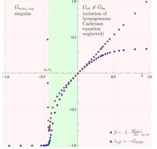
the finite wavefunction renormalisation $(1+\mathcal{Y})$ given by (41). Figure 1 shows both $\mathcal{Y}$ and

the effective coupling constant $\lambda_{eff}$ given by (45)

as

functions of

$\lambda$

. We find clear

Figure 1: $\mathcal{Y},$ $\lambda_{eff}$ based

on

$G_{a0}$ for $\Lambda^{2}=10^{7}$ with

2000

sample points.

evidence for

a

second-order phase transition: $\mathcal{Y}’$ is discontinuous at _{$\lambda_{c}=-0.396,$}

and

we

have in reasonable approximation

a

critical behaviour

for

some

$A,$ $\alpha>0$. To beprecise, we find $1+\mathcal{Y}=0$ only at $\lambda_{0}=-0.455$, but this

seems

to be due to the discretisation. Of course, there cannot be a discontinuity

in $\mathcal{Y}’$ for finite $\Lambda$

, but Figure 1 is strong support for

a

critical behaviour (52) in

the limit $\Lambda^{2}arrow\infty$.

It is

worthwhile

to mention that nothing particular happens

at the expected pole $\lambda_{b}=-\frac{1}{72}=0.014$ of Borel resummation!

Since

$1+\mathcal{Y}=0$

(withinnumerical

error

bounds) inthe phase $\lambda<\lambda_{c}$, we

see

from (44) that higher $N$-point functions will not exist for $\lambda<\lambda_{c}$. Most surprisingly,

as

we discuss at

the end of section 4.2, a key property of the Schwinger 2-point function $S_{c}(x, y)$

in position space is precisely realised in $[\lambda_{c}, 0]$, not outside. To be

more

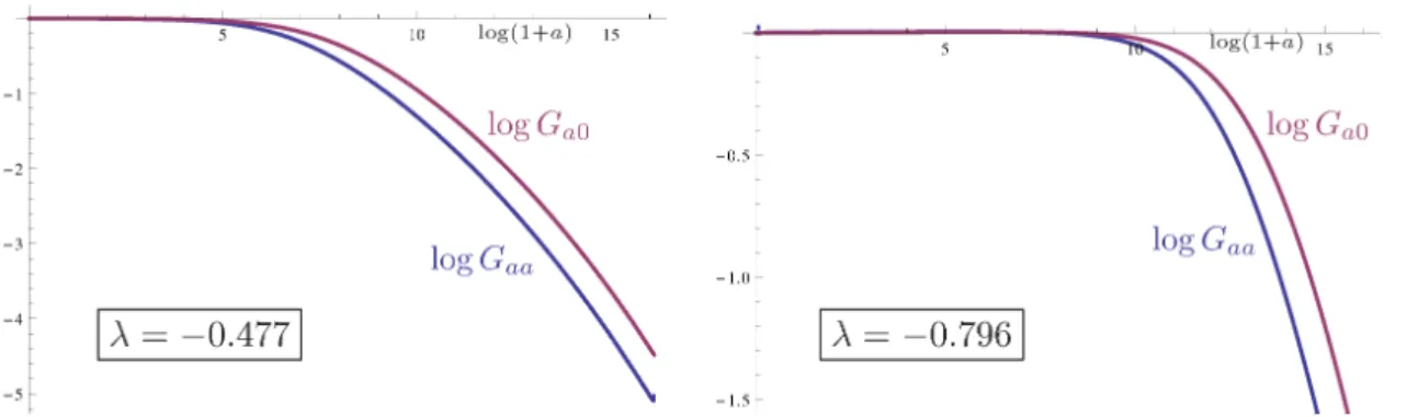
precise, Figure 2 suggests $G_{ab}=0$ for $0\leq a,$$b\leq\Lambda_{0}^{2}$, where $\Lambda_{0}^{2}$ increases with $\lambda_{c}-\lambda>0.$

Figure 2: Plots of $\log G_{a0}$ and $\log G_{aa}$

over

_$\log(1+a)$ for $\lambda<\lambda_{c}.$

This could leave the possibility of meaningful higher functions (44) for matrix indices $0\leq a_{i}\leq\Lambda_{0}^{2}$, but not for larger indices. Such a picture could have the

interpretation of a maximal momentum cut-offof the Euclidean particles.

4

Schwinger

functions

and reflection positivity

In the previous section

we

have constructed the connected matrix correlation

functions $G_{|\underline{q}_{1}^{1}\ldots\underline{q}_{N_{1}}^{1}|\ldots|\underline{q}_{1}^{B}\ldots\underline{q}_{N_{B}}^{B}|}$ of the $(\thetaarrow\infty)$-limit of

$\phi_{4}^{4}$-theory

on

Moyal space.

These

functions

arise from the topological expansion (6) ofthe free energy

$\log\frac{\mathcal{Z}[J]}{\mathcal{Z}[0]}=\sum_{B=11\leq N_{1}}^{\infty}\sum_{\leq\cdots\leq N}^{\infty}\frac{(V\mu^{4})^{2-B}}{BS_{N_{1}\ldots N_{B}}}\sum_{\underline{q}_{i}^{\beta}\in \mathbb{N}^{2}}G_{|\underline{q}_{1}^{1}\ldots\underline{q}_{N_{1}}^{1}|\ldots|\underline{q}_{1}^{B}\ldots\underline{q}_{N_{B}}^{B}|}\prod_{\beta=1}^{B}\frac{1}{N_{\beta}}(\frac{J_{\underline{q}_{1}^{\beta}\underline{q}_{2}^{\beta}}}{\mu^{3}}\cdots\frac{J_{\underline{q}_{N_{\beta}}^{\beta}\underline{q}_{1}^{\beta}}}{\mu^{3}})$.

(53)

Since

$\lim_{V\mu^{4}arrow\infty}G_{|\underline{q}_{1}^{1}\ldots\underline{q}_{N_{1}}^{1}|\ldots|\underline{q}_{1}^{B}\ldots\underline{q}_{N_{B}}^{B}|}$ is finite, the limit $\lim_{Varrow\infty}\frac{1}{V\mu^{4}}\log_{\mathcal{Z}[0]}^{ZJ}\perp$ of the

naturally expected free energy density

removes

(in addition to the removal of higher-genus contributions) all contributions from $B\geq 2$.

As

shown in previous sections, this planar limit is an exactly solvable and (without any doubt)