On the Phase Transition Phenomenon of Graph Laplacian Eigenfunctions on Trees (Recent development and scientific applications in wavelet analysis)

On the Phase

Transition

Phenomenon

of Graph

Laplacian Eigenfunctions

on

Trees

Naoki

Saito

and Emest

Woei

Department of Mathematics

University of Califomia

Davis,

_CA

₉₅₆₁₆

USA

Email: saitoGmath.

ucdavis.

edu;

woei Gmath.

ucdavis.

edu

Abstract

Wediscussourcurrentunderstandingonthephase transition phenomenonof the

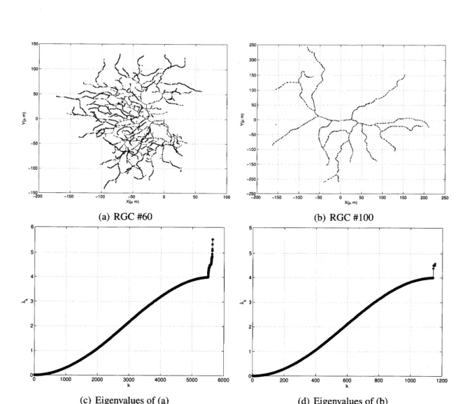
graph Laplacian eigenfunctions constructedon acertaintypeoftrees,whichwe pre-viously observed through our numerical experiments. The eigenvalue distribution for suchatreeisasmoothbell-shaped curvestartingfrom the eigenvalue $0$upto4.

Then, atthe eigenvalue 4,there is a suddenjump. Interestingly, the eigenfunctions

corresponding tothe eigenvalues below 4are semi-global oscillations (likeFourier

modes)overtheentiretree or oneof the branches; on the otherhand, those

corre-spondingtotheeigenvaluesabove 4

are

muchmorelocalizedandconcentmted(like

wavelets) aroundjunctions/branching vertices. For a special class of trees called

starliketrees,wecannow explainsuchphasetransitionphenomenon precisely. For

amorecomplicatedclassof treesrepresentingneuronaldendrites, wehavea

conjec-turebasedonthe numerical evidencethatthenumberoftheeigenvalues largerthan 4is bounded from abovebythe number of vellices whose degrees is strictlylarger

than2. We have alsoidentifiedaspecial classof trees thataretheonlyclass oftrees

thatcanhave the exacteigenvalue4.

1

Introduction

More and

more

data

are

collectedin

a

distributed and irregular

manner

due to the advent

of

sensor

technology. Such data

are

not

so

organized

as

familiar digital signals andimages

sampled

on

regularlattices. Examples include datameasured

on sensor

networks, social

networks, webpages, biological networks, and

so on.

Such unorganized data

can

be

con-veniently represented

as

a

graph where each vertex represents

a

sensor

or

measured data

by

a

sensor

and each edge represents

a

relationship (e.g.,

a

physical

or

wireless

connec-tivity

or a

certain

measure

ofaffinity, etc.) between twoverticesconnectedby that edge.

Moreover, constmcting

a

graph from

a

usual signal

or

image and analyzing it

can

also

leadto

a

very

powerful tool (e.g.,the nonlocal

mean

denoisingalgorithm ofBuades, Coll,

and Morel [1]$)$

.

Hence, it is

very

important to transfer harmonic and wavelet analysis

techniques, which

were

originally developed

on

the usual Euclidean

spaces

and

proven

to graphs and networks. Examples of such effort includes spectral graph wavelet

trans-form of Hammond, Vandergheynst, and Gribonval [8] and the tensor-product Haar-like

basis for digital databases proposed by Coifman, Gavish, and Nadler [3, 5], to

name

just

a

few. As sines, cosines, and complex exponentials play

a

fundamental role in harmonic

analysis

on

the Euclidean

spaces,

thegraph Laplacian eigenfunctions play such

a

role

on

graphs (note that the sines, cosines, and complex exponentials

are

the Laplacian

eigen-functions for

an

interval with the Dirichlet, Neumann, andperiodic boundaryconditions,

respectively). Hence, it isof crucial importance tounderstand the behavior of the graph

Laplacianeigenfunctions of

a

given graph. Inthis shortnote,

we

willdescribe

our

effortto

understand the

surprising

behavior of the graph Laplacian

eigenfunctions

on

treesthat

we

discovered previously[9]:

some

ofthem

are

globaloscillationslikeFourier modes and the

others

are

localizedwiggles likewavelets depending

on

thecorresponding eigenvalues.

In

our

previousreport [9],

we

proposed

a

methodtocharacterize dendritesofneurons,

more

specifically retinalganglioncells(RGCs)of

a

mouse,and cluster them intodifferent

cell typesusingtheirmorphological features, which

are

derived from the eigenvalues of

the graph Laplacians when such dendrites

are

represented

as

graphs (in fact literally

as

“trees”). For the details

on

the dataacquisition andthe conversionof dendrites tographs,

see

[9] and references therein. While analyzing the eigenvalues and eigenfunctions of

those graph Laplacians,

we

observed

a

very

peculiarphase tmnsition phenomenon

as

shown in Figure 1. In otherwords, the eigenvalue distribution for each dendritic tree is

a

smooth bell-shaped

curve

starting from the eigenvalue $0$

up

to 4. Then, at the

eigen-value 4, there is

a

sudden

jump

as

shown

in

Figure

1

$(c, d)$

.

Interestingly, the eigenfunc-tions corresponding tothe eigenvalues below 4

are

semi-globaloscillations (likeFourier

cosines/sines)

over

theentire dendrites

or one

of the dendrite arbors(or branches);

on

the

otherhand, those correspondingtothe eigenvalues above 4

are

much

more

localized

and

concentmted(like wavelets) aroundjunctions/branching vertices,

as

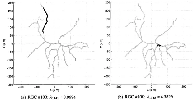
shownin Figure2.

We want to

answer

the followingquestions:

Ql Why does such

a

phase

transition

phenomenonoccur?

Q2 What isthesignificance of the eigenvalue 4?

Q3 Is there

any

treethat

possesses

theexacteigenvalue 4?

At this

point

of time,

we

have

a

complete

answer

to Q3, which will be described

in

Section 5. As forQl andQ2,

we

have

a

complete

answer

for

a

specificandsimple class of

treescalled starliketreesasdescribed in Section3,and apartial

answer

for

more

general

trees such

as

those representingneuronal dendrites, which

we

will discuss in Sections 4

and6.

2

Definitions and Notation

Let $G$ be

a

graph representing dendrites of

an

RGC, and let $V(G)=\{\nu_{1}, \nu_{2},\ldots, \nu_{n}\}$ be

a

setofvertices in $G$where each $\nu_{k}\in \mathbb{R}^{3}$represents

a

sampled point(in the $3D$ coordinate

system) along dendritic arbors of this RGC. Let $E(G)=\{e_{1},e_{2},\ldots,e_{m}\}$ be

a

set of edges

where $e_{k}$connectstwo

vertices

$\nu_{i},$$\nu_{j}$ for

some

$1\leq i,j\leq n$,and

we

write$e_{k}=(v_{i}, \nu_{j})$

.

Let

$-200$ $-150$ - $t$00 $X(\mu m)-50$ $0$ (a) RGC#60 50 $t00$ $0$ 1000 2000 _{3000 4000 5000 6000} $0$ 200 400 600 800 1000 1200 $k$ $k$

(c) Eigenvalues of(a) (d) Eigenvalues of(b)

Figure 1: Typical dendrites of Retinal Ganglion Cells (RGC) of

a

mouse

and the graph

Laplacian eigenvalue distributions. (a) $2D$ projection ofdendrites of RGC of

a

mouse;

(b) _{that of another RGC revealing different morphology;} (c) the eigenvalue distribution

ofRGC shown in (a); (d) that of RGC shown in (b). Regardless of their morphological

X$(\mu m)$

(a) RGC #100;$\lambda_{1141}=3.9994$

$X(\mu m)$

(b) RGC #100;$\lambda_{1142}=4.3829$

Figure

2:

Thegraph Laplacian eigenfunctions of RGC

#100.

(a)The

one

correspondingto the eigenvalue $\lambda_{1141}=3.9994$, immediately below the value4; (b) the

one

corresponding

tothe eigenvalue$\lambda_{1142}=4.3829$, immediately abovethevalue 4.

can

be convertedto

a

tree rather than

a

general graph since it is connected and contains

no

cycles;

see

[9] forthedetails. We alsonote that

we

only deal with unweighted graphs

in this

paper.

In other words,

we

essentially examine the connectivities, topology, and

complexity ofthe dendritic trees, which

may

not reflect the physical lengths andwidths

of the dendritic arbors;

we

are

currently investigatingweightedgraphs where the weights

are

related to the physical distances between vertices, and hope that

we

can

report

our

findingsat

a

later date. Let $L(G);=D(G)-A(G)$ be the (combinatorial)Laplacian matrix

where$D(G);=$diag$(d_{\nu_{1}},\ldots,d_{\nu_{n}})$iscalled the degreematrix of$G$, i.e.,the diagonalmatrix

ofvertex degrees, and $A(G)=(a_{ij})$ is the adjacency matrix of $G$, i.e., _{$a_{ij}=1$} if $\nu_{i}$ and $\nu_{j}$

are

adjacent; otherwise it is

$0$

.

Furthermore, let $0=\lambda_{0}(G)\leq\lambda_{1}(G)\leq\cdots\leq\lambda_{n-1}(G)$be

the sorted eigenvalues of$L(G)$

.

Let $m_{G}(\lambda)$ be themultiplicity of the eigenvalue $\lambda$

.

More

generally, if$I\subset \mathbb{R}$ is

an

interval of the realline, then

we

define $m_{G}(I);=\#\{\lambda_{k}(G)\in I\}$

.

At this

point

we

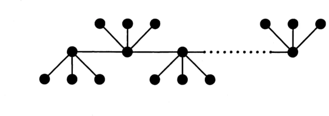
would like to give

a

simple yet

important

example of

a

tree and

its

graph Laplacian:

a

path graph consisting of $n$

vertices

shown in Figure

3.

The graph

Laplacian of such

a

pathgraph

can

beeasily obtained andis instructive.

$L(G)$ $=$ $D(G)-A(G)$

$\{\begin{array}{llllll}l -l -l 2 -l -l 2 -l \ddots \ddots \ddots -l 2 -l -l l\end{array}\}$ $=$ $\ovalbox{\tt\small REJECT}^{1}$

2

2

...

2

$1\ovalbox{\tt\small REJECT}-\ovalbox{\tt\small REJECT}^{0}1$

$011$

$01$

. $11$

.

$01^{\cdot}$ $01\ovalbox{\tt\small REJECT}$

.

The

eigenvectorsl

of this matrix

are

nothing but the $DCT$TypeIIbasis vectors used for

theJPEG image compression standard;

see e.g.,

[10]. In fact,

we

have

$\lambda_{k}=2-2\cos(\pi k/n)=4\sin^{2}(\pi k/2n),$ _{$k=0,1,\ldots,$$n-1$};

$( \rho_{k}=(\cos(\pi k(j+\frac{1}{2})/n))_{0\leq j<n}^{T},$ $k=0,1,\ldots,$$n-1$.

Note that for

any

finite $n\in \mathbb{N},$ $\lambda_{\max}=\lambda_{n-1}<4\neq$, and

no

localization/concentration

occurs

in the eigenvector $\phi_{n-1}$, which is simply

a

global oscillation with the highest possible

(i.e.,the Nyquist)frequency, i.e., $\phi_{n-1}=((-1)^{j}\sin(\pi(j+\frac{1}{2})/n))_{0\leq j<n}^{T}$

.

3

Analysis of

Starlike Trees

As

one can

imagine, analyzing this phase transition phenomenon for complicated

den-dritic treestums outtoberather difficult. Hence,

we

start

our

analysis

on a

simpler class

oftreescalled starliketrees. A starliketree is

a

treethat has exactly

one

vertex of degree

greater than 2. Examples

are

shown in Figure 4. We

use

the following notation. Let

(a) $S(2,2,1,1,1,1)$ (b) $S(n_{1},1,1,1,1,1,1,1)$ a.k.a.comet

Figure4: Typical examples of

a

starlike tree.

$S(n_{1}, n_{2},\ldots, n_{k})$ be

a

starliketreethat has $k(\geq 3)$paths (i.e., branches)emanatingfrom the

central vertex $\nu_{1}$

.

Let the $i$thbranch have $n_{i}$ verticesexcluding $\nu_{1}$

.

Let $n_{1}\geq n_{2}\geq\cdots\geq n_{k}$

.

Hence,the total number ofvertices is $n=1+ \sum_{i=1}^{k}n_{i}$

.

Soon after

we

proved in

2010

the largest eigenvalue for

a

comet (a special class of

starlike trees

as

shown in Figure 4 $(b))$ is always larger than 4,

we

noticed the following

more

general results for

any

starlike treeobtainedby Das in

2007

[4]:

$\lambda_{\max}=\lambda_{n-1}<k+1+\frac{1}{k-1}$; (1)

$2+2 \cos(\frac{2\pi}{2n_{k}+1})\leq\lambda_{n-2}\leq 2+2\cos(\frac{2\pi}{2n_{1}+1})$

.

(2)

On the otherhand, Grone and

Merris

[6] proved the followinglowerbound for

a

general

graph $G$withatleast

one

edge:

$\lambda_{\max}\geq\max_{1\leq j\leq n}d(\nu_{j})+1$

.

(3)

Hence

we

have the following

Corollary

3.1.

A starlike tree has exactly

one

gmph Laplacian eigenvalue greaterthan

orequalto 4. The equality holds$\iota f$and only

if

the starliketree is$K_{1},3=S(1,1,1)$, which is

also knownas$a$claw.

Pmof.

Thefirst statementis

easy

to show. The lowerbound in(3) is larger than

or

equal

to4for

any

starliketreesince$\max_{1\leq j\leq nj}d(\iota/)=d(\nu_{1})\geq 3$

.

On the otherhand,the second

largest eigenvalue $\lambda_{n-2}$ clearly cannot exceed 4 due to (2). The second statement about

the

necessary

and sufficient condition

on

the equality requiresthe argument in Section5, in particular,Corollary

5.2.

Fromthis,

we

can

easily

see

that the only starliketreehaving theexacteigenvalue4is$K_{1}$_,3.

$\square$

As for the concentration/localization _{ofthe eigenfunction} $\phi_{n-1}$ correspondingto the

largest eigenvalue $\lambda_{n-1}$,

very

recently

we

haveprovedthe following

Theorem

3.2.

Let $\phi_{n-1}=$ $(\phi_{1,n-1}, \cdots ,\psi_{n,n-1})^{T}$, where $\phi_{j,n-1}$ is the value

of

the

eigen-function

corresponding to the largesteigenvalue $\lambda_{n-1}$at thevertex $\nu_{j},$ $j=1,\ldots,$$n$

.

Then,

the absolute value

_of

this eigenfunction at the centml vertex $\nu_{1}$ cannot be exceededby

thoseatthe othervertices, i.e.,

$|\phi_{1,n-1}|>|\phi_{j,n-1}|$, $j=2,\ldots,$$n$

.

Thedetails oftheproof will

appear

elsewhere. We note that Dasprovedthis theorem

for

a

homogeneous starlike tree, $S(m, m,\cdots , m)$ in [4], and

our

theorem isfor

a

general

starliketree.

Remark

3.3.

Let $\phi=(\phi_{1},\phi_{2},\ldots,\phi_{n})^{T}$be

an

eigenvector of

a

starlike tree $S(n_{1},\ldots, n_{k})$

corresponding to the eigenvalue $\lambda$

.

Let

$\nu_{2},\ldots,$ $\nu_{n_{1}+1}$ be the $n_{1}$ vertices along

a

branch

emanating from the central vertex $\nu_{1}$ with $\nu_{n_{1}+1}$ being the leaf vertex. Then, along this

branch,theeigenvectorcomponents satisfy the followingequations:

$\lambda\phi_{n_{1+1}}$ $=$ $\phi_{n_{1}+1}-\phi_{n_{1}}$ (4)

From Eq. (5),

we

have the followingrecursion relation:

$\psi_{j+1}+(\lambda-2)\phi_{j}+\phi_{j-1}=0$, $j=2,\ldots,$$n_{1}$

.

(6)

This recursion

can

be explicitly solvedusingthe rootsof thecharacteristic equation

$r^{2}+(\lambda-2)r+1=0$_{, (7)}

andthegeneral solution

can

be

written

as

$\phi_{j}=Ar_{1}^{i-2}+Br_{2}^{i-2}$, _{$j=2,\ldots,$}$n_{1}+1$, (8)

where $r_{1},$$r_{2}$

are

the roots of (7), and $A,B$

are

appropriate constants derived from the

boundary condition (4). Now, let

us

consider these roots of (7) in details. The

deter-minantof(7)is

$\prime D(\lambda);=(\lambda-2)^{2}-4=\lambda(\lambda-4)$

.

₍₉₎

Since

we

know that $\lambda\geq 0$, this determinant changes itssign depending

on

$\lambda<4$

or

$\lambda>4$.

(Note that $\lambda=4$

occurs

only for the claw $K_{1,3}$

on

which

we

explicitly know everything;

hence

we

will notdiscuss this

case

further in this remark.) _If$\lambda<4$_, then $\prime D(\lambda)<0$ andit

is

easy

toshowthat theroots

are

complex valued with magnitude 1. This implies that (6)

becomes

$\phi_{j}=A’\cos(\omega(j-2))+B’\sin(\omega(j-2))$_, $j=2,\ldots,$$n_{1}+1$, (10)

where$\omega$ satisfies$\tan\omega=\sqrt{\lambda(4-\lambda)}/(2-\lambda)$, and$A’,B’$

are

appropriateconstants. In other

words, if$\lambda<4$, the eigenfunction along this branchis of oscillatorynature. On the other

hand, if $\lambda>4$, then $D(\lambda)>0$ and it is easy to show that both $r_{1}$ and $r_{2}$

are

real valued

that the dominating partis theterm $Br_{2}^{i-2}$ in (8). The siuation is the

same

for the other

branches. This observation has lead

us

to the proof of Theorem 3.2, which

we

deferto

our

forthcoming

paper.

In

summary,

for

a

starlike tree, thephase transitionphenomenon

with the eigenvalue4 is hence essentially explained andwellunderstood.

4

Our Conjecture

Unfortunately, actual dendritic trees

are

not exactly starlike. However,

_our

_numerical

computations anddata analysis indicate that:

$0 \leq\frac{\#\{j\in(1,n)|d(\nu)>2\}-m_{G}([4,\infty))}{n}\leq 0.047$ ₍₁₁₎

foreach RGC

we

examined. Hence,

we can

define starlikeliness $S\ell(T)$ of

a

giventree $T$

as

$S \ell(T):=1-\frac{\#\{j\in(1,n)|d(\iota_{j\neq}/)>2\}-m_{T}([4,\infty))}{n}$ ₍₁₂₎

We note that $SP(T)\equiv 1$ for

a

certain class of RGCs whose dendrites

are

widely and

sparsely spread (see [9] forthe characterization). This

means

that dendrites inthat class

are

all close to

a

starlike tree

or a

concatenation of several starlike trees. We show

some

examples of

dendritic

trees with $Sl(T)\equiv 1$ andthose with $Sl(T)_{\neq}<1$ in Figures 5, 6, and

7.

Cell$\#$$99$ Cell$\#$_$100$ $-50$ $0$ 50 Cell$\# 101$ $-100$ $-50$ $0$ 50 100 150 Cell$\# 196$ $-200$ _-loo 0100 200 Cell$\# 210$ $-50$ $0$ 50 $-100$ $0$ 100 Cell$\# 102$ $-150$ $-100$ $-50$ $0$ 50 Cell$\# 201$ $-200$ $0$ 200 $400$ Cell$\# 174$ $-200$ $0$ 200

$-40$ $-20$ $0$ 20 40 Cell$\# 166$ $-40$ $-20$ $0$ 20 40 60 Cell$\# 238$ $-40$ $-20$ $0$ 20 40 Cell$\# 215$ $-60$ $-40$ $-20$ $0$ 20 40 $-40$ $-20$ $0$ 20 Cell$\# 80$ $-50$ $0$ 50 Cell$\# 169$ $-60$ $-40$ $-20$ $0$ 20 Cell$\# 55$ $-100$ $-50$ $0$ 50 100

X$(\mu m)$

(a) RGC #100;$S\ell(T)\equiv 1$

$X(\mu m)$

(b) RGC #155;$Sl(T)=0.953\lessgtr 1$

Figure7: Zoomed-upversionsof

some

dendritic trees.

Conjecture

4.1.

For

any

tree $T$

offinite

volume,

we

have

$0\leq m_{T}([4,\infty))\leq\#\{j\in(1, n)|d(\nu_{l^{)}\neq}>2\}$

and each eigenfunction correspondingto$\lambda\geq 4$hasits largestcomponent(in theabsolute

value)

on

the vertices whose degree

are

largerthan2.

5

A Class of Trees Having the Eigenvalue

4

As raised in Introduction,

we are

interested in answering Q3: Is there

any

treethat

pos-sesses

theexact eigenvalue 4? To

answer

this question,

we

have recently found that the

following resultsofGuo [7] (written in

our own

notation):

Theorem

5.1

(Guo 2006). Let $T$ be

a

tree with $n$ vertices. Then,

$\lambda_{j}(T)\leq\lceil\frac{n}{n-j}\rceil$, _{$j=0,\ldots,$}$n-1$,

and theequalityholds

_iff

$a$) $j\neq 0;b)n-j$ divides $n$; andc) $T$ is spanned by $n-j$ vertex

disjointcopies

_of

$K_{1.\frac{j}{n-i}}$.

This impliesthefollowing

Corollary

5.2.

Atreethat has

an

eigenvalue exactlyequalto 4necessarilyconsists

_of

$m$

copies

_of

$K_{1},3\equiv S(1,1,1)$ connectedvia theircentmlvertices

as

shown in Figure8 where

$m\in \mathbb{N}$

.

Pmof.

Set $n=4m$ in Guo’s theorem. Then, there is

an

eigenvalue exactly equal to 4 at

$j=3m$ , i.e., $\lambda_{3m}=4$, and this tree necessarily consists of $m$ copies of $K_{1}$

,3 connected

via their central vertices, which is guaranteed because of the

necessary

and sufficient

Figure 8: Atreeconsistingof multiplecopiesof$K_{1,3}$ connectedviatheir central vertices.

Thistree has theexacteigenvalue4with multiplicity 1.

Figure

9

showstheeigenvalue distributionof

a

treeconsisting of$m=5$

copies

of$K_{1}$_,3.

Regardless of $m$, the number of

copies

of$K_{1,3}$, the eigenfunction corresponding to the

eigenvalue 4 has onlytwovalues:

one

constantvalue atthe central vertices, and the other

constantvalueof theopposite signatthe leaves whereas that correspondingtothe largest

eigenvalue is againconcentrated around the central vertex,

as

shownin Figure 10.

6 Discussion

In this

paper, we

obtained precise understanding ofthe phase transition phenomenon of

the graph Laplacian eigenvalues and eigenfunctions for starlike trees. For

a more

com-plicated class oftrees representingdendrites ofRGCs,

we

obtained

a

conjecturebased

on

the numerical evidence that the number of the eigenvalues larger than 4 is bounded from

above bythe number ofvertices whosedegrees is strictlylarger than 2. We also identified

a

special class of trees consisting ofcopies of the claw $K_{1}$_,3, which is the only class of

treesthat

can

have theexacteigenvalue 4.

Ournextstep toward understanding the phasetransitionphenomenon for real dendritic

trees is to analyze

a

slightly

more

complicated class of trees, i.e., trees generated by

concatenating several starlike trees. Since

we now

know the eigenvalue/eigenfunction

behavior of starliketreesprecisely,

we

expectthat

we

can

also shedlight

on

that class of

trees. Weplantoproceed such analysis bystarting withtwo concatenated starliketrees.

Another quite interesting question is the following. Can

a

simple (i.e.,

no

multiple

edges and

no

self-loops) and connected graph–not necessarily

a

tree–have the exact

eigenvalue 4? The

answer

isclear “Yes.” For example,

a

regular finite lattice graph in$\mathbb{R}^{d}$

,

$d>1$ _{has repeated eigenvalue 4. Moreprecisely, each eigenvalue and the corresponding}

eigenfunction of

a

graphrepresentingthe regularfinite lattice ofsize $n\cross n\cross\cdots\cross n=n^{d}$

can

bewritten

as

$\lambda_{j_{1\cdots\prime}j_{d}}$ $=$

$\phi_{j_{1},\ldots,j_{d}}(x_{1},\ldots,x_{d})$ $=$

4$\sum_{i=1}^{d}\sin^{2}(\frac{j_{i}\pi}{2n}1$ (13)

Figure9: The eigenvaluedistributionof

a

treeconsisting of 5 copiesof$K_{1.3}$

.

Wenote that

(a) $\psi_{15}$

(b) $\psi_{19}$

Figure 10: (a)_{The eigenfunction} $\phi_{15}$ correspondingto $\lambda_{15}=4$of the tree 5$K_{1,3}$ inthe$3D$

perspective view. (b) Theeigenfunction $\phi_{19}$ corresponding to the maximumeigenvalue

where $j_{i},x_{i}\in Z/nZ$for each $i$,

as

shown by Burden and Hedstrom [2]. Hence,

determin-ing $m_{G}(4)$, i.e., the multiplicity of the eigenvalue 4 of this lattice graph, isequivalent to

finding theinteger solution $(j_{1},\ldots,j_{d})\in(Z/nZ)^{d}$ tothe followingequation:

$\sum_{i=1}^{d}\sin^{2}(\frac{j_{i}\pi}{2n})=1$

.

(15)

For$d=2$, it is

easy

toshow that $m_{G}(4)=n-1$ by direct examination of(15) with $d=2$

.

For $d=3,$ $m_{G}(4)$ behaves in

a

much

more

complicatedmanner, which is deeply related

to number theory. We expect that

more

complicated situations

occur

for $d>3$

.

We

are

currently investigatingthis interesting problem

on

regular finite lattices with Yuji

Nakat-sukasa ofUC Davis, and

we

plan toreport

our

findings at

a

laterdate. Onthe otherhand,

it is clearfrom (14)that the eigenfunctions correspondingto the eigenvalues greater than

or

equalto 4

on

such lattice graphs cannotbe localized

or

concentrated

on

those

vertices

whosedegree is larger than 2 unlike thetree

case.

References

[1] A. BUADES, B. COLL, AND J. M. MOREL,Image denoisingmethods.A

new

non-local principle, SIAMReview, 52 (2010),

pp. 113-147.

[2] R. L. BURDEN AND G. W. HEDSTROM, The distribution

of

the eigenvalues

of

the

discrete Laplacian, BIT, 12(1972),

pp.

475-A88.

[3] R. R. COIFMAN AND M. GAVISH, Harmonic analysis

_of

digital data bases, in

Wavelets andMultiscale Analysis: Theory and Applications,J. Cohenand A. Zayed,

eds., Applied and Numerical HarmonicAnalysis, Boston, MA, 2011, Birkhauser.

[4] K.C.DAS,Some spectml pmperties

_of

the Laplacian matrix

_of

starliketrees,Italian

J. PureAppl. Math.,

21

(2007),

pp.

197-210.

[5] M. GAVISH, B. NADLER, AND R. R. COIFMAN, Multiscale wavelets

on

trees,

graphs and high dimensional data: theory and applications to semi

super-vised leaming, in Proc. 27th Intem. Conf. Machine Leaming, J. F\"urnkranz _and

T.Joachims, eds., Haifa, Israel, 2010,Omnipress,

pp. 367-374.

[6] R. GRONE AND R. MERRIS, The Laplacian spectrum

_of

a

graphII, SIAMJ.

Dis-creteMath.,7 (1994),pp. 221-229.

[7] J.-M. GUO, The kth Laplacian eigenvalue

_of

a

tree, J. Graph Theor., 54 (2006),

pp.

51-57.

[8] D. K. HAMMOND, P. VANDERGHEYNST, AND R. GRIBONVAL, Wavelets on

graphs via spectml gmph theory, Applied and Computational Harmonic Analysis,

(2011). To

appear;

available online

as an

in-press itematwww.sciencedirect.com.

[9] N. SAITO AND E. WOEI,Analysis

_of

neumnal dendritepattemsusing eigenvalues

of

graph Laplacians,JSIAMLetters, 1 (2009),

pp.

13-16. Invited

paper.