Russian Options with Finite Time Horizon: A Laplace Transform Approach(Mathematics in a Decision Making with Uncertainties and Its Applications)

Russian

Options with Finite

Time

Horizon:

A Laplace Transform

Approach*

北海道大学・経済学研究科 木村俊一 (Toshikazu Kimura)

Graduate School of Economics and Business Administration

Hokkaido University

1

Introduction

Russian options

are

path-dependent contingent claims that give the holder the right to receive

the realized supremumvalue of the underlying asset prior to his exercise time. The holder

can

exercise the option atany tinle, $i.e.$, the option is of American-style. Shepp and Shiryaev $[12, 13]$

introduced the Russian option, $ab^{\neg}suming$ no maturity date for the exercise; see Duffie and

Harrison [3] for afinancialjustification of their result8. Shepp and Shiryaev showed that there

exists

an

optimal threshold level of theasset price below which it isadvantageous toexercise the

option, provided that the asset pays dividends. This type of Russian options

can

be regarded

as

aspecial

case

of

American

lookbackoptions. More specifically, it is the perpetual fixed-strike

lookback call option wlth null strike price(Pedersen [10]). In

common

with lookback options,

Russian options are not genuine option contracts, because they pay the holder the supremum

Isset price, always finishing in-the-money. This

means

that high premiums

are

charged for

Russian optiollS in compensation $fo\iota\cdot$ “reduced

$1^{\cdot}Cgl\cdot et’[12]$

.

This paper deals with Russian options $wit1_{1}fir\iota iteti_{7}nehor^{v}izon,$ $i.c.$, there is afinite $expi_{1}\cdot y$

or maturity date for the exercise. Thc holder lnay $exelcis^{1}e$ the option at any time but durillg

the option’slifetinle. Recently,

some

$\iota\cdot esearchelS$ have $contrib_{l1}ted$ theoretical results to the

valuation of finite-lived Russian options. $Ekst_{1}\cdot\ddot{o}m[5]$ showed $t1_{1}e$ existence and continuity of

an optimal stopping or early $exe7cise$ boundaly for the Russian option. Also, Ekstr\"om proved

that the option value is given by the solution ofacertain boundary value problem, from which

he analyzed asymptotic behavior of the optimal stopping boundary

near

expiration. This free

boundary $p_{1}\cdot oblem$

was

$furt1_{1}er$ studied by Duistermaat et al. [4] who suggested anumerical

algorithm for valuing the Russian option;see Kyprianou and Pistorius [9] for related thmretical

wolk. Peskir [11] provedthat the $opti_{1}\cdot na1$stoppingboundary

can

becharacterized by the solution

of anonlinear integral equation arising $fi\cdot om$ the early $exel\cdot cise$ prelnium representation.

Except for Duisterm’aat et al. [4], there is no quantitative researdl of the finite-lived Russian

option, whichis$\iota$)$rinci_{I)}ally$due to thelackof efficienttools$fo1^{\cdot}$solving the$hee$boundary probleIn.

Duistermaat et al. [4] have used the Imethod of randomization of Carr [2] $w\mathfrak{l}_{1}o$ proposed that the

value ofan American vanilla option can be approximated by arandomization of the maturity

date using

an

$n$-stage$E_{1}\cdot 1angian$distribution. As$narrow\infty$, it ispossibletoshowconvergenceto the

value of theAnlericanoption. Thisidea has its origin in the classictheory of integraltransforms,

and it goes by the

name

of the Post-Widder inversion formula [15];

see

Abate and Whitt [1,

Section

8]

for

all algorithm based

on

theFourier$se_{\wedge}\cdot ies$

.

Duistermaat

et al. developed alecursive

$alg_{o1^{\backslash }}ithm$ for computing the n-th approximations ofthe val

$ne$ and the early exercise boundary

of the finlte-lived Russian option. The complexity of$thci\iota\cdot algo\iota\cdot ith_{l}ncome_{\backslash };$ flom the $\exp_{1}\cdot ession$

of the $n$-stage Erlangial) $dist_{1}\cdot ibution$, and it is _{$dil\cdot ectlyCOl$)}$CC\Gamma lucd$ with the implementation and

speed of the algorithm. The $p_{\mathfrak{U}1}\cdot po_{\backslash }\backslash e$ of $this^{\neg}$ paper is to $p_{1}\cdot ovide$ another quantitative method

for colnputing both $t1_{1}e$ option value and the early exelcise boundary.

’This paper is an abbreviated version of Kimura [8]. All proofs, remarks and .gome _{computational results}

areomitted due tothe page restriction. This research was supported $i_{11}$ part by theGrant-in-Aid for Scientific

2

Basic

Framework

2.1

Optimal

stopping

problem

The setup is the standard Black-Scholes-Merton framework where the price of the underlying

asset evolves accordingto ageometric Brownian motion: Let $(S_{t})_{t\geq 0}$ be the price process ofthe

underlying

as

set, which is defined by

$S_{t}=s$exp$\{r-\delta_{f}^{1}\sigma^{2})t+\sigma W_{t}\}$ , $t\geq 0$, (2.1)

where$S_{0}=s>0,$$r>0$istherisk-free rateof interest,$\delta\geq 0$ is the continuous dividend rate,$\sigma>$

$0$ is the volatility coefficient of the asset price, and _{$W\equiv(W_{t})_{t\geq 0}$} is a one-dimensional

standard

Brownian motion process

on

a filtered probabilityspace $(\Omega, \mathcal{F}, (\mathcal{F}_{t})_{t\geq 0}, \mathbb{P})$

.

The filtration $F\equiv$

$(\mathcal{F}_{t})_{t\geq 0}$ is

a

natural

one

generated by $W$ and the probability

measure

$\mathbb{P}$ is chosen

so

that the

stock has

mean

rate of return $r$

.

For the price process $(S_{t})_{t\geq 0}$ and a constant $m\geq s$, define the

supremum process

as

$M_{t}=m \vee\sup_{0\leq u\leq t}S_{u}$, $t\geq 0$, (2.2)

where $a \vee b=\max\{a, b\}$

.

Given

a

finite time horizon $T>0$, the arbitrage-free value of the Russian option at time

$t\in[0,T]$ is given by

$V(s,m, t)=e ss\sup_{0\leq\theta\iota\leq T-t}E_{s,m}[e^{-r\theta}{}^{t}M_{\theta_{t}}]$, (2.3)

where $\theta_{t}$ is a stopping time of the filtration $F$ and the conditional expectation _{$E_{s,m}[\cdot]\equiv$}

$E[\cdot|\mathcal{F}_{0}]=E[\cdot|S_{0}=s, M_{0}=m]$ is calculated under therisk-neutral probability

measure

P. The

randomvariable$\theta t\in[0, T-t]$ iscalled

an

optimal stoppingtime if$V(s, m, t)=E_{s,m}[e^{-r\theta_{t}}M_{\theta_{t}}\cdot]$

.

It is clear from $(2.1)-(2.3)$ _that $V(s, m, t)\geq rn,$ $V$ is nondecreasing in $s$ and $m$, and $V$ is

non-increasing in $t$. Ekstr\"om [5] proved that the value function

$V\equiv V(s, m, t)$ is continuous, $i.e.,$ $V$

is uniformly continuous in $s,$ $m$ and $t$ separately. Solving the optimal stopping problem (2.3) is

equivalent

to

finding the points $(S_{t}, \Lambda l_{t}, t)$ for which early exercise before maturity is optimal.

Let

$\mathcal{D}=\{(s, m, t)\in \mathbb{R}+\cross[s, +\infty)x[0, T]\}$

be the whole domain, and $\mathcal{E}$ and _$C$ denote

the exercise region and continuation region,

respec-tively. In terms of the value function$V(s, m, t)$, _{the continuation region}$C$ is defined by

$C=\{(s, m,t);V(s, m, t)>m\}$,

which is an open set since $V$ is continuous. The exercise region $\mathcal{E}$ is the complement of

$C$ in $\mathcal{D}$

and the optimal stopping time $\theta_{t}^{*}$ satisfies

$\theta_{t}^{*}=\inf\{u\in[0,T-t];(S_{u}, M_{u}, t+u)\in \mathcal{E}\}$

.

Since $V$ is nondecreasing in _{$s,$ $(s, m, t)\in C$} implies _{$(x, m, t)\in C$} for all $x$ satisfying _{$s\leq x\leq m$}

.

Hence, there exists

a

function $\underline{S}(m, t)$ with $0\leq\underline{S}(m, t)\leq m$ such that

$\underline{S}(m,t)=\inf\{s\in[0, m];(s, m, t)\in C\}$, (2.4)

and $(\underline{S}(m, t))_{t\in[0,T]}$ is called the early exercise boundary. The boundary function $\underline{S}(m, t)$ is

nondecreasing in $t$since $V$is nondecreasingin$t$, and it is continuous in $t$ if$\delta>0$;

see

Theorem 2

in Ekstr\"om [5]. In terms of the function $\underline{S}(m, t)$, the continuation region $C$

can

be represented

as

2.2

Free boundary

problem

It has been known that the optimal stopping problem (2.3) of finding the option value $V$

can

be deduced to

a

parabolic free boundary problem (see Theorem 1 in Ekstr\"om [5]): The value $V$

of the Russian option with finite time horizon is given byasolution of the PDE

$\frac{\partial V}{\partial t}+\frac{1}{2}\sigma^{2}s^{2}\frac{\partial^{2}V}{\partial s^{2}}+(r-\delta)s\frac{\partial V}{\partial s}-rV=0$

, $\underline{S}(m.t)<s\leq m$, (2.5)

together withthe boundary conditions

$|m \downarrow s\lim\lim_{s\downarrow\underline{S}}\frac{\partial V}{\frac{\partial V\partial s}{\partial m}}=0\lim V(s,m, t)=ms\downarrow\underline{S}=0’,$

(2.6)

and the terminal condition

$V(s,m, T)=m$

.

(2.7)

The boundary conditions in (2.6)

are

_{respectively called the value matching, smooth pasting and}

Neumann conditions in order.

Fkom (2.3),

we

see

that thevalue $V$ depends

on

timeonly through the time _$T-t$ remaining

to maturity. For notational

convenience. we

introduce the time-reversed quantities

$\tilde{V}(s, m,\tau)=V(s, m, T-\tau)=V(s, m, t)$_,

and

$\tilde{\underline{S}}(m,\tau)=\underline{S}(m,T-\tau)=\underline{S}(m, t)$,

with the change of variables $\tau$ $:=T-t$

.

It follows from the definition (2.3) of the value function

$V$ that

$\tilde{V}$

($ks$, km,$\tau$) $=k\tilde{V}(s, m,\tau)$, (2.8)

for arbitrary $k\in \mathbb{R}+\cdot$ In particular, if

we

set $k=m^{-1}$

,

then

$\overline{V}(s, m, \tau)=m\tilde{V}(\frac{s}{m}, 1,\tau)$

,

which permits a reduction in the dimensionality of the problem by a similarity variable. That

is,

we

may find

a

solution of the form

$\tilde{V}(s, m, \tau)=mW(\xi,\tau)$, _(2.9)

with the change of variables $\xi:=s/m$

.

Using the relations

$\frac{\partial V}{\partial s}=\frac{\partial W}{\partial\xi}$, $\frac{\partial^{2}V}{\partial s^{2}}=\frac{1}{m}\frac{\partial^{2}W}{\partial\xi^{2}}$

$\frac{\partial V}{\partial m}=W-\xi\frac{\partial W}{\partial\xi}$, $\frac{\partial V}{\partial t}=-m\frac{\partial W}{\partial\tau}$,

we

can

rewrite the PDE (2.5)

as

$- \frac{\partial W}{\partial\tau}+\frac{1}{2}\sigma^{2}\xi^{2}\frac{\partial^{2}W}{\partial\xi^{2}}+(r-\delta)\xi\frac{\partial W}{\partial\xi}-rW=()$ ,

where $\underline{\xi}(\tau)(\in[0,1])$ is defined by

$\xi(\tau)=\frac{1}{m}\tilde{\underline{S}}(m, \tau)$,

being nonincreasing in $\tau$. The boundaryconditions for $W$ are given by

$| \xi\downarrow\underline{\xi}(\tau)^{\frac{\partial W}{\partial\xi}=0}\lim_{\xi\uparrow 1}^{\lim^{\lim}}(W-\frac{\partial W}{\partial\xi’})=0\xi\downarrow\underline{\xi}(\tau)W(\xi,\tau)=1$

,

(2.11)

and the initial condition is

$W(\xi, 0)=1$

.

_(2.12)

3

Valuation with

Laplace-Carlson

Transforms

For $\lambda>0$, define the Laplace-Carlson transform (LCT) of the time-reversed quantity $W(\xi, \tau)$

as

$W^{*}( \xi, \lambda)=\mathcal{L}C[W(\xi, \tau)](\lambda)\equiv\int_{0}^{\infty}\lambda e^{-\lambda\tau}W(\xi, \tau)d\tau$

.

Similarly, we denote the LCT of $\xi(\tau)$ by attaching the asterisk, $i.e.,$ $\underline{\xi}^{*}(\lambda)=\mathcal{L}C[\xi(\tau)](\lambda)$

.

No

doubt,

there

is

no

essential difference between the

LCT

and

the

Laplace transform (LT) defined

by

$\overline{W}(\xi, \lambda)=\mathcal{L}[W(\xi, \tau)](\lambda)\equiv\int_{0}^{\infty}e^{-\lambda\tau}W(\xi, \tau)d\tau$

.

Obviously,

we

have $W$“$(\xi, \lambda)=\lambda\overline{W}(\xi, \lambda)$ for $\lambda>0$

.

The principal

reason

why

we

prefer LCTs

to LTs is that LCTs generate relatively simpler formulas than LTs for option pricing problems

because constant values

are

invariant after taking transformation. In the context of option

pricing, LCTs have been adopted in the randomization of Carr [2] as an initial approximation.

Let $\tilde{V}^{*}\equiv\tilde{V}$“_{$(s, m, \lambda)=\mathcal{L}C[\tilde{V}(s, m, \tau)](\lambda)$}

be the LCT of the time-reversed value $\tilde{V}$

.

Hlrom

thePDE (2.10) with the conditions (2.11) and (2.12),

we

obtain

a

closed-formsolution

as

follows:

Theorem 1 The LCT of the time-reversed value $\tilde{V}(s, m, \tau)$ of the Russian option with finite

time horizon $T<\infty$ is given by

$\tilde{V}^{*}(s, m, \lambda)=\{\begin{array}{ll}\frac{mr}{\alpha_{2}-\alpha_{1}\lambda+r}\{\alpha_{2}(\frac{s}{m\underline{\xi}^{*}})^{\alpha_{1}}-\alpha_{1}(\frac{s}{m\underline{\xi}^{*}})^{\alpha_{2}}\}+\frac{\lambda m}{\lambda+r}, m\underline{\xi}^{*}<s\leq mm, 0<s\leq m\underline{\xi}^{*},\end{array}$

(3.1)

where the parameters $\alpha_{1}>1$ and $\alpha_{2}<0$

are

two real roots of the quadratic equation

$5^{\sigma^{2}\alpha^{2}+(r-\delta-\frac{1}{2}\sigma^{2})\alpha-(\lambda+r\cdot)=0}1$ (32)

and the LCT $\xi^{*}\equiv\xi^{*}(\lambda)\leq 1$ is aunique positive solution of the functional equation

Proposition 2 The LCTs of$t1_{1}e$ time-reversed Greeks

$\Delta^{*}=\mathcal{L}C[\frac{\partial\tilde{V}}{\partial s}]$ , $\Gamma^{*}=\mathcal{L}C[\frac{\partial^{2}\tilde{V}}{\partial s^{2}}]$ and $\Theta^{*}=\mathcal{L}C[\frac{\partial\tilde{V}}{\partial\tau}]$

for $s\in(m\xi^{*}, m$] are respectively given by

$\Delta^{*}=\frac{\alpha_{1}\alpha_{2}r}{\alpha_{2}-\alpha_{1}\lambda+r}\frac{m}{s}\{(\frac{s}{m\underline{\xi}^{*}})^{\alpha_{1}}-(\frac{s}{m\underline{\xi}^{*}})^{\alpha_{2}}\}$ ,

$\Gamma^{*}=\frac{\alpha_{1}\alpha_{2}r}{\alpha_{2}-\alpha_{1}\lambda+r}\frac{m}{s^{2}}\{(\alpha_{1}-1)(\frac{s}{m\underline{\xi}^{*}})^{\alpha_{1}}-(\alpha_{2}-1)(\frac{s}{m\underline{\zeta}^{*}})^{\alpha_{2}}\}$,

$\Theta^{*}=\frac{\lambda rm}{\lambda+r}[\frac{1}{\alpha_{2}-\alpha_{1}}\{\alpha_{2}(\frac{s}{m\underline{\xi}^{*}})^{\alpha_{1}}-\alpha_{1}(\frac{s}{m\underline{\xi}^{*}})^{\alpha_{2}}\}-1]$

.

Proposition 3 For the early exerciseboundary$(\underline{S}(m, t))_{t\in[0,T]}$ oftheRussianoption withfinite

time horizon $T<\infty$,

we

have

$\lim_{tarrow T}\underline{S}(m, t)=m$

.

(3.4)

Applying Abelian theorem

on

the terminal value of LTs to the LCT $\tilde{V}^{*}(s, m, \lambda)$,

we

can

obtain the well-known result for the perpetual case;

see

Duffie and Harrison [3] and Shepp and

Shiryaev [12]. There exist several different proofS for valuing the perpetual Russian option [3,

7, 9, 10, 12, _{13]. To make this paper self-contained, however, we provide the result and a brief}

proof from the view point of the Laplace transform approach.

Proposition 4 Let $V_{\infty}(s, m)$ be the value of the perpetual Russian option. For$\delta>0$

, we

have

$V_{\infty}(s, m)=\{\begin{array}{ll}\frac{m}{\alpha_{2}^{o}-\alpha_{1}^{o}}\{\alpha_{2}^{o}(\frac{s}{m\underline{\xi}_{\infty}})^{\alpha_{1}^{O}}-\alpha_{1}^{o}(\frac{s}{m\underline{\xi}_{\infty}}I^{\alpha_{2}^{O}}\}, m\underline{\xi}_{\infty}<s\leq mm, 0<s\leq m\underline{\xi}_{\infty\text{。}},\end{array}$ (3.5)

where $\alpha_{i}^{o}=\lim_{\lambdaarrow 0}\alpha_{i}(\lambda)(i=1,2)$

are

two real roots of the quadratic equation

$\frac{1}{2}\sigma^{2}\alpha^{2}+(r-\delta-\frac{1}{2}\sigma^{2})\alpha-r=0$, (3.6)

and

$\underline{\xi}_{\infty}=(\frac{\alpha_{2}^{o}(1-\alpha_{1}^{O})}{\alpha_{1}^{o}(1-\alpha_{2}^{o})})^{\frac{1}{\alpha_{1}-\alpha_{2}}}$

.

(3.7)

It is worthwhile noting here that the expressions for $V_{\infty}(s, m)$ in (3.5) and $\xi$ in (3.7) of

the perpetual Russian option

are

symmetric with respect to the roots $\alpha_{1}^{o}$ and $\alpha_{2^{-}}^{o}.F$ rthermore,

motivated by

some

observations in numerical experiments, we obtain

an

interesting symmetric

Propertyof theoptimalthresholdlevel$\underline{\xi}_{\infty}$. Syobolic computationwith amathematical software

yields

Proposition 5 Denote $\underline{\xi}_{\infty}\equiv\underline{\xi}_{\infty}(r, \delta)$ for _$r,$$\delta>0$

.

Then. $\underline{\xi}_{\infty}(r, \delta)$ is the symmetric function of

$r$ and $\delta,$ $i.e.$,

4

Computational Results

As shown in the previous section, _{Laplace transforms are useful to do asymptotic analysis via}

Abelian theorems. However, the primary value of the transforms is in time-dependent analysis

of theoriginalfunctions via analytical

or

numerical transform inversion. Inparticular, numerical

inversion is most important when a transform cannot be analytically inverted by manipulating

tabled formulas, which is the normal case in option pricing problems. Numerical inversion

is also important when

a

Laplace transform is implicitly defined, $e_{9}.$,

as

the solution of a

certain functional equation. Actually, this is the

case

of our problem: To invert the LCTs

$\tilde{V}^{*}(s, m, \lambda)$ and $\underline{\xi}^{*}(\lambda)$, we first have to solve the functional equation (3.3) for $\xi^{*}(\lambda)$

.

Among

many numerical methods for Laplace transform inversion, the Gaver-Stehfest method $[6, 14]$

is especially convenlent for such implicitly defined Laplace transforms, since it works with the

transformevaluated only at real arguments.

Consider the LCT $G^{*}(\lambda)=\mathcal{L}C[G(\tau)](\lambda)$ for

a

given function $G(\tau)\in L^{1}(\mathbb{R}_{+})$

.

Gaver [6]

developed

an

inversion algorithm based

on

the asymptotic result

$G( \tau)=\lim_{narrow\infty}G_{n}(\tau)$, $\tau\geq 0$

where $G_{n}(\tau)\equiv G_{n}^{(n)}(\tau)(n\geq 1)$ is defined by using

a

sequence $\{G_{n}^{(m)}(\tau);n, m\geq 1\}$ generated

by the recursion

$\{\begin{array}{ll}G_{0}^{(m)}(\tau)=G^{*}(m\frac{\log 2}{\tau}), n=0G_{n}^{(m)}(\tau)=(1+\frac{m}{n})G_{n-1}^{(m)}(\tau)-\frac{m}{n}G_{n-1}^{(m+1)}(\tau), n\geq 1.\end{array}$ (41)

To accelerate the convergence of $(G_{n}(\tau))_{n\geq 1}$ to $G(\tau)$, Stehfest [14] proposed

an

extrapolation

formula

$\overline{G}_{n}(\tau)=\sum_{k=1}^{n}\frac{(-1)^{(n-k)}k^{n}}{k!(r\iota-k)!}G_{k}(\tau)$, (4.2)

which has been known under

an

alias of the n-point Richardson extrapolation scheme in the

context ofoption pricing. The procedure for generating the n-th approximation $\overline{G}_{n}(\tau)$ is called

the Gaver-Stehfest method;

see

Abate and Whitt [1] for details. To compute the root $\xi^{*}(\lambda)\in$

$[0,1]$ ofthefunctional equation (3.3) for

a

given $\lambda>0$,

we

simply

use

theNewton method. This

is due to the existence and uniqueness of the root in the interval $[0,1]$

.

From

a

financial point of view, the no-dividend

case

$\delta=0$ is the most interesting one for

the Russian option with finite time horizon, because we have to require the condition $\delta>0$

when

we

deal with the perpetual Russian option. Tables 1 and 2 show the normalized option

value $\tilde{V}(s, m, \tau)/m$ for

some cases

with and without dividends, respectively. The initial value

of the Newton method is fixed to 1 and the 4-point extrapolation is adopted in

our

inversion

algorithm. We

see

from these tables that the premiums of Russian options with short maturity

are

not

so

expensive especially for $s_{l,\prime}’m<1$, which implies that the (normalized) guaranteed

discounted value $e^{-r\tau}$ is dominant in the option value for those

cases.

For

cases

with _$\delta=0$

and long maturity, the premiums

are

extremely high such that the commercial value of Russian

options is doubtful. From theseobservations, wemay say that theRussianoption isintrinsically

valuable when the maturity $T$ is relatively short.

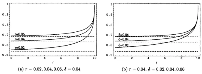
Figures 1(a) and l(b) illustrate

some curves

of thenormalized earlyexercise $boundm\cdot y\xi(t)=$

$\underline{S}(m, T-t)/m$ of theRussian option with finite horizon$T=10$

as

functions of$t\in[0,10]$, where

dashed lines represent the optimal threshold levels $\underline{\xi}_{\infty}$ for the

$a_{\wedge}\backslash \backslash sociated$ perpetual

cases.

The

Table 1: Option values $\tilde{V}(s, m, \tau)/m$ with dividends _{$(r=0.05, \delta=0.03)$} $\ovalbox{\tt\small REJECT} 0.2101.13081.22441260012910\sigma s/.m\tau=1\tau=5\tau.=10\tau.=\infty$

0.9

1.0403 1.1150 11453 11723 0.8 1.0008 1.0378 1.0571

1.0781

0.3 1.0

1.2188

1.4228 1.5273 1.6904 0.9 1.1125 12890 13816 15273 0.8

1.0426

1.1741 1.2517 1.3775 0.4 1.0

1.3130

1.6535 1.8572 2.3065 0.9 1.1940 14950 16771 20803 $\ovalbox{\tt\small REJECT} 0.81.1014$1.35141.50491.8644

Table 2: Option values $\tilde{V}(s, m, \tau)/m$ with no dividends _{$(r=0.05, \delta=0)$}

$\frac{\ovalbox{\tt\small REJECT}\sigma s/.m\tau.=1\tau=5\tau=10\tau=100}{0.210114751.30661.41442.0519}$

0.9 10518 11835 1,2780

₁₈₄₇₈

0.8 1.0061 1.0800 1.1545 1.6468

0.3

1.0

12372

1.5256 1.7391

3.2714

0.9 1.1274 13793 1.5696 29456 0.8 1.0508 1.2472 1.4101 2.6229

0.4

1.0

13329

17766

2.1287

5.0986

0.9

12110

16045

1,9199

₄₅₉₀₃

0.8

11138

14446

1.7202

40855

In these figures, we

can see

that each

curve

ofthe boundaries reaches the value 1 at maturity,

which is consistentwithProposition 3. Thealgorithmworks well

even

near

expiration, depicting

rapidly increasing

curves

as

$tarrow T$

.

Note that Figures l(a) and l(b) provide

a

_numerical check

for the symmetry relation proved in Proposition 5. All of the figuresindicate ageneral property

that the lower the threshold level $\underline{\xi}_{\infty}$, the slower convergence of$\underline{\xi}(\tau)$

as

$\tauarrow\infty$.

5

Conclusion

In thispaper,

we

analyzedtheRussianoption withfinite timehorizonviatheLaplace transform

approachto obtain the LCTs of the option value, the early exercise boundaryand

some

hedging

parameters. all of which can be expressed in terms of the unique real root of a functional

equation.

Our

numerical analysis showed that the accuracyof thisroot plays

an

important role

innumerica.‘ inversionof Laplace transforms with the Gaver-Stehfest methodthat requires

more

than 20-digits precision. Although the Gaver-Stehfest method generates sufficiently accurate

solutions for almost all

cases as

shown in Section 4, the solutions sometimes behave unstably for

the situations where $V(s, m, t)\approx m$, typically _{occurred when} $tarrow T$ or $sarrow\underline{S}(m, t)$

.

Removing

this instability especially around the smooth-pasting point is

an

important problem to be solved

$t$ $t$

(a) $r=0.02,0.04,0.06,$ $\delta=0.04$ (b) _{$r=0.04,$ $\delta=0.02,0.04,0.06$}

Figure 1: Early exercise boundaries $\underline{S}(m, T-t)/m(T=10, \sigma=0.2)$

The Laplace transform approach is

so

general that it could be applied to other

American-stylepath-dependentoptions whose payofffunctions

are

sufficientlysmooth with respect to state

variables, $e.g.$, lookback, barrier, exchange and

so on.

Also, the approach could be extended to

the

cases

that the underlying asset price has jumps and that it is discretely monitored. These

extensions still remain

as

future work.

References

[1] Abate, J. andW. Whitt, “The Fourier-series method for invertingtransforms ofprobability

distri-butions,” Queueing Systems, 10 (1992) 5-88.

[2] Carr, P., “Randomizationand the American put,“ $Re\uparrow yieu$_’

of

Financial Studies, 11 (1998) 597-626.

[3] Duffie, J.D. and J.M. Harrison, ‘Arbitrage pricing ofRussian options and perpetual lookback

op-tions,” Annals

_of

Applied Probability, 3 (1993) $641-()51$

.

[4] Duistermaat, J.J., A.E. Kyprianou and K. van Schaik, “Finite expiry Russian options,” Working

Paper, Utrecht University, 2003.

[5] Ekstr\"om, E., “Russianoptionswithafinite time horizon,” Joumal

_of

Applied Probability,41 (2004)

313-326.

[6] Gaver, D.P., “Observing stochastic processes and approximate transform inversion,” Operations

Research, 14 (1966) 444-459.

[7] Graversen, S.E. and G. Pe\v{s}kir, “On the Russian option: The expected waiting time,” Theory

_of

Probability and theirApplications, 42 (1998) 416-425.

[8] Kimura, T., “Valuing Russian options withfinite time horizon viaLaplace transforms,” Discussion

PaperSeries$A$, No. 2006-171, Graduate School ofEconomicsand BusinessAdministration,Hokkaido

University, 2006.

[9] Kyprianou, A.E. and M.R. Pistorius, “Perpetual options and Canadization through fluctuation

theory,” Annals

_of

Applied Probability, 13 (2003) 1077-1098.

[10] Pedersen, J.L., “Discounted optimal stopping problems for the maximumprocess,” Journal

_of

AP-plied Probability, 37 (2000) 972-983.

[11] Peskir, G., “The Russianoption: Finite horizon,” _{Finance and}Stochastics, 9 (2005) 251-267.

[12] Shepp,L. andA.N. Shiryaev, “TheRussianoptions:Reducedregret” _Annals

_of

_{AppliedProbability,}

3 (1993) 631-640.

[13] Shepp, L. and A.N. Shiryaev, “A newlook at the ‘Russianoption’,” Theory

_of

Probability and their

Applications, 39 (1994) 103-119.

[14] Stehfest, H., “Algorithm 368: Numerical inversion of Laplace transfOrms,” Communications

_of

the

$ACM,$ $13$ (1970) 47-49.