Design and
Dynamics
Copyright © 2013 by JSME
Abstract
This paper presents a control scheme of engine-dynamometer system performing re-al gasoline engine operation in virture-al driver-vehicle-road simulation conditions. The focus is on the transient behavior of the dynamometer speed control during engine-in-the-loop simulation, and a control-oriented model of the dynamometer is constructed. Based on the model, the generalized predictive controller is designed as the external control loop of the existing dynamometer controller to improve the response of the engine-dynamometer system, which reduces the synchronizing speed error between actual engine-dynamometer and the virtual driveline-vehicle model. The performance of the proposed control scheme is verified through comparison experiments includ-ing usinclud-ing the original control without the external control loop and a conventional proportion-differentiation control in the external control loop. The results indicate that the generalized predictive control yields significant improvement in terms of response ability. Finally, a speed following test using the proposed control scheme is conduct-ed, which demonstrates the fast response of the engine-dynamometer system during a transient simulation process.
1. Introduction
Transient control has recently become a major concern in research into the internal com-bustion (IC) engine because of its tremendous influence on engine fuel consumption and emis-sion(1) – (4). To test engine control performance under different operational conditions, engine-dynamometer test benches are widely used in the automotive industry(5), (6). In such systems, the dynamometer is driven to follow a pre-programmed torque or speed profile, which is cal-culated based on the operating mode and route conditions. This test configuration is sufficient to evaluate engine performance under fixed operating profiles. However, it is not sufficient to provide a validity test for the engines operated by any drive style on any given route. The engine-in-the-loop simulation (EILS) system has been the focus of much attention, since the driver-vehicle-route loop is emulated in real time. In the system, the physical engine-dynamometer system is coupled with a virtual vehicle mathematical model. The engine-dynamometer acts as an external load generator and adjusts the engine’s operational state in real time. The key to such a system is to guarantee that the virtual vehicle model is driven by the actual torque generated by the real engine. The control issue of the dynamometer is how to achieve this testing environment by driving the dynamometer, the low-inertia electrical machine.
Nevertheless, in commercial dynamometers, the transient process during speed or torque control could generate an undesired delay in response to the speed track due to induction-to-power delays and dynamometer nonlinearities. Furthermore, there is a coupled relationship between these two control plants (gasoline engine and dynamometer), which influences the engine’s simulation performance in the closed loop control. Therefore, an accurate
mathe-Key words: Engine-in-the-Loop Simulation, Dynamometer Control, Generalized
Predictive Control
Modeling and Control for Engine-in-the-Loop
Simulation System*
Mingxin KANG** and Tielong SHEN**
** Department of Engineering and Applied Sciences,Sophia University, Tokyo, 102-8554, Japan E-mail: [email protected]
*Received 8 Apr., 2013 (No. 13-00011) [DOI: 10.1299/jsdd.7.428]
matical model and a better understanding of the dynamic characteristics of this system are essential to realize precise control.
Many previous studies of the construction and control of EILS have been reported. Bab-bitt et al. proposed the implementation details and test results for a transient engine dy-namometer system(7), (8). In such implementations, the transient engine performance was
cal-ibrated, and the dynamometer worked under the dynamic conditions to emulate the real road load. Hosam et al. reviewed the development and applications of the EILS system and veri-fied the transient emission performance of conventional and hybrid powertrains(9). Bunker et al presented a robust multivariable feedback controller to avoid excessive loop interactions in this closed-loop system. In their research, an engine-dynamometer model used for controller design was developed by spectral estimation techniques and step responses calibration meth-ods(10). Jose designed a decoupled PI action controller for an engine-dynamometer system
based on a transfer function model in order to improve the control response of the test bed(11). The literatures offer some inspirations and insights into methodologies to validate engine tran-sient behavior via integration with a virtual vehicle model and road conditions. Indeed, fast response of the dynamometer control is required in these studies.
This paper mainly focuses on the problem of control design for the dynamometer such that it reduces the synchronized error between the speed response of the vehicle model and the dynamometer under the configuration described. To this end, a simplified kinetic mod-el is presented first, and based on the modmod-el, a generalized predictive control (GPC) scheme is deduced for the dynamometer. The quick response of the dynamometer when the virtual vehicle is driven by the actual engine torque is the aim. Finally, experimental results of the dynamometer control using a conventional proportion-differentiation (PD) feed-forward con-trol and a GPC algorithm were compared to verify the effects of the proposed control scheme, and a speed following test was demonstrated.
2. System Overview and Problem Description
The configuration of the EILS system is shown in Fig.1. The system consists of a real engine, a driver model, a virtual driveline-vehicle dynamics model, and the low inertia elec-trical dynamometer. The driver inputs three signals to the system, the accelerator demand, the gear shift, and the braking demand, while engine electronic control unit (ECU) drives the engine according to the acceleration demand in real-time, and the actual torque generated by the engine forces the mathematical model of the driveline and vehicle to move under the vir-tual environment and load conditions. The purpose of this system is to emulate the situation in which the driver drives the vehicle with a real engine on the road. Thus, the dynamometer must be controlled to guarantee the reality of this situation, especially during the transient process. Vehicle model Dynamometer Controller ECU
M
Accelerator Brake Eng. torque DriverActual vehicle speed
Virtual Driveline Vehicle Model
Engine Dynamometer
Gearshift
In this research, the V6 gasoline engine (Toyota Motor Inc., Japan) is adopted, and the low inertia dynamometer (Horiba Inc., Japan) runs in the speed control mode, with a PID control algorithm in its controller (SPARC). By this inner control loop of SPARC, the dy-namometer forces the engine to work under the virtual road conditions.
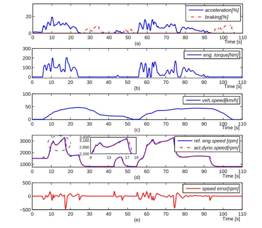
For example, when the road condition is straight and flat, the system is operated ac-cording to driver demands including the acceleration signal and braking command shown in Fig.2(a); the actual engine torque and the vehicle speed are respectively shown in (b) and (c); and the reference engine speed (solid line in (d)) yielded from the mathematical model must be reproduced synchronously by dynamometer speed (dotted and dashed line in (d)). In fact, it is better to have a small synchronizing error between the speed of the virtual model and the actual engine-dynamometer system. However, owing to the signal propagation delay and the causality of the physical system, it is difficult to keep the synchronizing error at ze-ro. In reality, the error between the reference speed command and the actual response of the dynamometer can reach 500r pm, as shown in (e). Besides, the lag time of the dynamome-ter speed control response is about 300ms during the transient test process, which seriously affects the precision of the simulation. Hence, an important challenge here is how to coordi-nate engine-dynamometer transient control responding to the commands from virtual models during the simulation process. Accurate transient control, especially for the dynamometer control system, and fast dynamic response are required to guarantee the safety and control precision of the experiments. The dynamic characteristics of the dynamometer system must be understood before testing.
0 10 20 30 40 50 60 70 80 90 100 110 0 20 (a) 0 10 20 30 40 50 60 70 80 90 100 110 0 100 200 300 (b) 0 10 20 30 40 50 60 70 80 90 100 110 0 50 100 (c) 0 10 20 30 40 50 60 70 80 90 100 110 1000 2000 3000 (d) 0 10 20 30 40 50 60 70 80 90 100 110 −500 0 500 (e) acceleration[%] braking[%] eng. torque[Nm] veh.speed[km/h] ref. eng.speed [rpm] act.dyno.speed[rpm] 9 13 17 19 2,200 2,660 3,160 3,400 speed error[rpm] Time [s] Time [s] Time [s] Time [s] Time [s]
Fig. 2 Example of EILS simulation test.
The problem addressed in this paper is as follows: for any given acceleration signal demanded by the driver, to find a real-time control law to provide the speed command for the dynamometer’s controller, such that the dynamometer speed tracks the speed command of the driveline-vehicle model with satisfactory accuracy and rapidity. In view of the existing control scheme in SPARC is unchangeable and the speed tracking performance is constrained by the
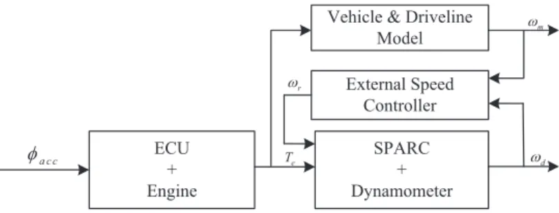
limited gain choice, an external control loop based on the GPC is introduced to improve the speed tracking performance. This achieves accurate simulation for the real engine transient control in the virtual driving conditions. Fig.3 represents the control diagram for speed control of the dynamometer. The reference engine speed command for SPARC given by the driveline-vehicle model will be regarded as the control input of the external control loop, and the actual rotational speed of the dynamometer is the control output.
ECU + Engine SPARC + Dynamometer External Speed Controller Vehicle & Driveline
Model m w r w d w e T a c c f
Fig. 3 Control diagram for speed control of dynamometer.
3. Modeling
3.1. Model StructureIn the system, the engine crankshaft is connected to the dynamometer with a gear box. In order to obtain the kinematical model for the dynamometer, the engine and the dynamometer are simply regarded as two rigid bodies connected with a viscoelastic shaft, as shown in Fig.4, where Jeand Jddenote the inertia coefficient of the engine and the dynamometer, and k and β
are the stiffness and flexibility coefficients of the equivalent shaft, respectively. Terepresents
the engine torque, and Tdis the electromagnetic torque of the dynamometer.
Je
Jd
Engine Dynamometer
Te we wd Td
k b
Fig. 4 Physical model of the engine-dynamometer system.
The dynamic rotation model of the dynamometer can then be described as follows:
Jdω˙d = k ∫
(ωe− ωd)dt+ β(ωe− ωd)− Td− βdωd (1)
where,βd is the rotation damping coefficient, which is determined by the internal physical
structure of the dynamometer.
Given that the electromagnetic torque of the dynamometer is generated by inner-loop control (SPARC controller), the transient dynamics can be simply represented as the first-order system driven by the inner-loop control actuation, i.e., the sum of the proportional and integral of speed tracking error between command speed and the actual speed, since the dynamometer is under PI control based on the speed error. Therefore, the dynamics of the electromagnetic torque can be expressed as follows:
˙
Td = −aTd+ b(ωr− ωd)+ c ∫
(ωr− ωd)dt (2)
where,ωris the command speed of the dynamometer, and a, b, and c are constants that relates
to the response time of the system and the controller performance. 3.2. Parameters Identification
The parameters of the model (1) and (2) can be obtained by applying the well-known identification algorithm for the linear system. To this end, we rewrite the system model as a
linear regression expression by instituting (1) into (2), which yields,
Jdω¨d = k(ωe− ωd)+ β( ˙ωe− ˙ωd)− aTd− b(ωr− ωd)− c(θr− θd)− βdω˙d (3)
where,θdandθrdenote the rotation angle of the dynamometer shaft and the command angle,
respectively. They can be regarded as the integrals of the corresponding speed variables, that is,θd=
∫
ωddt,θr= ∫
ωrdt.
The model is a single-input-single-output (SISO) system, in which input is the speed command and output is the actual speed of the dynamometer. Suppose the sampling period is ∆T, the equation (3) can then be written also in the following discrete-time form with white noise itemε(k):
ωd(k+ 1) = a1ωd(k)+ a2ωd(k− 1) + a3ωe(k)+ a4ωe(k− 1)
+a5ωr(k)+ a6(θr(k)− θd(k))+ a7Td(k)+ ε(k)
(4) where, a1− a7are the parameters to be estimated and they are defined as follows,
a1= 2 +∆T 2 Jd (b− k − β ∆T − βd ∆T), a2= ∆T Jd (β + βd), a3=∆T 2 Jd (k+ β ∆T), a4= −∆T Jd β, a5= −∆T 2 Jd b, a6= −∆T 2 Jd c, a7= −∆T 2 Jd a.
Based on the above discrete model (4), the recursive least square (RLS) method is em-ployed to estimate these unknown parameters. The experimental data used for parameter iden-tification can be collected via the CAN bus, and the sampling period∆T = 0.01s. In order to obtain accurate estimation results, we implemented the only system input, namely the speed control command of the dynamometerωr (shown in Fig.5(a)), to act like a pseudo-random
binary sequence (PRBS), which can sufficiently motivate the system dynamic characteristic. The corresponding dynamometer responses include the actual speedωdand electromagnetic
torque Tdwhich are measured by the sensors inside the dynamometer, as also shown in Fig.5.
0 20 40 60 80 100 800 1000 1200 1400 1600 Speed[rpm] 0 20 40 60 80 100 −50 0 50 100 Time [s] Dyno.torque [Nm] ωr ωd T d (a) (b) Time [s]
Fig. 5 The experimental data used for model identification.
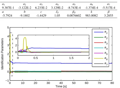
Applying the RLS identification algorithm, the estimated parameters converge to con-stants along with the identification process,which is illustrated in Fig.6. Table 1 lists the identification results of the model parameters.
In order to evaluate the model’s accuracy, another experiment was conducted, and the comparison result between the actual speed and the model’s estimated speed is shown in
Table 1 Identification results of the dynamometer model parameters
a1 a2 a3 a4 a5 a6 a7
9.387E-1 -3.122E-2 6.233E-2 3.129E-2 -8.743E-4 -1.374E-4 -5.517E-4
a b c Jd βd k β -5.7924 -9.1802 -1.4429 1.05 0.0076602 983.0082 3.2855 0 10 20 30 40 50 60 70 80 −1 0 1 2 3 4 5 Time [s] Identification Parameters a 1 a 2 a 3 a 4 a 5 a 6 a 7 0 0.5 1 1.5 2 0 2 4
Fig. 6 The convergence process of identification parameters.
Fig.7. The estimation error between the estimated and the measured results is generally within a margin of 10%. Thus, the proposed model can be deemed acceptable for the controller design. 0 20 40 60 80 100 120 140 160 0 1000 2000 3000 4000 Speed[rpm] Measured Estimated 0 20 40 60 80 100 120 140 160 −12 −8 −4 0 4 8 Time [s] Error [%] Estimation Error 24 26 28 1000 2000 3000
Fig. 7 Comparison between measured and estimated speed.
4. Controller Design
A key specification of EILS is real-time performance, especially in transient operation modes. From the point of controller design for the engine-dynamometer system, the actual speed of the shaft driven by both engine and dynamometer must track the speed of virtual driveline-vehicle with sufficient rapidity and accuracy when the virtual vehicle is driven by the actual engine torque. Thus, for the dynamometer speed control loop that is designed here, the reference signal is provided by the virtual model of the driveline-vehicle. It means that, during real-time simulation, the future values of the reference signal can be calculated in advance based on the mathematical model. This is an incentive to introduce predictive-based control to improve the transient performance. Moreover, GPC control has good robustness,
and is widely applied in engineering practice. In the following,a GPC control scheme is designed.
The objective of the proposed controller is to find a control law for the speed command of the dynamometer such that the actual speed of the dynamometer follows the reference engine speedωmas quickly as possible, where the reference engine speed is the response of the
drive-line and vehicle model driven by engine torque under any given acceleration signal. Therefore, to find a desired controlωr(k) at the step k, the following cost function is introduced:
J= N p ∑ i=1 (ωm(k+ i) − ˆωd(k+ i|k))2+ Nc ∑ j=1 rj∆ωr(k+ j − 1)2 (5)
where, N p and Nc are the predictive horizon and control horizon, respectively. ωm(k+ i)
denotes the response of the driveline and vehicle model at the k+ i(i = 1, 2, · · · , Np) step
and ˆωd(k+ i|k) denotes the model-based i-step ahead prediction from step k, which can be
obtained by repeating the one-step ahead prediction with the system model (1) and (2). The desired control is given by the incremental form,∆ωr(k+ j) = ωr(k+ j) − ωr(k+ j − 1). rjis
the weighting factor of the control variable.
Indeed, solving this optimization problem is a kind of receding horizon optimization process; however, the model-based generalized predictive of ˆωd(k+ i|k) is used in the cost
function, and it can be solved by applying the generalized predictive control (GPC) algorithm presented in [12]. To this end, the system dynamics model mentioned in Section 3 can be represented as following a continuous-time state-space equation:
˙x= 0 1 0 0 −k Jd − β+βd Jd − 1 Jd 0 0 −b −a c 0 −1 0 0 | {z } A x+ 0 0 b 1 |{z} B ωr+ 0 1 Jd 0 0 | {z } Ψ ξ (6)
where, the state variables x= [ θd ωd Td (θr− θd) ]T, speed commandωris the
manip-ulated variable andξ is the external disturbance, which is determined by the engine speed and can be written by the following equation:
ξ = k · θe+ β · ωe.
The dynamometer speed is regarded as the only output of the system; therefore, the output equation can be written as follows:
y =[ 0 1 0 0 ] | {z }
C
x (7)
Thus, the discrete-time state-space equations can be derived from (6) and (7) as follows:
x(k+ 1) = Adx(k)+ Bdωr(k)+ Ψdξ(k)
y(k) = Cdx(k)
(8)
where, Ad, Bd, Cd, andΨd denote the discrete-time forms of the matrices A, B, C, and Ψ in
the continuous-time state-space equations. If∆T is defined as the discrete time, then they are written by following equations:
Ad= eA∆T, Bd= ∫ ∆T 0 e A∆TdtB, Ψ d= ∫ ∆T 0 e A∆TdtΨ, C d= C.
The GPC algorithm usually consists of three basic principles including predictive mod-el, receding optimization and feedback compensation. To solve this problem, the predictive model has to be reformulated first. The augmented predictive model can be written as follows:
xm(k+ 1) = Amxm(k)+ Bm∆ωr(k)+ Ψm∆ξ(k)
y(k) = Cmxm(k)
where, xm(k) = [ x(k)− x(k − 1) y(k) ]T, ∆ωr(k)= ωr(k)− ωr(k− 1), ∆ξ(k) = ξ(k) − ξ(k − 1),
and the incremental matrices Am, Bm,Ψm, Cmcan be described as follows: Am = Ad O4×1 CdAd 1 , Bm = [ Bd CdBd ]T , Ψm= [ Ψd CdΨd ]T , Cm = [ O1×4 1 ].
Based on the above augmented model, the model predictive outputs of future N p steps from the k− th step can be derived by following matrix form:
Y= Fxm(k)+ ΦU + ΛΞ (10)
where,
Y = [ y(k + 1|k) y(k + 2|k) · · · y(k + N p|k) ]T, U= [∆ωr(k) ∆ωr(k+ 1) · · · ∆ωr(k+ Nc − 1)]T,
Ξ = [ ∆ξ(k) ∆ξ(k + 1) · · · ∆ξ(k + Nc − 1) ]T.
Here, the disturbance variables at time (k+ 1),. . ., (k + Nc − 1) are unknown. Suppose that they equals the value at k time. Therefore,Ξ = I∆ξ(k), I is the basic unit vector with
Nc× 1dimensions. The predictive matrices F, Φ, and Λ are written by the following forms: F=[ CmAm CmA2m · · · CmA N p m ]T Φ = CmBm 0 · · · 0 CmAmBm CmBm · · · 0 ... CmA N p m Bm CmA N p−1 m Bm · · · CmA N p−Nc m Bm Λ = CmΨm 0 · · · 0 CmAmΨm CmΨm · · · 0 ... CmA N p m Ψm CmA N p−1 m Ψm · · · CmA N p−Nc m Ψm
The optimal control vector U can be obtained via minimizing the cost function J. From ∂J/∂U = 0, it can be expressed as follows:
U= (ΦTΦ + R)−1ΦT(Rs(k)− Fxm(k)− ΛI∆ξ(k)) (11)
where, the item Rs(k) is the set-point data vector that represents the response of the virtual
driveline and vehicle model in the future N p steps, and R is the weighting coefficient vector that determines the closed-loop control performance. Their expressions are written as follows:
Rs(k)= [ωm(k+ 1) ωm(k+ 2) · · · ωm(k+ N p)]N p×1 R = [r1 r2 · · · rNc]Nc×1
Based on the receding horizon control principle, we take the first element of the control vector at time k as the final incremental control variable, so the control law can be written by
∆ωr(k)= K(ΦTΦ + R)−1ΦT(Rs(k)− Fxm(k)− ΛI∆ξ(k)) (12)
ωr(k) = ωr(k− 1) + ∆ωr(k) (13)
5. Experiments
5.1. Experiment Configuration
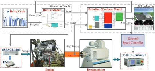
In order to verify the control effects of the proposed GPC control scheme, validation ex-periments have been implemented on the EILS test bench. The configuration of the test bench is shown in Fig.8. In this system, the engine ECU provides a free communication interface and permits engine control to be taken over by the external controller. A programmable con-troller, called dSPACE 1006 processor board, is installed as the top level engine controller to communicate with engine ECU.
0 200 400 600 800 1000 1200 1400 0 10 20 30 40 50 60 70 80 90 100 Time/(s) Vehic le S pe ed/(k m/h ) Vehicle Model
Driveline &Vehicle Model
External Speed Controller
Drive Cycle Driver Model
MicroAutoBox II AVL InMotion
Set-speed Actual speed Eng. Speed Brake Acc. pedal Throttle Engine Dynamometer EMS dSPACE 1006 SPARC Controller (Speed Control Mode)
Torque sensor Eng. Torque
Fig. 8 Physical connection of the EILS test bench.
The virtual system consists of two independent simulation modules. One is the driver-route control model. It can be programmed in the Simulink and compiled as the C code into the MicroAutoBox II (also produced by dSPACE Inc.), which is a programmable controller. Specifically, if given the route information such as drive cycle speed, the driver model will es-timate the operation commands, including acceleration, braking, and gearshift, and then drive the virtual vehicle and perform real engine tracking this reference vehicle speed during the simulation process. Another module is the driveline and vehicle dynamics model. A com-mercialized simulation tool (AVL InMotion) has been adopted here to provide the accurate mathematical vehicle model and real-time motion display. Further, an automatic transmission with five gears has been adopted in the driveline model.
All the necessary data transfer among these different hardwares are achieved via the CAN bus. The engine torque measured by the torque sensor will be delivered to the InMotion and consequently drag the virtual vehicle forward. Meanwhile, the reference engine speed derived from the vehicle speed will feed back to the dynamometer controller in real time. The external speed controller is set up in order to enhance the responsiveness of the speed tracking control of the engine-dynamometer system. The dynamometer then drags the engine to follow the reference engine speed command as quickly as possible. In this closed-loop control system, the minimum lag time is crucial to the engine transient tests, and therefore the proposed GPC scheme will be applied to the external speed control loop of the dynamometer.
5.2. Experimental Results
5.2.1. Case 1: Speed tracking control for dynamometer In this research, we have im-plemented two kinds of experiments to verify the effects of the proposed GPC controller, where we set the predictive horizon N p = 10 and the control horizon Nc = 2. First, the responsiveness of the speed tracking with the external speed controller will be investigated in Case 1. It provides the comparative results for validation of the speed tracking perfor-mance of the dynamometer based on an open-loop control. In this case, the virtual models are
neglected and the engine throttle is kept constant at 8deg. The predefined reference engine speed command will be delivered to the external speed controller of the dynamometer directly. Meanwhile, in order to compare the effects of the proposed GPC controller, a proportional and differential (PD) of the tracking error is also used for the feedback control of the external con-trol loop, and a feed forward action is introduced to obtain quick response. The PD concon-troller is expressed as follows:
ωr(k)= kp· e(k) + kd· (e(k) − e(k − 1)) ·
1
∆T + ωm(k) (14)
where, e(k) = ωm(k)− ωd(k). In this case, the parameters kp = 0.5 and kd = 0.2. Indeed,
GPC is just multi-step ahead predictive control but the PD controller can be regarded as a one-step ahead predictive control due to the function of the differential item. The speed tracking controller is shown diagrammatically in Fig. 9.
ECU + Engine External Speed Controller (GPC/PD) m w d w a c c f r w SPARC + Dynamometer Td Te
Fig. 9 Diagram of the speed tracking controller in Case 1.
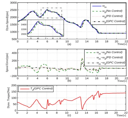
0 2 4 6 8 10 12 14 16 18 20 22 500 1000 1500 2000 2500 3000 Time[s] Dyno.Speed[rpm] 0 2 4 6 8 10 12 14 16 18 20 22 −200 0 200 400 Time[s] Speed Error[rpm] 0 2 4 6 8 10 12 14 16 18 20 22 0 50 100 150 200 Time[s] Dyno. Torque[Nm] ωm ωd(No Control) ωd(PD Control) ωd(GPC Control) ωm−ωd(No Control) ωm−ωd(PD Control) ωm−ωd(GPC Control) Td(GPC Control) 5 6 7 8 9 2000 2200 2400 2600 (c) (b) (a)
Fig. 10 Speed control response test with the dynamic inputs.
Fig.10 shows the comparative test results when giving the system the same dynamic speed command. The reference speed commandωmshown as the solid line in Fig.10(a) should
be followed by the actual speed of the dynamometer as quickly as possible. The dash line represents the actual response of the dynamometer speed control without the external control loop. It is obvious that there is nearly 300ms of lag time for the dynamometer to respond to the given command. However, the lag time can be reduced by the external control loop with the proposed PD controller and GPC controller. The results of the PD control shown as the dotted line can improve the speed response time by about 100− 120ms more than where there
is no control. However, the PD controller more easily induces a large overshoot, especially when the reference speed changes sharply during 12− 14s. However, the result of the GPC controller shows better track performance with lower overshoot compared to the PD control. The synchronizing error between the reference speed command and actual speed is shown in Fig.10(b). It also shows that using the proposed GPC controller yields an overall smaller synchronizing error. Moreover, as one of the main state variables of the system, dynamometer torque changes along with the changes of dynamometer speed, as shown in Fig.10(c).
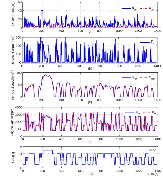
0 200 400 600 800 1000 1200 1400 0 50 100 Vehicle Speed [km/h] v ref vmdl 0 200 400 600 800 1000 1200 1400 0 1000 2000 3000 4000 Engine Speed [rpm] ωm ωd 0 200 400 600 800 1000 1200 1400 0 100 200 300 Engine Torque [Nm] T e 0 200 400 600 800 1000 1200 1400 0 20 40 60 Driver Inputs[%] u thr ubra 0 200 400 600 800 1000 1200 1400 0 2 4 6 Time[s] Gear[1] Gear (a) (b) (c) (d) (e)
Fig. 11 EILS experimental result with driving cycle.
5.2.2. Case 2: EILS closed-loop control The closed-loop EILS experiment integration with the virtual driver-vehicle-route model presented in Fig.8 is implemented in Case 2. The driver model adopts the conventional PID control scheme to control the engine throttle and brake pedal angle to make the vehicle speed tracking the given drive cycle. The driver model is described as follows, um= kp1· ev+ ki1· ∫ evdt+ kd1· dev dt , um∈ [−100, 100] (15)
where, evis the speed error between the vehicle model speedvmdland reference vehicle speed
vre f, ev= vmdl−vre f. The control parameters kp1, ki1, and kd1are set as 10, 5, and 1, respectively.
The driver manipulated variable umcan be specified as the throttle or brake control according
control, an idling buffer area has been set up in this research.
uthr= um, 3≤ um≤ 100 (Throttle Control) uidl = 0, −2 < um< 2 (Idling Control) ubra= −um, −100 ≤ um≤ −2 (Braking Control)
(16)
In order to emulate the operation conditions of the road vehicle, the proposed GPC con-troller is adopted to improve the speed response of the engine-dynamometer system to the virtual model.
Fig.11 shows a typical experimental result with the drive cycle using the proposed EILS test bench. In this experiment, the engine idling speed is set as 800r pm. The engine torque used in the vehicle model is received from the torque sensor in real-time and its low limit is set as 0Nm. During the simulation process, the driver inputs such as throttle and braking signals are shown in Fig.11(a). The real engine torque (shown in (b)) corresponding to the throttle opening drives the virtual vehicle speedvmdltracking with the reference vehicle speed
vre f (solid line in (c)). Meanwhile, the reference engine speedωmis transmitted to the GPC
controller and forces the actual speed of the dynamometerωd to follow it. Owing to the
au-tomatic transmission with five gears adopted in the driveline model of the InMotion software, the gearshift is controlled by the internal control algorithm of InMotion, as shown in Fig.11(e).
800 810 820 830 840 850 860 870 880 890 900 1000 2000 3000 4000 (a) Dyno. Speed [rpm] ωm ωd 800 810 820 830 840 850 860 870 880 890 900 −200 0 200 (b) Speed Error[rpm] ωm−ω d 800 810 820 830 840 850 860 870 880 890 900 0 100 200 300 (c) Engine Torque [Nm] T e 800 810 820 830 840 850 860 870 880 890 900 0 10 20 Time[s] Throttle[%] u thr 835 840 845 850 1000 2000 3000 (d)
Fig. 12 EILS experimental result with driving cycle.
The experimental result represents the feasibility of the proposed EILS system combined with the virtual models of route-driver-driveline-vehicle. Using the external speed controller, the engines can achieve the desired work-points quickly. The local detailed performance of the experiment is extracted and shown in Fig.12. In comparison to the results without the external controller shown in Fig.2, it is obvious that the proposed GPC control scheme reduces the synchronizing error between the reference engine speed calculated by driveline model and the actual speed. It also enhances the responsiveness of the engine-dynamometer system corresponding to the virtual model in the dynamic simulation process. In addition, the test bench provides an emulational operational environment for future research on transient fuel efficiency and emission.
6. Conclusion
A modeling and control method for the engine-dynamometer simulation test bench has been proposed in this paper. In order to precisely conduct engine-in-the-loop tests, the smaller lag time for the engine-dynamometer system responding to the requirement of virtual models is crucial to the precision of the simulation. To this end, an external control loop of the dynamometer was designed, in which the GPC control scheme has been represented to reduce the synchronizing error between the reference engine speed calculated by driveline model and actual speed of the dynamometer. The test results show that the proposed controller enhances the responsiveness of the engine-dynamometer in such a closed-loop control system. Compared with PD feed forward control, the proposed GPC controller obtains better control effects and avoids an unexpected overshoot during the dynamic speed tracking control.
In addition, EILS experiments using GPC control have been introduced in this paper. With the virtual driver-vehicle-route model, the test bench can emulate the engine operation conditions as far as possible. The GPC controller improves the control performance and helps the proposed EILS test bench to achieve accurate simulation tests. It can be further used in the development of fuel efficiency technology and other engine transient control methods in the future.
References
( 1 ) Ericson, C., Westerberg, B., and Egnell, R., Transient Emission Predictions With Quasi Stationary Models, SAE Technical Paper, 2005-01-3852 (2005).
( 2 ) Lee, S., Transient Dynamics and Control of Internal Combustion Engines, Beijing:
Peo-ple’s Transportation Press, Chap. 3 (2001).
( 3 ) Li, S. E. and Peng, H., Strategies to Minimize Fuel Consumption of Passenger Cars during Car-Following Scenarios, 2011 American Control Conference, (2011).
( 4 ) Ross, M., Automobile Fuel Consumption and Emissions: Effects of Vehicle and Driving Characteristics, Annual Review Energy Environment, Vol. 19, (1994), pp.75 - 112. ( 5 ) Nabi, S., Balike, M., Allen, J. and Rzemien, K., An Overview of Hardware-in-the-loop
Testing System at Visteon, SAE Technical Paper, 2004-01-1240 (2004).
( 6 ) Hellstrom, E., Ivarsson, M., Aslund, J. and Nielsen, L., Look-ahead Control for Heavy Trucks to Minimize Trip Time and Fuel Consumption, Control Engineering Practice, Vol. 17, No. 2 (2009), pp. 245 - 254.
( 7 ) Babbitt, G. R., Moskwa, J. J., Implementation Details and Test Results for A Tran-sient Engine Dynamometer and Hardware in The Loop Vehicle Model, Proceedings of
The 1999 IEEE International Symposium on Computer Aided Control System Design,
(1999), pp. 569 - 574.
( 8 ) Babbitt, G. R., Richard, L. R., Bonomo, R. L., and Moskwa, J. J., Design of Integrated Control and Data Acquisition System for A High-bandwidth, Hydrostatic, Transient Engine Dynamometer, Proceedings of the American control conference, Vol. 2 (1997), pp. 1157 - 1161.
( 9 ) Fathy, K. H., Filipi, S. Z., Hagena, J., and Stein, L. J., Review of Hardware-in-the-loop Simulation and Its Prospects in the Automotive Area, Proc. Of SPIE, Modeling and
Simulation for Military Applications, Vol. 6228 (2006).
(10) Bunker, B. J., Franchek, M. A., Thomason, B. E., Robust Multivariable Control of An Engine-dynamometer System, IEEE Transactions on Control Systems Technology, Vol. 5 (1997), pp. 189 - 199.
(11) Lopez, D. J., Espinosa, J. J., and Agudelo, J., Decoupled Control for Internal Combus-tion Engines Research Test Beds, Revista Facultad de Ingenieria University. Antioquia
N., (2011), pp. 23-31.
(12) Wang, L., Model Predictive Control System Design and Implementation using MAT-LAB, published by Springer, (2009).