Spatial and Temporal Modeling of
Heteroscedastic Volatility Behaviors in Social
Science
著者
SATO TAKAKI
学位授与機関
Tohoku University
学位授与番号
11301甲第18407号
Spatial and temporal modeling of heteroscedastic
volatility behaviors in social science
Contents
1 Introduction 3
2 SPATIAL AUTOREGRESSIVE CONDITIONAL
HETEROSKEDAS-TICITY MODELS 12
2.1 Introduction . . . 12
2.2 Spatial Autoregressive Conditional Heteroskedasticity model . . . 14
2.3 Estimation . . . 16
2.3.1 Parameter estimation by the two step procedure . . . 16
2.3.2 Asymptotic results . . . 18
2.4 Empirical Analysis . . . 21
2.4.1 Simulation studies . . . 21
2.4.2 Land price data analysis . . . 22
2.5 Conclusion . . . 23
3 Spatial GARCH Models 31 3.1 Introduction . . . 31
3.2 Spatial GARCH models . . . 33
3.3 Estimation . . . 34
3.3.1 First step estimation . . . 34
3.3.2 Second step estimation . . . 37
3.4 Empirical analysis . . . 38
3.4.1 Simulation studies . . . 38
3.4.2 Land price data analysis . . . 38
3.5 Conclusion . . . 40
4 SARAR-GARCH models 62 4.1 Introduction . . . 62
4.2 Models . . . 64
4.3 Estimation . . . 65
4.4 Real data analysis . . . 66
4.4.1 Japanese market analysis . . . 66
4.4.2 U.S. market analysis . . . 68
Acknowledgments
First, I wish to express the deepest appreciation to my advisor, Professor Ya-sumasa Matsuda, for valuable guidance and encouragement. He is always willing to spend his time with me on research issues and giving suggestions.Without his patience and help, this dissertation would not have been possible.
Second, I am grateful to my dissertation committee members, Professor Nobuhiko Terui and Professor Tsukasa Ishigaki, for their valuable comments and encouragement. They always gave me helpful suggestions and stimulating comments Moreover, I would also like to thank Professor Yoshihiro Yajima and Ryozo Miura for their valuable advice in seminars.
Finally, I have to express my gratitude to my family. They support my study long time.
Chapter 1
Introduction
This thesis is concerned with spatial and spatio-temporal extensions of time series volatility models. Volatility which is a variance and conditional variance in a model is one of the most important concepts in financial econometrics because it is used in widely areas such as risk management, option pricing and portfolio selection. However, volatility has some special features. The daily volatility is not directly observable from market data because we observe only one observation in a trading day. These unobservability makes it difficult to evaluate and forecast volatility. Moreover, financial market data often exhibits volatility clustering (i.e., volatility may be high for certain time periods and low for other periods). This means time-varying volatility is more common than constant volatility. Therefore, accurate modeling of time-varying volatility is important in financial econometrics.
The seminal work of Engle (1982) proposes autoregressive conditional het-eroscedasticity (ARCH) models and the most important extension of the model is generalized ARCH (GARCH) models proposed by Bollerslev (1986). Let rt
be the log return of an asset at time index t. The GARCH (1, 1) model for rt
is defined by rt = σtεt, σt2 = ω + αr 2 t−1+ βσ 2 t−1,
where σt is volatility, εt is random variable belonging to an independent and
identically distributed (i.i.d.) process with mean equal to 0 and variance equal to 1, ω, α and β are parameters. The positivity of σtis ensured by the following
sufficient restrictions: ω > 0, α ≥ 0 and β ≥ 0. The return rt is uncorrelated
but not independent and the dependence of rtcan be described by a linear
com-bination of quadratic function of its lagged values and volatilities. After that, Many extended GARCH models have been proposed. For example, integrated GARCH models ( Engle and Bollerslev (1986)), exponential GARCH models (Nelson (1991)), threshold GARCH models (Glosten, etal (1993)), GARCH in
the mean models, and GJR-GARCH models are proposed.
Univariate volatility models are generalized to multivariate cases in many ways. Financial assets tend to move together over time across both assets, therefore modeling a time-varying covariance matrix is important in may finan-cial applications. Let rt= (r1,t, . . . , rn,t) denote a n-dimensional vector process.
As a natural extension of univariate models, process are defined by,
rt = Σ 1 2 tεt, where Σ 1 2
t is a symmetric matrix square-root of a covariance matrix Σt, such
that Σ12
tΣ
1 2
t = Σt and εt are standardized innovations with mean zero and a
covariance matrix equal to the identity. The curse of dimensionality becomes a major obstacle for generalization because there are n(n+1)2 quantities in a co-variance matrix for a n-dimensional time series. Thus, we attempt to give a conditional covariance matrix some simple structures to reduce the number of parameters. For example, exponentially weighted moving average models, con-stant conditional correlation models (Bollerslev (1990)), BEKK models (Engle and Kroner (1995)), orthogonal GARCH models (Alexander (2001) ), dynamic conditional correlation models (Tse and Tsui (2002)), dynamic orthogonal com-ponent models, and factor GARCH models are proposed.
In this thesis, we apply spatial econometrics ideas to overcome the curse of dimensionality. Spatial econometrics models deal with cross-sectional corre-lation between observations. Therefore, Spatial econometrics models also face the curse of dimensionality because there are n2− n relations that could arise.
The solution to the problem is to impose structure on the spatial dependence relations. We use spatial weight matrices to express the dependence relations between observations and to reduce the number of parameters. Spatial weight matrices are calculated based on distance between observations.
The ideas of spatial econometrics have been applied to volatility models in recent years. Two main objectives of the applications are to reduce parameters in covariance matrices and to extend time series volatility models to spatial models. Caporin and Paruolo (2008) and Borovkova and Lopuhaa (2012) have applied the ideas of spatial econometrics to time series multivariate GARCH models from the former view point. On the other hand, Yan (2007) and Robin-son (2009) have done spatial extensions of stochastic volatility models which are another kind of volatility models and Sato and Matsuda (2017) have extend time series ARCH models to spatial ARCH (S-ARCH) models from both view points.
We propose spatial ARCH (S-ARCH) models, spatial GARCH (S-GARCH) models and spatial autoregressive models with spatial autoregressive error and generalized autoregressive conditional heteroskedasticity processes (SARAR-GARCH) in this thesis. S-ARCH models and S-GARCH models are spatial extensions of ARCH and GARCH models for spatial data. SARAR-GARCH models are a spatio-temporal extension of ARCH models which are defined by spatial weight matrices based on financial distance.
In chapter 2, we propose a spatial extension of time series autoregressive conditional heteroskedastitictiy (ARCH) models to those for areal data. We call the spatially extended ARCH models as spatial ARCH (S-ARCH) models. Suppose we have areal data yi= Y (Ai) for areas Ai, i = 1, . . . , n. The S-ARCH
model is defined by yi = σiεi log σi2 = α + ρ n ∑ j=1 wi,jlog y2j,
where εi is an independent and identically distributed random variable with
mean 0 and variance 1, wi,j ≥ 0 is a spatial weight that quantifies a closeness
form Aito Aj, α and ρ is parameters and ρ is the parameter that describes the
strength of spatial dependence of volatility on surrounding observations. S-ARCH models are re-expressed in the form of spatial autoregressive (SAR) models for logged observations. Substituting log σ2i into the log squred first equation , we have
log y2i = α + ρ n
∑
j=1
wi,jlog yj2+ log ε
2
i,
namely SAR models.
The two parameters are estimated separately by a two step procedure in order to avoid the bias caused by joint estimation by least squares. In the first stage, we estimate only the parameter ρ by the least square method. Since the error term log ε2
i in the model is not a zero-mean process, least square estimator
for α would be biased. In the second stage, we consider the estimation of α. Regarding ε in the error term as independent standard Gaussian variable, we estimate it by maximizing the quasi log-likelihood. Both the estimators for
ρ and α are consistent, while only the estimator for ρ can be proved to be
asymptotically normal.
We carry out simulation studies to evaluate the finite sample properties of the estimators. We consider the S-ARCH model with the following four cases of i.i.d error term εi that follows
• normal distribution,
• Student-t distribution with 3 degrees of freedom, • chi-squared distribution with 1 degrees of freedom, • log-normal distribution.
Notice that all the error distributions were normalized to be mean 0 and variance 1. We find that the estimator for ρ has almost the same means and root of mean squared errors for each of the four error distributions, while the one for
distributions. As the error distribution is more discrepant form Gaussianity, the empirical estimation performance for α is less efficient.
Finally, we apply S-ARCH models to land price data in Tokyo area. Land price data were collected by the Japanese Ministry of Land, Infrastructure ,Transport, and Tourism, which publishes land prices (yen /m2) on many points scattered all over Japan regularly every year. Dividing Tokyo area into 347 dis-crete units consisting of wards, cities and towns, we evaluated the simple average of logged returns included in each unit, resulting in areal data of 347 observa-tions from 2003 till 2014. We find first the significant evidence of S-ARCH effects in each year. Precisely, in the testing problem of H0: ρ = 0, H1: ρ̸= 0,
the t values for ρ are all 5 % significant except for that in 2003. Moreover, we find the so called volatility clustering, namely units with higher spatial volatil-ities are clustered in some specific districts. The identified volatilvolatil-ities in 2010, 2011 and 2012, indicates that spatial volatilities in the coastal areas hit by the Tsunami by the Great East Japan Earthquake in 2011 are higher than those in the other two years. The identified volatilities in 2005-2010, indicates that spa-tial volatilities in central Tokyo grow in 2005-2007, the period of the economics boom, while they are almost extinct in 2008-2010, the period of the recession after Lehman shock. These behaviors of spatial volatilities suggest that spatial volatilities react to economic booms or recessions in the opposite way with time series volatilities, in recalling that typical financial time series volatilities burst in an economic shock while relatively stable in a boom.
In chapter 3, we extends a generalized autoregressive conditional heteroscedas-ticity (GARCH) model for time series to that for spatial data, which we call a spatial GARCH (S-GARCH) model. Suppose we observe spatial data yi on a
spatial area i for i = 1, . . . , n. We shall define S-GARCH models to describe spatial volatilities of yi by yi = √ hiεi, log hi = λ n ∑ j=1 wi,jlog hj+ ρ n ∑ j=1 wijlog y2j+ α + zi′δ,
where √hi is volatility, εi is an independent and identically distributed (i.i.d)
random variable with mean zero and variance 1, zi is (k× 1) non-stochastic
regressors, and wijis a spatial weight that quantifies vicinity from area i to area
j. The matrix Wn, n by n matrix composed of wij, is called a spatial weight
ma-trix. A spatial weight matrix is usually determined by geographical information of spatial data. The first order contiguity weight matrix is a standard choice for it (Sato and Matsuda, 2017). For parameters (λ, ρ, α, δ′)′in this model, λ and ρ describes spatial interactions of volatilities and logged observations. S-GARCH models reduce to S-ARCH models proposed by Sato and Matsuda (2017) when
λ is equal to 0.
Let us re-express S-GARCH models as SARMA models. Denoting log y2=
(log y2
1, . . . , log yn2)′, log h = (log h1, . . . , log hn)′, log ε2= (log ε21, . . . , log ε2n)′, Zn=
(z1, . . . , zn)′, 1n = (1, . . . , 1)′ and In is n× n identity matrix, we have the
equation, we have
log y2 = (λ + ρ)Wnlog y2+ α1n+ Znδ + (In− λWn) log ε2,
which is a SARMA model, one of popular spatial econometrics models. Parameters are estimated by a two step procedure. First step is the esti-mation of (λ, ρ, δ′)′ by QML method. The constant term α shall be estimated separately in the second step, as log ε2 is not zero mean and the estimator for constant term in the first step is biased. In second step, α is estimated by the likelihood different from the one in the first step. Both estimators have consistency and asymptotic normality.
Monte Carlo experiments are carried out to investigate finite sample per-formances of the two stage estimators. we simulate areal data by S-GARCH models, where zi’s are randomly generated form independent normal
distribu-tions and the spatial weights matrix is generated according to Rook contiguity and row normalizing. For the error terms, εi, we consider the three cases: (i)
standard normal distributions, (ii) chi-squared distributions with 3 degrees of freedom and (iii) log normal distributions. The results show the estimators in the firs step, (ˆλ, ˆρ, ˆβ′)′ are nearly unbiased and not sensitive to the choice of the error distributions. On the other hand, the second step estimator, ˆα depends
on the error distribution, ie, is more biased and has larger RMSE for more deviations from Gaussian.
We shall apply S-GARCH models to land price data in Tokyo area in order to demonstrate identification of spatial volatilities. We use prefectural land price research as land price data. The Japanese Ministry of Land, Infrastructure, Transport, and Tourism publishes land prices on sampling points scattered ir-regularly all over Japan in the form of price per m2 in July. We focus on
the land prices over Tokyo area (Tokyo, Kanagawa, Saitama, Chiba, Tochigi, Ibaraki, Gunma) observed yearly form 2009 to 2014. Averaging log returns of land price in municipal units, we obtain land price as yearly observations of areal data. Namely, land price data consists of yearly averaged log returns over 344 discrete areal unit’s from 2010 to 2014. we find that ˆλ, the strength
of interactions among spatial volatilities, are significant after the Great East Japan Earthquake in 2011 until 2013. This suggests that spatial volatility in land prices may have strengthened when the big event occurs. ˆρ, the strength
between spatial volatility and logged squared observations, is as large as the es-timator for that of time series GARCH models. It is seen that ˆλ + ˆρ is estimated
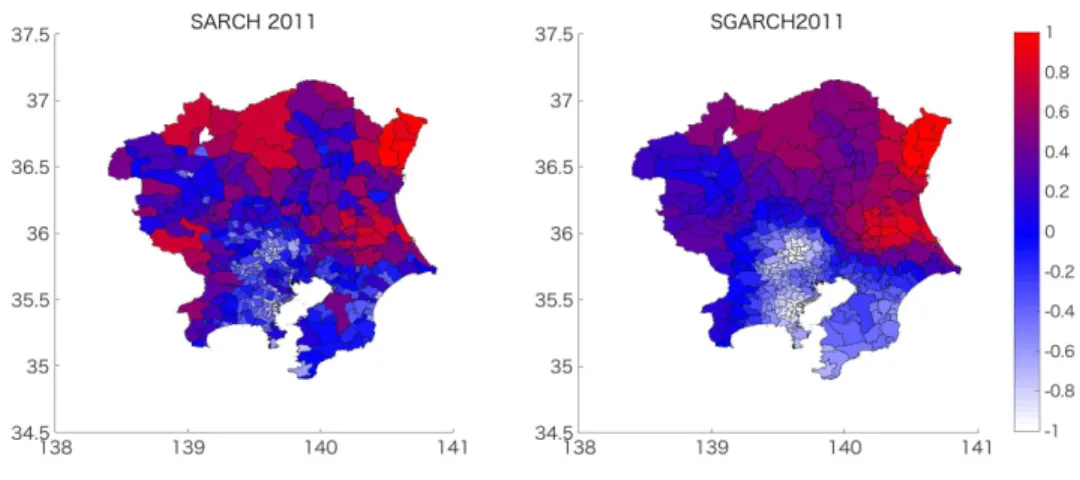
to be close to 1 between 2011 and 2013, which likely causes volatility cluster-ing around coastal areas. We find that volatilities not only at coastal areas hit by the Tsunami but also areas near Fukushima are identified to be high and , which suggests the effects of Fukushima nuclear accidents. Finally in compari-son between identified volatilities by fitting S-ARCH and S-GARCH models, we observe that S-GARCH fits better in terms of AIC with global spillover, which means the identified volatility by S-GARCH models are more highly spatially correlated than those of S-ARCH models.
In chapter 4, we propose spatio-temporal extensions of time series multi-variate volatility models. We call spatiotemporally extended volatility models
as spatial autoregressive models with spatial autoregressive error and general-ized autoregressive conditional heteroskedasticity processes, namely SARAR-GARCH models. Let ri,t be returns of financial instruments. We shall define
SARAR-GARCH models to describe volatilities of return series ri,t by
rt = λW rt+ ut
ut = ρW ut+ εt
εi,t = σi,tfi,t,
fi,t ∼ i.i.d(0, 1),
σi,t2 = ωi+ αiσi,t2−1+ βiε2i,t−1,
where rt = (r1,t, . . . , rn,t), εt = (ε1,t, . . . , εn,t), σi,t is volatility, fi,t is an
in-dependent and identically distributed (i.i.d) random variable with mean zeros and variance 1. The matrix W , n by n matrix, is called a spatial weight matrix and pre-determined before analysis. For parameters (ρ, λ, ωi, αi, βi)′, ρ and λ
describes spatial interactions of return series and ωi, αi and βi are GARCH
pa-rameters. The positivity of σi,t2 is ensured by the following sufficient restrictions:
ωi > 0, αi ≥ 0, βi ≥ 0, and the sum αi+ βi < 1 for stationality. It has been
known that SARMA is guaranteed to exist when|λ| + |ρ| < 1.
A spatial weight matrix is usually determined by geographical information of spatial data and predetermined such as first-order contiguity relation or in-verse distance between observations. However, ri,t is financial data and doesn’t
include geographical information. Therefore, we need to determine financial distances to make a spatial weight matrix. Some author have proposed spatial weight matrix based on financial distance calculated from financial statement data such as dividend yields or market capitalizations. Here, we propose a method to make spatial weight matrices from financial data by stepwise back-ward regression. we apply the multiple linear regression model:
ri,t= δ0+
n
∑
i̸=j
δjrj,t+ zi,t,
where zi,t follows i.i.d normal distribution. Then, we obtain the least square
estimates δj and those t-values. After that we check the minimum t-values
and If the value is smaller than a critical value, for example 1.96, then we remove observations which have minimum t-value. Next, we regress ri,t on n-2
observations and we repeat this procedure until the minimum t-value is grater than the critical value.
We shall propose estimation of the parameters (ρ, λ, βi,j)′in SARAR-GARCH
models. Parameters are estimated by a two step procedure. First step is the estimation of λ and ρ and second step is that of βi,j. Parameter ρ and λ are
estimated in first step. We regard σi,tas constant variance and we apply
quasi-maximum likelihood method with the model. After that we apply GARCH models with residuals derived from first step in second step.
In real data analysis, We apply the SARAR-GARCH model to daily returns of the Nikkei 225 stock price data and S&P 500 stock price data, that is the returns (ri,t) are computed as 100(log Pt−log Pt−1), where Ptis the closing price
and t is the time index referring to trading day t. We compare the in-sample and out-sample performances of SARAR-GARCH models with those of CCC models which is a benchmark. First, we check the in-sample performances based on log-likelihood. The results show the log-likelihood of the CCC model is grater than that of SARAR-GARCH. This means model fitting of the CCC model is better. One reason is that the number of parameters in CCC models is more than five times of those of SARAR-GARCH models. Secondly, we compare out-sample performances. The results shows out-sample performance of SARAR-GARCH models are better. This shows CCC model may be over-fitting and it cause lower forecasting performance. Moreover, we find SARAR-GARCH models work quite well in U.S market analysis. The reason why proposed models work well in U.S market is stock prices in U.S market are more volatile. CCC models assume constant correlation between stock prices so can’t capture dynamic relations, but SARAR-GARCH models can capture dynamic correlation as volatility matrix for the model shown . Therefore, SARAR-GARCH models work well in U.S market.
Bibliography
[1] Alexander, C. (2001). Market models: A guide to financial data analysis. John Wiley & Sons.
[2] Bollerslev, T. (1986). Generalized autoregressive conditional heteroskedas-ticity. Journal of econometrics, 31(3), 307-327.
[3] Bollerslev, T. (1990). Modelling the coherence in short-run nominal ex-change rates: a multivariate generalized ARCH model. The review of eco-nomics and statistics, 498-505.
[4] Borovkova, S. & Lopuhaa, R., (2012). Spatial GARCH: A Spa-tial Approach to Multivariate Volatility Modeling. Available at SSRN: https://ssrn.com/abstract=2176781.
[5] Caporin, M., & Paruolo, P., 2009, Structured multivariate volatility models, Available at SSRN: http://ssrn.com/abstract=1318639.
[6] Engle, R. F. (1982). Autoregressive conditional heteroscedasticity with esti-mates of the variance of United Kingdom inflation. Econometrica: Journal of the Econometric Society, 987-1007.
[7] Engle, R. F., & Bollerslev, T. (1986). Modelling the persistence of condi-tional variances. Econometric reviews, 5(1), 1-50.
[8] Engle, R. F., & Kroner, K. F. (1995). Multivariate simultaneous generalized ARCH. Econometric theory, 11(1), 122-150.
[9] Glosten, L. R., Jagannathan, R., & Runkle, D. E. (1993). On the relation between the expected value and the volatility of the nominal excess return on stocks. The journal of finance, 48(5), 1779-1801.
[10] Nelson, D. B. (1991). Conditional heteroskedasticity in asset returns: A new approach. Econometrica: Journal of the Econometric Society, 347-370. [11] Robinson, P. M. (2009). Large‐ sample inference on spatial dependence.
The Econometrics Journal, 12(s1).
[12] Sato, T. & Matsuda, Y. (2017). Spatial Autoregressive Conditional Het-eroskedasticity Models. J.Japan Statist. Soc., Vol. 47, 2
[13] Tse, Y. K., & Tsui, A. K. C. (2002). A multivariate generalized autoregres-sive conditional heteroscedasticity model with time-varying correlations. Journal of Business & Economic Statistics, 20(3), 351-362.
[14] Yan, J. (2007). Spatial stochastic volatility for lattice data. Journal of agri-cultural, biological, and environmental statistics, 12(1), 25.
Chapter 2
SPATIAL
AUTOREGRESSIVE
CONDITIONAL
HETEROSKEDASTICITY
MODELS
Abstract
This study proposes a spatial extension of time series autoregressive conditional heteroskedasticity (ARCH) models to those for areal data. We call the spatially extended ARCH models as spatial ARCH (S-ARCH) models. S-ARCH models specify conditional variances given surrounding observations, which constitutes a good contrast with time series ARCH models that specify conditional vari-ances given past observations. We estimate the parameters of S-ARCH models by a two-step procedure of least squares and the quasi maximum likelihood estimation, which are validated to be consistent and asymptotically normal. We demonstrate the empirical properties by simulation studies and real data analysis of land price data in Tokyo areas.
2.1
Introduction
This paper aims to extend autoregressive conditional heteroskedasticity (ARCH) models for time series by Engle (1982) and Bollerslev (1986) to those for areal data, which we call spatial ARCH (S-ARCH) models. Areal data is a kind of spatial data that is composed of discrete observations on areal units. See Figure 2.1 for an example of areal data of land prices in Tokyo areas, which are
yearly returns in 2014 on areal units of wards, cities and towns. A S-ARCH model is the one that would describe a conditional variance at an areal unit given data at all other areal units, which we shall call spatial volatility, while a time series ARCH model gives a model to express a conditional variance given past observations, which we call time series volatility. Spatial and time series volatility will be distinguished strictly in this paper. Robinson (2009) has done a spatial extension of stochastic volatility (SV) models for time series (Taylor (2008)). This paper can be regarded as an alternative trial of spatial extensions of time series volatility models in terms of ARCH models.
Figure 2.1: Yearly log returns of the land prices over 347 areal units of wards, cities and towns in Tokyo areas (Tokyo, Kanagawa, Saitama, Chiba, Tochigi, Ibaraki and Gunma prefectures) in 2014.
It is often observed that spatial volatility is not a constant but depends on data at surrounding areal units similarly like time series volatility in financial time series. It is well known that financial time series, even after whitened such as by autoregressive (AR) models, often exhibit substantial dependency in the sense that squared series is serially correlated, which has been accounted for by time series ARCH models (see Tsay (2005)). Hence serial correlations of squared residuals are checked to detect heteroskedasticity of time series volatility.
Let us demonstrate heteroskedasticity of spatial volatility for areal data in the same way as in financial time series case. Land price data in Tokyo areas observed yearly by the Japanese Ministry of Land, Infrastructure ,Transport, and Tourism is employed for the demonstration. Fitting spatial autoregressive (SAR) models (see such as Ord (1975), Kelejian (1999), Lee (2004) and LeSage
and Pace (2009)) to yearly log returns of land price data from 2009 till 2011 to remove linear dependency, we obtain the residuals from the original areal data for each year. Table 2.1 shows Moran’s I’s of the squared residuals as well as those of the residuals, where Moran’s I is an index of spatial correlation that can be regarded as a spatial analogue of lag 1 autocorrelation in time series (Moran (1948, 1950), Anselin (1988)). We find that substantial dependency for the squared residuals still remains, while linear dependency of the residuals is almost null, which suggests heteroskedasticity of spatial volatility exists and that S-ARCH models may work to account for it.
The interesting features of S-ARCH models are summarized as follows. First, the existence condition of S-ARCH models is easily established. Usually it is difficult to check the condition, since S-ARCH models are not Markovian but Markov random fields and so the techniques for Markov models including ARCH models cannot be applied. Secondly, estimators for the parameters in S-ARCH models are well validated to be consistent and asymptotic normally distributed. The paper proceeds as follows. Section 2.2 introduces S-ARCH model. tion 2.3 shows the estimation procedures and their asymptotic properties. Sec-tion 2.4 examines empirical properties of S-ARCH models by applying them to simulated and land price data in Tokyo area. Section 6 discusses some conclud-ing remarks.
2.2
Spatial Autoregressive Conditional
Heteroskedas-ticity model
Suppose we have areal data yi= y(Ai) for areas Ai, i = 1, ..., n. Let us introduce
a spatial autoregressive conditional heteroskedasticity (S-ARCH) model for areal data yi. The S-ARCH model is defined by
yi= σiεi (2.1)
where εis are independent and identically distributed random variables with
mean 0 and variance1, and σi satisfies the following relation:
log σ2i = α + ρ
n
∑
j=1
wijlog yj2, (2.2)
where wij ≥ 0 is a spatial weight that quantifies a closeness from Aito Aj with
wii = 0, and constitutes a spatial weight matrix W = (wij). One popular choice
Table 2.1: Moran’s I’s for the residuals and the squared residuals after fitting SAR models to log returns of land price data in Tokyo areas from 2009 till 2011.
2009 2010 2011 2012 original -0.043 -0.010 -0.036 -0.075 squared 0.152 0.322 0.295 0.246
of the weights wijis the one that takes 1 when Aiand Ajshare the common
bor-der and 0 otherwise. W may not necessarily be dependent on physical distance among areas but on any other abstract closeness such as similarity of financial conditions and so on (Beck et al. (2006)). ρ is the parameter that describes the strength of spatial dependence of volatility on surrounding observations.
S-ARCH models are different from time series ARCH models in the following two points. Firstly, spatial volatility at one areal unit is described by observa-tions at all other units, which is different from time series volatility descripobserva-tions in ARCH models following time flows from past to future. Figure 2.2 is a sim-ple examsim-ple of dependence structures of spatial data demonstrating that spatial volatility at one unit in S-ARCH models can be influenced from observations at all other units. Although time series and spatial volatilities are defined in the different ways, we have found in this paper that they share the similar prop-erties such as significant correlations of squared or absolute processes and the so called volatility clustering which means one large values tend to induce large surrounding and future values in spatial and time series cases, respectively.
Next, the log transformation of σi is used to ensure the existence of areal
data yi. If we defined the spatial volatility similarly with time series ARCH
models by σi2= α + ρ n ∑ j=1 wijyj2,
it would be very difficult to guarantee existence of areal data yi unlike that
for time series ARCH models that can be proved by Markov process theories (Fan and Yao (2003)). The log transformation of σ2
i makes it much easier to
prove the existence in the following way. Substituting log σ2
i in the log squared
equation of (2.1) with (2.2), we have
log y2i = α + ρ n ∑ j=1 wijlog yj2+ log ε 2 i, (2.3)
which is a spatial autoregressive (SAR) model whose existence conditions have been well established. When the matrix I−ρW is non-singular, yiis guaranteed
to exist as
log y2= (I− ρW )−1α1 + (I− ρW )−1log ϵ2,
where log y2= (log y21, . . . , log yn2)′, 1 = (1, . . . , 1)′and log ϵ2= (log ε21, . . . , log ε2n)′.
When W is row normalized, which means the sum of each row of the matrix is normalized to be 1, I− ρW is non-singular if |ρ| < 1. When W is not row normalized, the inverse exists if ρ∈ ( 1
λ(n),
1
λ(1)) where λ(1)<· · · < λ(n)are the ordered eigenvalues of W (Banerjee et al. (2014), Arbia (2014)).
Figure 2.2: Simple example of spatial dependency for 5 areal units. Spatial volatility at one unit can be influenced by observations at all neighboring units simultaneously. Compare time series case when only past observations can in-fluence time series volatility in ARCH models.
2.3
Estimation
We consider the estimation of the two parameters α, ρ in (2.2) and the asymp-totic properties of the estimators. The two parameters will be estimated sep-arately by a two step procedure in order to avoid the bias caused by joint estimation by least squares. We shall show that both the estimators for ρ and α are consistent, while only the estimator for ρ can be proved to be asymptotically normal.
2.3.1
Parameter estimation by the two step procedure
The parameters α, ρ in (2.2) will be estimated separately in the two step proce-dure. Since the error term log ε2
i in the model (2.3) is not a zero-mean process,
joint estimation of α and ρ by the usual least squares (LS) would not work. Specifically the LS estimator for α would be biased because of the non-zero mean error terms. In the first stage we estimate only the parameter ρ by the LS method, while in the second stage we estimate α by the quasi maximum likeli-hood method by regarding εi in the error term as a standard normal variable.
Let us begin from the LS estimation of ρ in the first stage. We slightly modify the original form in (2.3) as
log yi2 = α + E log ε2i + ρ n ∑ j=1 wijlog yj2+ log ε 2 i − E log ε 2 i.
Define three symbols for simplicity by
zi = log y2i,
ϕ = α + E log ε2i,
vi = log ε2i − E log ε
2
Then we have zi= ρ n ∑ j=1 wijzj+ ϕ + vi. (2.4)
Let us estimate ρ in (2.4) by the least squares, which will be obtained by regarding vis as independent Gaussian variables with mean 0. Denoting the
variance of vi as σ2, we have the quasi log-likelihood function of θ = (ϕ, ρ, σ2)′
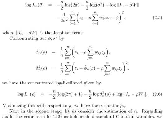
by log Ln(θ) = − n 2 log(2π)− n 2log(σ 2) + log||I n− ρW || − 1 2σ2 n ∑ i=1 ( zi− ρ n ∑ j=1 wijzj− ϕ )2 , (2.5)
where||In− ρW || is the Jacobian term.
Concentrating out ϕ, σ2 by ˆ ϕn(ρ) = 1 n n ∑ i=1 ( zi− ρ n ∑ j=1 wijzj ) , ˆ σ2n(ρ) = 1 n n ∑ i=1 ( zi− ˆϕn(ρ)− ρ n ∑ j=1 wijzj )2 .
we have the concentrated log-likelihood given by
log Ln(ρ) = − n 2(log(2π) + 1)− n 2log ˆσ 2 n(ρ) + log||In− ρW ||. (2.6)
Maximizing this with respect to ρ, we have the estimator ˆρn.
Next in the second stage, let us consider the estimation of α. Regarding
εis in the error term in (2.3) as independent standard Gaussian variables, we
estimate it by maximizing the quasi log-likelihood. If ϵi follows a standard
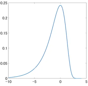
normal distribution, a probability density function of logε2i is easily obtained via change of variables formula as
f (x) = √1 2πexp ( −1 2exp(x) + 1 2x ) . (2.7)
Figure 2.3 shows the probability density function (pdf) of log ϵ2
i.
Then the quasi log-likelihood function of (2.3) based on the density (2.7) is given by log L(α, ρ) = n ∑ i=1 { y2 i exp(α + ρ∑nj=1wijzj) − α + ρ n ∑ j=1 wijzj } −2 log ||In− ρW ||. (2.8)
Figure 2.3: The probability density function of log ε2
i when εifollows a standard
normal distribution.
Differentiating it with respect to α, we have the quasi maximum likelihood estimator given by α = log { 1 n n ∑ i=1 exp ( zi− ρ n ∑ j=1 wijzj )} . (2.9)
Substituting ρ with our proposed estimator ˆρn in the first stage, we propose
ˆ αn= log { 1 n n ∑ i=1 exp ( zi− ˆρn n ∑ j=1 wijzj )} , (2.10) as an estimator for α.
It is possible to estimate ρ and α jointly by maximizing the quasi likelihood in (2.8). The quasi MLEs for them are, however, not validated to be consistent. That is the reason why we propose the two step procedure for the estimation that will be established to be consistent for ˆρn and ˆαn and asymptotically normal
for ˆρn in the next section.
2.3.2
Asymptotic results
This section considers the consistency of ˆρn maximizing (2.6) and ˆαn in (2.10),
and later derives asymptotic normality of ˆρn. Consistency and asymptotic
easily proved independently of ˆρn, while we have not succeeded in deriving the
asymptotic normality.
We will make use of the following set of assumptions. Let ρ0 and α0 be the
true values of ρ and α, respectively.
Assumption 1. {log ε2i}, i=1,...,n, are i.i.d with finite mean and variance. Its
moment E(|logε2|4+γ) for some γ≥ 0 exists.
Assumption 2. The Wn is a row-normalized matrix and uniformly bounded in
column sums, in other words for some real constant c,∑ni=1wij < c for all j.
Assumption 3. The matrix (In− ρ0W ) is nonsingular and (In− ρ0W )−1 is
uniformly bounded in both row and column sums.
Assumption 4. (In − ρW )−1 is uniformly bounded in either row or column
sums, uniformly in ρ in a compact parameter space Θ = [−δ, δ], where δ is smaller than 1. The true ρ0 is in the interior of Θ.
Assumption 5. The limn→∞(Gn1nβ0)′1n/n and limn→∞(Gn1nβ0)′(Gn1nβ0)/n
esist and are nonsingular, where Gn = Wn(In− ρ0Wn)−1 and 1n is a vector
whose elements are all 1.
First, we consider consistency and asymptotic normality of ˆρn.
The covariance matrix of (1/n)∂logLn(θ0)/∂θ is
E ( 1 √ n ∂logLn(θ0) ∂θ · 1 √ n ∂logLn(θ0) ∂θ′ ) =−E ( ∂2logLn(θ0) ∂θ∂θ′ ) + Ωθ,n,
where the average Hessian matrix is
−E ( 1 n ∂2logLn(θ0) ∂θ∂θ′ ) = 1 σ2 0 1 σ2 0n 1′n(Gn1nϕ) 0 ∗ 1 σ2 0n (Gn1nϕ)′(Gn1nϕ) +n1tr((GnG′n)GN) σ12 0n tr(Gn) ∗ ∗ 1 2σ4 0 , and Ωθ,n= 0 µ3 σ4 0n ∑n i=1Gn,ii ∗ 2µ3ϕ σ4 0 ∑n
i=1Gn,iiGi,n+
(µ4−3σ40) σ4 0n ∑n i=1G 2 n,ii ∗ ∗ µ3 2σ6 0 1 2σ6 0n [ϕµ3 ∑n i=1 ∑n j=1Gn,ij+ (µ4− 3σ04)tr(Gn)] (µ4−3σ04) 4σ8 0 , is a symmetric matrix with µj = E(vji), j = 3, 4, being the third, and fourth
moments of vi, where Ginis the ith row of Gn, Gn,ijis the (i,j)th entry of Gn.
Theorem 1. Under Assumptions 1-5, ˆρn converges to ρ0 in probability and
√
n( ˆρn− ρ0)
D
−→ N(0, σρ), σρ is the (2,2) element of matrix Σ−1θ + Σ−1θ ΩθΣ−1θ ,
where Ωθ= limn→∞Ωθ,n and Σθ=− limn→∞E
( 1 n ∂2logLn(θ0) ∂θ∂θ′ ) .
Proof. We show Assumptions of S-ARCH models satisfy the 8 Assumptions of Lee (2004). Assumption 1 of S-ARCH models coincides with Assumption 1 of Lee (2004). Assumption 2 of S-ARCH models suffices Assumptions 2 and 3 of Lee (2004). The first half of Assumption 3 of S-ARCH models is the same as Assumption 4 of Lee (2004). Assumptions 2 and 3 of S-ARCH models suffice the assumption 5 of Lee (2004). The equation (2.4) has an only intercept term as explanatory variables. Therefor, Assumption 6 of Lee (2004) holds. Assumption 4 of S-ARCH models correspond with Assumption 7 of Lee (2004). Assumption 5 of S-ARCH models coincides with Assumption 8 of Lee (2004). Thus, ˆρn is a
consistent and asymptotically normal. Secondly, we consider consistency of ˆαn
Theorem 2. Under Assumptions 1-5, ˆαn converges to α0 in probability.
Proof. The consistency of ˆαn will follow from the convergence in
probabil-ity to zero of ( exp( ˆαn)− exp(α0)).
From (2.10), we have exp( ˆαn) = 1 n n ∑ i=1 exp ( zi− ˆρ n ∑ j=1 wijzj ) . Let logϵ2
i be ζi for simplicity. Thus,
exp ( zi− ˆρ n ∑ j=1 wijzj ) = exp { zi− ρ0 n ∑ j=1 wijzj+ (ρ0− ˆρ) n ∑ j=1 wijzj } , = exp ( zi− ρ0 n ∑ j=1 wijzj ){ exp ( (ρ0− ˆρ) n ∑ j=1 wijzj ) − 1 + 1 } , = exp(α0+ ζi) + exp(α0+ ζi) { exp ( (ρ0− ˆρ) n ∑ j=1 wijzj ) − 1 } . By Theorem 1, (ρ0− ˆρ) ∑n j=1wijzj= (ρ0− ˆρ)(zi− α0− ζi) = op(1)Op(1) = op(1). Since exp((ρ0− ˆρ) ∑n j=1wijzj) p −→ 1, exp((ρ0− ˆρ) ∑n j=1wijzj)−1 p −→ 0.
Moreover, exp(α0+ ζi) = Op(1). Therefore,
exp ( zi− ˆρ n ∑ j=1 wijzj ) = exp(α0+ ζi) + Op(1)op(1), = exp(α0+ ζi) + op(1). Then, exp( ˆαn) = 1 n n ∑ i=1 {exp(α0+ ζi) + op(1)}, = exp(α0) 1 n n ∑ i=1 ϵ2i + op(1).
By the law of large numbers (Brockwell and Davis (2013)),
exp( ˆαn) p
−→ exp(α0) + op(1).
Therefore, exp( ˆαn)− exp(α0)
p
−→ op(1).
2.4
Empirical Analysis
We shall examine the empirical properties of S-ARCH models by applying to simulated and land price data in Tokyo areas. In the simulations we examine finite sample performances of the estimators, while in the real data analysis we check S-ARCH effects in land prices by testing if ρ is positive or zero and evaluate the spatial volatilities identified by S-ARCH models and show them graphically.
2.4.1
Simulation studies
Let us consider the finite sample properties of the estimators ˆρn and ˆαn by
simulated data. The disturbance term in the S-ARCH model is designed as several cases of non-Gaussian as well as Gaussian distributions to see the effects of discrepancy from Gaussianity.
We consider the S-ARCH model in (2.1) and (2.2) with the following four cases of iid error term εi that follows
• normal distribution (norm),
• Student-t distribution with 3 degrees of freedom (t(3)), • chi-squared distribution with 1 degrees of freedom(chi(1)), • log-normal distribution(log-norm).
Notice that all the error distributions were normalized to be mean 0 and variance 1. The spatial volatility was designed by (2.2) with α = 0.3 and ρ = 0.2, where W = (wij), the spatial weight matrix, was the row normalized first-order
contiguity relation for 347 areal units in Tokyo areas whose map is in Figure 1, which will be employed again in the following section of land price data analysis. We have conducted estimation of ρ and α by the two step procedure for 1000 sets of data simulated with each of the four cases of error terms to check the empirical performances of the estimators.
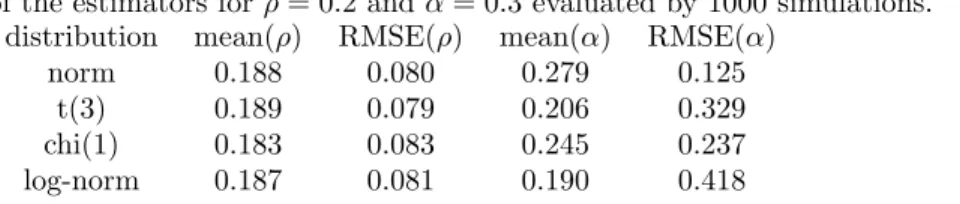
The empirical means and square root of mean squared errors (RMSE) for the two estimators are reported in Table 2.2. We find that the estimator for ρ has almost the same means and RMSEs for each of the four error distributions, while the one for α has empirical means and RMSEs dependent on the error distributions. As the error distribution is more discrepant from Gaussianity, the empirical estimation performance for α is less efficient. It follows that we have
to be careful for a negative bias in the estimation of α when the error term is discrepant from Gaussianity that can cause the identified spatial volatility to be somewhat smaller than the actual ones.
Table 2.2: The empirical means and square root of mean squared errors (RMSE) of the estimators for ρ = 0.2 and α = 0.3 evaluated by 1000 simulations.
distribution mean(ρ) RMSE(ρ) mean(α) RMSE(α) norm 0.188 0.080 0.279 0.125
t(3) 0.189 0.079 0.206 0.329 chi(1) 0.183 0.083 0.245 0.237 log-norm 0.187 0.081 0.190 0.418
2.4.2
Land price data analysis
We apply S-ARCH models in (2.1) to land price data in Tokyo area. We shall examine whether the two properties that are typical in financial time series are detected in land price data. One is S-ARCH effect, which we mean dependen-cies of spatial volatility on surrounding observations, and the other is volatility clustering.
Land price data were collected by the Japanese Ministry of Land, Infrastruc-ture ,Transport, and Tourism, which publishes land prices (yen /m2) on many points scattered all over Japan regularly every year. (http://nlftp.mlit.go.jp/ksj/). Two kinds of land price data are available in the website as prefectural land price research and public land price. Here we chose prefectural land price research published in July every year as data sources, and collected land prices on several thousand points scattered over Tokyo area (Tokyo, Kanagawa, Saitama, Chiba, Tochigi, Ibaraki, Gunma) observed from 2002 till 2014 and transformed them into logged returns from 2003 till 2014. Dividing Tokyo area into 347 discrete units consisting of wards, cities and towns, we evaluated the simple average of logged returns included in each unit, resulting in areal data of 347 observations from 2003 till 2014. Let us denote the logged returns at areal unit i for year t as yit.
<<Table 2.3>>
In prior to S-ARCH model fitting to yit, we apply year by year the following
spatial autoregressive (SAR) model,
yit= β + κ
347
∑
j=1
wijyjt+ uit, uit∼ iid(0, τ2), (2.11)
to remove spatial correlations. Here, W = (wij), the spatial weight matrix,
is given by the row normalized first-order contiguity relation that takes 1 only when sharing common boarders for 347 areal units in Figure 2.1. Table 2.3 shows
the estimated values of ˆβ, ˆκ and ˆτ2 in the SAR model in each year. We find the substantial correlations caused by ˆκ ranging around 0.8-0.9, which means
strong similarities of land price returns among neighboring areal units.
<<Table 2.4>>
<<From Figure 2.4 to Figure 2.6>>
To the residual ˆ uit= yit− ˆβ − κ 347 ∑ j=1 wijyjt,
which are obtained after fitting the SAR models, we applied the S-ARCH model in (2.3) year by year, where the same spatial weight matrix as that in the SAR model was employed. Table 2.4 shows the estimated values of ρ and α in each year, where the standard errors of ˆρn, which are derived in Theorem 2 by
replacing the population moments with the corresponding sample ones, are also shown in parenthesis. Figures 2.4-2.6 express the spatial volatility evaluated by
ˆ σi2= exp ˆα + ˆρ∑347 j=1 wijlog(ˆu2j) .
We find first from Table 2.4 the significant evidence of S-ARCH effects in each year. Precisely, in the testing problem of H0 : ρ = 0, H1 : ρ ̸= 0, the t
values for ρ are all 5 % significant except for that in 2003. From Figures 2.4-2.5, we find the so called volatility clustering, namely units with higher spatial volatilities are clustered in some specific districts. Figure 2.4, which shows the identified volatilities in 2010, 2011 and 2012, indicates that spatial volatilities in the coastal areas hit by the Tsunami by the Great East Japan Earthquake in 2011 are higher than those in the other two years. Figures 2.5, which shows the identified volatilities in 2005-2010, indicates that spatial volatilities in central Tokyo grow in 2005-2007, the period of the economics boom, while they are almost extinct in 2008-2010, the period of the recession after Lehman shock. These behaviors of spatial volatilities suggest that spatial volatilities react to economic booms or recessions in the opposite way with time series volatilities, in recalling that typical financial time series volatilities burst in an economic shock while relatively stable in a boom.
2.5
Conclusion
We have proposed a spatial autoregressive conditional heteroskedasticity (S-ARCH) model to evaluate spatial volatility. Describing logged volatility with linear combinations of logged observations in S-ARCH models, we have estab-lished the conditions that guarantee the existence of S-ARCH models. Re-expressing S-ARCH models in the form of spatial autoregressive (SAR) models
for logged observations, we propose the two step procedure to estimate the pa-rameters ρ and α in S-ARCH models. Both the two estimators are validated to be consistent asymptotically, while the estimator for ρ is shown to be asymptot-ically normal as well as consistent. Finite sample performances of the procedure are reasonably good from our simulation studies. In the land price data analysis, we detect S-ARCH effects by testing if ρ is positive and find volatility clustering that reacts to economic shock oppositely with that in financial time series .
We complete the paper by describing possible extensions for future research. In the empirical analysis of land prices, we used the first-order contiguity rela-tions as the spatial weight matrix. As (Beck et al. (2006)) shows, spatial dis-tances that differ from geographic disdis-tances can be more interesting to improve our volatility analysis using S-ARCH models. We evaluated spatial volatility for fixed t only year by year. Spatio-temporal extensions of S-ARCH models would make it possible to analyze volatility jointly in space and time and to provide a more detailed analysis of volatility structures.
Bibliography
[1] Anselin, L. (1988). Spatial Econometrics : Methods and Models, Kluwer Academic Publishers, The Netherlands.
[2] Arbia, G. (2014). A Primer for Spatial Econometrics: with Applications in
R, Springer-Verlag, New York.
[3] Banerjee, S., Carlin, B. P. and Gelfand, A. E. (2014). Hierarchical Modeling
and Analysis for Spatial Data, Chapman & Hall/CRC, Boca Raton.
[4] Beck, N., Gledrrsch, K. S., and Beardsley, K. (2006). Space is more thn geography: Using spatial econometrics in the study of political economy,
International Studies Quarterly., 50(1), 27–44.
[5] Bollerslev, T. (1986). Generalized autoregressive conditional heteroskedas-ticity, J. Econ., 31(3), 307–327
[6] Brockwell, P. J., and Davis, R. A. (2013). Time Series: Theory and
Meth-ods, Springer-Verlag, New York.
[7] Engle, R. F. (1982). Autoregressive conditional heteroscedasticity with es-timates of the variance of United Kingdom inflation, Econometrica, 50, 987–1007.
[8] Fan, J., and Yao, Q. (2003). Nonlinear Time Series, Springer-Verlag, New York.
[9] Kelejian, H. H., & Prucha, I. R. (1999). A generalized moments estimator for the autoregressive parameter in a spatial model, International economic
review , 40(2), 509–533.
[10] Lee, L. F. (2004). Asymptotic distributions of quasi‐ maximum likelihood estimators for spatial autoregressive models, Econometrica, 72(6), 1899– 1925.
[11] LeSage, JP., & Pace, R. K. (2009). Introduction to Spatial Econometrics, CRC Press, Boca Raton.
[12] Moran, P. A. (1948). The interpretation of statistical maps, J. R. Stat. Soc.
[13] Moran, P. A. (1950). A test for the serial independence of residuals,
Biometrika, 37(1-2), 178–181.
[14] Ord, K. (1975). Estimation methods for models of spatial interaction. J.
Am. Statist. Assoc., 70(349), 120–126.
[15] Robinson, P. M. (2009). Large‐ sample inference on spatial dependence,
Econom. J., 12(s1), S68-S82.
[16] Taylor, S. J. (2008). Modelling Financial Time Series, world scientific, Singapore.
[17] Tsay, R. S. (2005). Analysis of Financial Time Series, John Wiley & Sons, Hoboke.
T able 2.3: Estimated v alues and their standard errors for κ, β and τ 2 in the spatial autoregressiv e (SAR) mo del in (2.11) applied to log returns of land price data in T oky o y ear b y y ear in 2003-2014. . 2003 2004 2005 2006 2007 2008 2009 2010 2011 2012 2013 2014 κ 0.865 0.836 0.805 0.830 0.933 0.848 0.880 0.700 0.820 0.831 0.880 0.892 (0.031) (0.033) (0.033) (0.028) (0.016) (0.027) (0.024) (0.046) (0.030) (0.028) (0.023) (0.021) β -0.408 -0.423 -0.359 -0.096 0.037 -0.002 -0.270 -0.452 -0.250 -0.174 -0.083 -0.037 (0.104) (0.094) (0.071) (0.050) (0.046) (0.031) (0.065) (0.076) (0.048) (0.037) (0.026) (0.022) τ 2 0.668 0.607 0.524 0.781 0.689 0.333 0.380 0.276 0.236 0.215 0.179 0.156 (0.136) (0.144) (0.151) (0.097) (0.110) (0.228) (0.202) (0.282) (0.322) (0.352) (0.424) (0.486)
T able 2.4: Estimated v alues, their standard errors and t-v alues of ρ and estimated v alues of α in the S-AR CH mo del in ref2.1 applied to the residuals b y fitting SAR mo dels to log returns of land price data y ear b y y ear. 2003 2004 2005 2006 2007 2008 2009 2010 2011 2012 2013 2014 ρ 0.082 0.189 0.227 0.274 0.392 0.192 0.357 0.228 0.211 0.255 0.344 0.277 se( ρ ) 0.083 0.079 0.077 0.075 0.069 0.079 0.071 0.077 0.078 0.076 0.072 0.075 t( ρ ) 0.987 2.398 2.925 3.633 5.672 2.435 5.018 2.954 2.708 3.350 4.788 3.687 α -0.254 -0.137 -0.227 0.192 0.348 -0.608 -0.132 -0.781 -0.929 -0.885 -0.719 -0.939
Figure 2.4: The identified volatilities in 2010-2012. Notice that the great earth quake occurred and the coastal areas were hit by great Tsunami in 2011.
Figure 2.5: The identified volatilities in 2005-2010. Notice that Lehman shock occurred in 2008 when economic boom completed and serious recession began.
Chapter 3
Spatial GARCH Models
Abstract
This paper extends a generalized autoregressive conditional heteroscedasticity (GARCH) model for time series to that for spatial data, which we call a spatial GARCH (S-GARCH) model. S-GARCH models specify conditional variances of spatial observations given those on surrounding areas, which is a good contrast with time series GARCH models that specify those given past observations. We employ a two step procedure to estimate parameters in S-GARCH models after transforming them into special kinds of spatial econometrics models, ie spatial autoregressive moving-average (SARMA) models, and derive consistency and asymptotic normality of the estimators. Simulation studies and applications to land price data in Tokyo areas are conducted to demonstrate empirical proper-ties of S-GARCH models.
3.1
Introduction
Volatility models for financial time series have been developing with their fruit-ful applications in financial industries. The seminal work by Engle (1982) in-troduces a autoregressive conditional heteroscedasticity (ARCH) model, while Bollerslev (1986) extends it to a generalized ARCH (GARCH) model. These models have been widely used to identify volatilities that play significant roles in pricing options or measuring values at risk of financial positions in risk manage-ment. Subsequently, multivariate extensions have been conducted by Bollerslev et al (1988), Bollerslev (1990) and Engle and Kroner (1995) for modeling dy-namic relationships of volatilities among multiple asset returns. A major chal-lenge of multivariate volatility modeling is to overcome curse of dimensionality;
n(n+1)/2 components in volatility matrices for n-dimensional asset return series
require complicated modeling and estimation procedures when n is large. One solution for the problem is to consider simpler structures of volatility matrices to reduce parameter dimensions.
Applications of spatial econometrics to volatility modeling have begun in re-cent years in order to extend volatility models for financial time series to those for spatial areal data. Spatial volatility is defined as a conditional variance on an area given observations over all other areas, which is a spatial analogy of time series volatility. Spatial weight matrix plays a key role to construct mod-els for spatial volatilities. See Caporin and Paruolo (2008) and Borovkova and Lopuhaa (2012) for multivariate extensions of GARCH models by spatial econo-metrics methodology, Yan (2007) and Robinson (2009) for spatial extensions of stochastic volatility (SV) models, and Sato and Matsuda (2017) for those of ARCH models, which we named spatial ARCH (S-ARCH) models.
The aim of the paper is to conduct a spatial extension of GARCH models, which we call spatial generalized ARCH (S-GARCH) models. S-GARCH mod-els are regarded as extensions of S-ARCH modmod-els of Sato and Matsuda (2017) in similar ways of extensions from time series ARCH to GARCH models. S-GARCH models are characterized by the following two features. First, spatial volatility at one area depends on volatilities as well as observations over sur-rounding neighbors, which is an extension of S-ARCH models whose volatility depends only on surrounding observations (Sato and Matsuda, 2017). Secondly, S-GARCH models can be transformed into a kind of spatial econometrics mod-els called spatial autoregressive moving average (SARMA) modmod-els by which S-GARCH models are guaranteed to exist and several popular techniques in spatial econometrics literatures are to be applied to estimation and kriging for spatial volatilities.
For estimating parameters in S-GARCH models, we employ quasi-maximum likelihood (QML) estimation and prove consistency and asymptotic normality for QMLE. There are two kinds of popular estimation in spatial econometrics lit-eratures. First one is estimation by moment methods. See Kelejian and Robin-son (1993) and Kelejian and Prucha (1997, 1998) for two stage least squares, and Lee (2007) for the generalized method of moments (GMM) for spatial autore-gressive (SAR) models and spatial autoreautore-gressive models with autoreautore-gressive disturbances (SARAR). In addition, see Dogan and Taspinar (2013) for GMM estimation for spatial autoregressive models with moving average disturbances (SARMA). The other one is estimation by QML methods. See Lee (2004), Yu et al (2008) and Su and Yang (2015) for QML estimation for SAR models and spatial dynamic panel (SDP) models and Yang (2018) for M-estimator based on QML for SDP models. This paper employs the latter approach for estima-tion, namely applies QML method to SARMA models to estimate parameters in S-GARCH models, as S-GARCH models can be transformed into SARMA models.
This paper proceeds as follows. Section 3.2 introduces S-GARCH models and discusses their characteristics. Section 3.3 proposes two step estimation proce-dure for S-GARCH model and derives asymptotic properties of the estimators. Section 3.4 demonstrates applications of S-GARCH models to simulated and real spatial data of land price data in Tokyo areas. Section 3.5 concludes the paper. All the proofs for the asymptotic properties in Section 3.3 are collected in the Appendix.
3.2
Spatial GARCH models
Suppose we observe spatial data yion a spatial area i for i = 1, . . . , n. We shall
define S-GARCH models to describe spatial volatilities of yi by
yi = √ hiεi, log hi = λ n ∑ j=1 wijlog hj+ ρ n ∑ j=1 wijlog y2j+ α + z′iδ, (3.1)
where √hi is volatility, εi is an independent and identically distributed (i.i.d)
random variable with mean zero and variance 1, zi is (k× 1) non-stochastic
regressors, and wijis a spatial weight that quantifies vicinity from area i to area
j. The matrix Wn, n by n matrix composed of wij, is called a spatial weight
ma-trix. A spatial weight matrix is usually determined by geographical information of spatial data. The first order contiguity weight matrix is a standard choice for it (Sato and Matsuda, 2017). For parameters (λ, ρ, α, δ′)′in this model, λ and ρ describes spatial interactions of volatilities and logged observations. S-GARCH models reduce to S-ARCH models proposed by Sato and Matsuda (2017) when
λ is equal to 0.
S-GARCH models describe logged spatial volatilities by linear combinations of spatial lagged values of logged volatilities and observations, which is a spa-tial analogy of time series GARCH models. Although spaspa-tial and time series volatilities are completely different, it will be shown in Section 4 that they share some common features such as volatility clustering, namely a large change at one area causes large changes at surrounding areas.
We must notify here that S-GARCH models describe logged volatilities, while time series GARCH models describe volatilities without log transforma-tion. The logged volatility makes it possible to re-express S-GARCH models as SARMA models. The SARMA expression results in providing two useful key features for GARCH mdoels. First one is that existence conditions for S-GARCH models are easily checked by regarding them as SARMA models. Time series GARCH models are guaranteed to exist by regarding them as Markov pro-cesses (Fan and Yao, 2003). The same technique of Markov propro-cesses cannot be applied to S-GARCH models as there are no orders for spatial data unlike time series. The other one is that several popular tools such developed in spa-tial econometrics literatures can be employed for S-GARCH modeling. Quasi maximum likelihood (QML) method, one of critical estimation tools in spatial econometrics, shall be applied to estimate parameters in S-GARCH models in Section 3.
Let us re-express S-GARCH models as SARMA models. Denoting log y2=
(log y2
1, . . . , log yn2)′, log h = (log h1, . . . , log hn)′, log ε2= (log ε21, . . . , log ε2n)′, Zn=
(z1, . . . , zn)′, 1n = (1, . . . , 1)′and Inis n×n identity matrix, we have the vector
log y2 = log h + log ε2 (3.2) log h = λWnlog h + ρWnlog y2+ α1n+ Znδ, (3.3)
where Wn is the spatial weight matrix composed of wij. It is easy to see from
(3.3) that,
log h = (In− λWn)−1(ρWnlog y2+ α1n+ Znδ),
Substituting the equation into (3.2), we obtain
log y2 = (In− λWn)−1(ρWnlog y2+ α1n+ Znδ) + log ε2,
Multiplying In− λWn from the left, we have
(In− λWn) log y2 = ρWnlog y2+ α1n+ Znδ + (In− λWn) log ε2,
which reduces to
log y2 = (λ + ρ)Wnlog y2+ α1n+ Znδ + (In− λWn) log ε2, (3.4)
which is a SARMA model, one of popular spatial econometrics models (Dogan and Taspinar (2013)). It has been known that SARMA is guaranteed to exist when|λ| + |ρ| < 1 , and hence S-GARCH momdels are guaranteed exist under the same condition as a result.
3.3
Estimation
We shall propose estimation of the parameters (λ, ρ, α, δ′)′ in S-GARCH mod-els and derive the asymptotic properties of the estimators. Parameters are estimated by a two step procedure. First step is the estimation of (λ, ρ, δ′)′ by QML method. The constant term α shall be estimated separately in the second step, as log ε2in (3.4) is not zero mean. and the estimator for constant term in the first step is biased. In second step, α is estimated by the likelihood different from the one in the first step.
3.3.1
First step estimation
Parameters λ, ρ and δ are estimated in first step by the QML estimation method. To apply QML method, we need to demean the error term. Observing in (3.4) that
α1n+ (In− λWn) log ε2 = α1n+ (In− λWn){log ε2− E(log ε21)1n+ E(log ε21)1n},
we see the intercept term has the bias by (1−λ)E(log ε21). Denoting Yn= log y2,
Xn= [1n, Z], Vn={log ε2− E(log ε12)1n} and β = ({α + (1 − λ)E(log ε21)}, δ′)′,
we have the following modified representation,
Yn= λWnYn+ ρWnYn+ Xnβ + (In− λWn)Vn, (3.5)
where Vn is the zero mean processes.
Now, let us consider the QML estimation of (3.5). Regarding v′is as indepen-dent Gaussian variables with mean zero and variance σ2, the likelihood function
of (3.5) is log Ln(ψ) =− n 2 log(2πσ 2)−Vn′(θ, β)Vn(θ, β) 2σ2 − log |Rn(λ)| + log |Sn(θ)|, (3.6) where θ = (λ, ρ)′, ψ = (β′, σ2, θ′)′, Rn(λ) = In−λWn, Rn= In−λ0Wn, Sn(θ) = In−λWn−ρWn, Sn = In−λ0Wn−ρ0Wnand Vn(θ, β) = R−1n (λ)[Sn(θ)Yn−Xnβ].
The QML estimator is the extreme estimator derived form the maximization of (3.6).
It is convenient to work with the concentrated likelihood by concentrating
β and σ2 out for computation and asymptotic analysis on the estimator. From
the first order condition of (3.6), the concentrated QML estimators of β and σ2
is ˆ βn(θ) = (Xn′R′−1n (λ)R−1n Xn)−1Xn′R′−1n (λ)R−1n (λ)Sn(θ)Yn, ˆ σ2n(θ) = ˆ Vn′(θ) ˆVn(θ) n ,
where ˆVn(θ) = R−1n (λ)[Sn(θ)Yn− Xnβˆn(θ)]. The concentrated likelihood
func-tion of θ is log Ln(θ) = − n 2(log(2π) + 1)− n 2 log ˆσ 2 n(θ)− log |Rn(λ)| + log |Sn(θ)(3.7)|.
The QML estimator ˆθn maximizes the concentrated likelihood function (3.7)
and the QML estimators of β and σ2 are ˆβ
n(ˆθn) and ˆσn2(ˆθn), respectively.
For our analysis of the asymptotic properties of first step estimators, we need the following assumptions:
Assumption 6. The disturbances{vi}, i = 1, . . . n are i.i.d. across i with zero
mean, variance σ2
0 and E|vi|4+η <∞ for some η > 0.
Assumption 7. The elements wn,ij of Wn are nonnegative and row normalized
and the column sums of Wn are uniformly bounded.
Assumption 8. The space Θ is compact, and the true parameter θ0 lies in its
interior.
Assumption 9. The matrix Sn, Sn(θ), Rn, and Rn(λ) are uniformly bounded