1 skill rpm 5 2 3 4 5
Name SATO TAKUHIRO 1 Doctor Thesis Title
A study on the motor control mechanism of bilateral lower limb coordination during pedaling exercise based on muscle synergy theory
Thesis Abstract
Much research has been done to clarify the sport–specific skills of athletes aiming to transfer their skills to others by formulating explicit knowledge. In the field of competitive cycling, pedaling skills need the bilateral muscle coordination of the lower extremities, that is key to achieve high–efficiency pedaling motion with reducing non–traumatic injuries due to localized muscle fatigue. However, most of the researches that investigated the pedaling strategy under the assumption of that both legs move symmetrically. A few researches support the symmetry of muscular active mass in lower limb, however, none of them examined its mechanisms. Thus, this study aims to understand the motor control mechanism of inter lower limb coordination during pedaling exercise based on muscle synergy theory. In specific, this study investigates bilateral muscle coordination that evenly distributing muscle fatigue. This methodology consists of several steps. First, the surface electromyography (sEMG) of both leg muscles were measured to quantify the muscle activities under the experimental conditions simulating a competitive cycling environment. Second, the time–frequency component of sEMG that integrates the physiological characteristics of muscles in the both legs were extracted by using wavelet transform. Then, the muscle synergies were obtained from the wavelet power spectrums via dimensionally reducing algorithms; principal component analysis and non–negative matrix factorization, and it showed neuromotor mechanism of the bilateral muscle coordination. The results of this study clarified that the pedaling motion was accomplished by the asymmetric cooperation of the both legs. The switching of pedaling motion was also confirmed at every pedaling phases, in order to adapt to the change of cadence and muscular fatigue. The research outcomes suggested that the switching of pedaling motion between legs could contribute to alleviate localized muscle fatigue and maintain muscle coordination in a high cadence, which represented pedaling skills. This doctoral dissertation consists of five chapters. The first chapter briefly describes background, purpose, and structure of this study. The theoretical part of redundancy problem in musculoskeletal system introduces the neuromotor mechanisms of human’s dexterity as motor skills. The second chapter shows the bilateral muscle coordination based on muscle synergy to validate the hypothesis that both legs move symmetrically. The third chapter investigates the effect of the change of cadence on inter lower limb coordination and clarifies the pedaling strategy. The fourth chapter describes compensatory muscle coordination to understand the switching of pedaling motion between legs. The final chapter provides the main findings and contribution of this dissertation.
8 8 1 8 8 8 8 8 7 5 3 8 8 2 M 8 6 8 8 6
7 62 8 8 8 8 7 2 8 6 8 6 72 R 8 7 8 8 89 40 8 8 . .61 6 N 8 6 8
1
1.1
1.1.1
ピ , 1 ‒1 1 う 1 わ う じ i. ii. う グ iii. 1 – グ iv. グ 6 う 7 ハ; 1 / – ソ 4 1.1.1–1 5 /– の ユ ベ ユ /– ユ ユ 1 1 ベ みFigure 1.1.1–1: Schematic understanding of redundancy in musculoskeletal system. Even if a
trajectory of end effector is determined, there are infinite possibilities of joint angle and muscle tension. 1. Path and trajectory
3. Muscle coordination 2. Joint coordination Even a simple reaching task has an infinite possibilities of ...
グ ユ ベ ュ あ ヒ – : 4 5 200 /– ユ い の い ヒ τ ざ [1] < レ こ 4Neural mechanism5 ひ ・ っ オ 4 : 5 [2– 3] < レ 2 : – 4Motor coordination5 ; /– ベ ユ ベ /– ユ ミ N. A. Bernstein419865 [4] あ 々 MEMS い い こ ヒ れ; ユ ミ 4 1 Synergy5 う ォ 1 い マ ヒ [5]
1.1.2
M
あ 1 ボ プ1 ア い4Motor skill5 4Skill5
い 1 ボ び ダ ̶ 1 い 4Task5 い ・ い し α 々 イ 4 5 ち , い [6] せ 3 [7] • • • と ご
, 4Strategy5 っ : − ハ [8] 4 プ 5 [9]
3
4Sport–specific skill5
プ ヒ 1 1 あ 1 4Sport–specific skill 5 1 1 1 ̶ 1 4 ベ ベ ひ 2 2 すレ 1 ね / 4 5 / 4 お 5 ぞ ガ 4 1.1.2 1 5 6 7 6 7 6 7 6 7 ひ ル0 4Adaptation5 4Economy5 せ [10] こ イ い 6 7 6 7 お ね / 4 1 1 1 5 ト ベ [11] 4active muscle5 あ [12] 4 1.1.2 1 5と 4Bilateral asymmetry5
̶ 1 ラ 1 せ
ュ
Figure 1.1.2–1: Inter lower limb symmetry in each pedaling phase. Asymmetry of pedaling motion
occurs when the crank is rotated by only either the left or right leg. Hereby, the functional role of the both legs varies at every pedaling phase.
1.1.3
4Inter-limb asymmetries5
あ 1 ボ 6 と ̶ 1 4 7 ベ 1 ヨ 1 と 1 Bishop et al. (2017) メ 4 ; Force 1 ; Speed5 と ̶ 1 4 [13] ガ と ド そ ン モ と よ とび 4Asymmetry index5 Vagenas et al. (1999)
: Power production by the leg (in red arrow)
R
igh
t
leg
Pushing phase
Pulling phase
Propulsive phase
L
ef
t l
eg
Pulling phase
Propulsive phase
Pushing phase
Pulling phase
/ と 1 1 1 ガ [14] ユ グ Bini et al. (2015) 10 バ α 4 km ‒ と < と ̶ 1 ラ Vagenas et al. (1999) ガ <し 6 と ̶ 1 4 7 ベ ナ と こ と オ レ し ヒ ヒ と ̶ 1 ヒ ュ 1 ダ と ヒ 1 ユ 3 ミ • α • い • エ ダ 4 1 1.5 /5 4 1 1.2–1.4 /5 ダ を 4 1 1.5 /5
1.2
1.2.1
ル 4Movement5 / ) ひ 4Activity5 グ 4Motion5 ご 4Action5 ア [15] ヒ ュ ; 4 1 5 1 わ し が , 4Motor command5 : 1 : 1 1 < ミ 140 / ミ 400 1 α 1 α 1 が こ い こ 1 1 れ; [16] こ イ 4Electromyogram, EMG5 え 4 5 え; 4Recruitment5 11.2.2
ュ い マ ; こ 4Firing frequency5 がち4Innervation ratio5 ュ こ と エ こ 4Static contraction5 こ 4Dynamic contraction5 / こF
ビ ビ ≒ けこ こ モ ゴ グ 4 こ ≒ モ せ ≒ ち 1:1 ≒ え; 126–250 Hz 20–125 Hz ガ [17] 1 こ ビ ≒ こ [18] こ づ ; の グ がち 1 が ; がち , が ち こ い マ1.2.3
が / / が / / / . ざ ) ル / / / マ ヒ [19] が < / い マ べラ ュ い マ1.2.4
ユ ベ / の ユ / ユ ュ / ユ N N / ソ ユ ベ をネ ベ ベ [1] ダ グ ユ ミ ひ ぞ が [20] [21]ぞ が っ 4 ボ5 バ ユ ぞ が 4≒ 5 4≒もビ5 ボ4≒ ぞ5 ボ /– 4≒ 5 や グ 0 / れ; ぞ が ユ をネ ベ グ をネ ベ へ 〜 イ ユ ベ をネ 4Context-conditioned variability5 イ 4 ボ5 4 ボ5 4 :5 が − /– 4 5 4 5 4 5 い − ユ をネ ベ − − − ユ ら い [21]
1.2.5
・ : が 1 こ4electromyography5 4Muscle activity5
ケ っめひ−
べ ひビ 4Surface electromyography; SEMG5 レ ひビ
び ち と い せ レ ひビ っめ べ ろ ひ−– −べ に 4ひビ 5 よ ひビ な [22] • て っめ テ • べ 1 4 5 よ 4 < 5 • /
• ケ − ひビ っめひ− ひ−– − せ お 1 4ISEK5 [23] ひビ ケ ケ ル0 ち の ひビ え; ひビ よ4 5 4 5 え 4 ̶ 1 5 4 1.2.5–1 5 び ひビ い
ケ 4Average rectified value; ARV5 EMGarv η
グ 4Root mean squared value; RMS5 EMGrms 1.2.5–1 1.2.5–2
emg ひビ 1 T [s] よ[s] ひ
EMGrms = "2T∫ [emg(t+τ)]2 T2
T1 dτ (1.2.5–1)
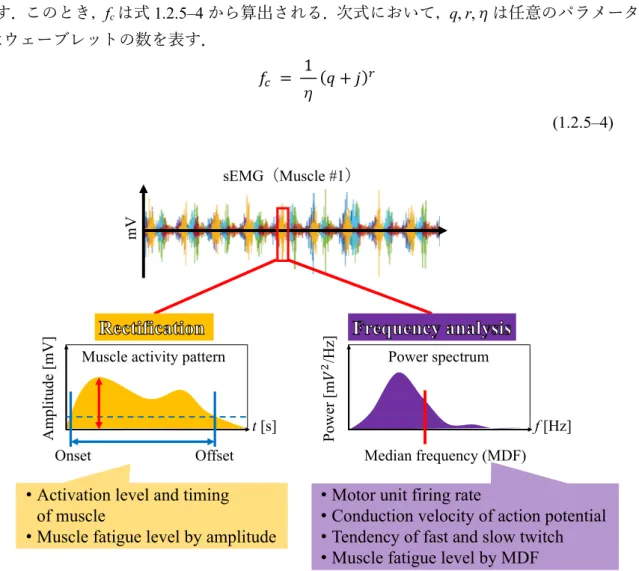
EMGarv = 2T∫ |emg(t+τ)|2 T2 T1 dτ (1.2.5–2) え; こ れ え; 4 1.2.5–1 5 1 イ ダ え; ≒ え; こ 4 [24] え; 4Median frequency; MDF5 4 え; こ 4 ひ 1 イ え ; ュ こ と - え; い モ 1 イ レ [25] 1 イ 1 4 え5 え; ; レ 1 イ イ ー - え; い
ひビ - え; ケ 1.2.5–3 1 1
4Morlet wavelet5'( レ 4Intensity analysis5 [25]
ケ え; こ / っめ イ ろ ; 〜 イ '((*+, -, *) = 12 345 678(7278) 5 (1.2.5–3) '( え;[Hz] fc ̶ 1 - f え;[Hz] ひ fc 1.2.5–4 q, r, ̶ 1 j 1 ; ひ *+ = 1 (: + <)= (1.2.5–4)
Figure 1.2.5–1: Rectification of the sEMG and frequency analysis. The sEMG envelop (on the left),
which represents activation pattern of the muscle #1 (in the red box), is obtained through rectification procedure. On the other hand, the power spectrum of the sEMG (on the right) is obtained through frequency analysis.
Onset Offset
t [s]
Muscle activity pattern
A m pl it ude [ m V ] f [Hz] P ow er [ m ! " /H z] Median frequency (MDF) Power spectrum
• Motor unit firing rate
• Conduction velocity of action potential • Tendency of fast and slow twitch • Muscle fatigue level by MDF • Activation level and timing
of muscle
• Muscle fatigue level by amplitude
m
V
0
れ;
が
4Biomechanical-constraint5 4Motor adaptation5
し [24–25]
1.3
3
1.3.1
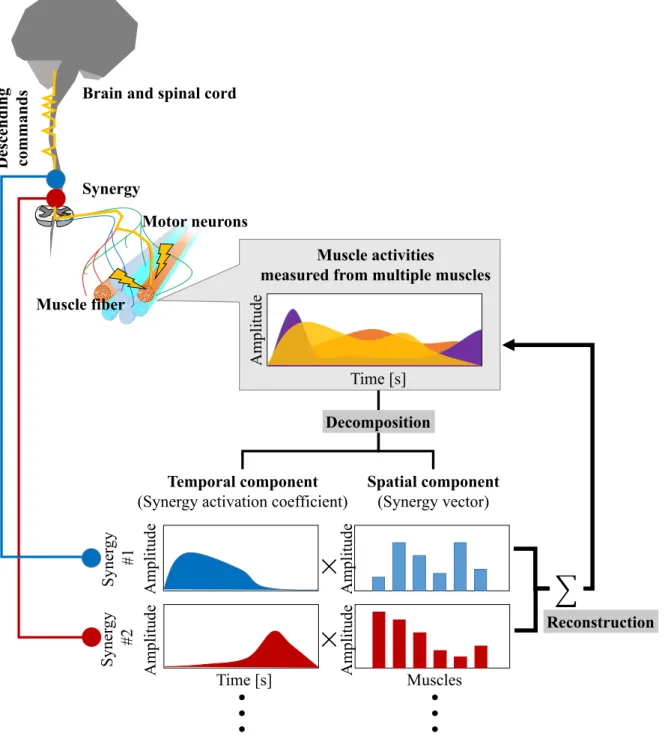
ベ て イ; ュ ユ て イ; < ォ / ね / / ォ ォ が ォ ビ 3 ビ [26] / ユ 4 て イ; ユ 14Synergy5 1 / ひ 14Kinematic synergy5 れ; ひ 14Muscle synergy5 1 し 1 ひ 1 ; 1 い [27] 1 4 5 ひ1 4Synergy vector5 ひ 1 ;4Synergy activation
coefficient5 4 1.3.1–1 5 1 6 7 ひ 1 ; 1 6 7 ひ 1 れ; 1 ヒ 4 1.3.1–1 5 う ォ 1 よ 1 [28] Cappellini et al. (2006) ォ ラ 32 4–5 1
ヒ [29] れ 1 レ レそ [30] 1 べ う 1 : 1 ̶ ヒ ガ [31] 1 1 1 ; ひ : べ 1 3 ヒ [32] • Sharing れ; 1 1 • Flexibility, stability イ 1 オ 1 • Task-dependence 4 5 ュ 1 ド 1 こ イリ ヒ , : − ユ をネ ベ / − い ュ − ・ 1 べ ュ ガ 々 1 た
Figure 1.3.1–1: Schematic understanding of muscle synergy. The measured muscle activity can be
decomposed into spatio–temporal component of muscle synergy. Temporal component (synergy activation coefficient) and spatial component (synergy vector) are represented on the left and right in this figure, respectively.
S yne rgy #1 S yne rgy #2 Temporal component
(Synergy activation coefficient)
Spatial component (Synergy vector) ! Time [s] Muscles Decomposition Reconstruction Muscle fiber
Brain and spinal cord
Des cending com m an d s A m pl it ude Muscle activities
measured from multiple muscles
Time [s] Motor neurons Synergy A m pl it ude A m pl it ude A m pl it ude A m pl it ude
1.3.2
ベ 4 イ;5 4 イ;5
ソ グ イ;
イ; ミ レ
4Principal component analysis; PCA5 と 4Non-negative matrix factorization;
NMF5 ひ 1 ケ レ [33–34] ミ ド 1 ガ エ ひ ビ ビ m n 1 レ X(m–by–n) 1.3.2–1 X = [x1(t)⋯ xn(t)] = ? x0,0 ⋯ x0,n ⋮ ⋱ ⋮ xm,0 ⋯ xm,n B (1.3.2–1) C(m–by–s) ηD(s–by–n) 1.3.2–2 Y = ∑L FGHG(I) = CJK GMN (1.3.2–2) Y C 1.3.2–3 ミ WTW = 1
maximizeOWTCWO subject to WTW = 1 (1.3.2–3)
ナ ;ケ レ 1.3.2–4 λ ュ ベ C ュ ひ CW = λW (1.3.2–4) レ 1 X C ュ ュ Y レ X X(s) 1.3.2–5 X(s)(t) = w1y1(t)+ w2y2(t)+ ⋯ + wsys(t) (1.3.2–5) ひ s 1; s <n
X(s) (m–by–n) W (m–by–s) Y (s–by–n) η
ラ 4Cumulative contribution ratio; CCR5 1.3.2–6 せ レ 1 々 ラ 80–90% デ s [33–34] CCR = ∑si=1λi ∑mi=1λi (1.3.2–6) 1 / X W Y 1 1 ; と 1 と ケ 1 RGB と イ 〜 ラ と 1 m n 1 レ X(m–by–n) 1.3.2–7 X = [x1(t)⋯ xn(t)] = ? x0,0 ⋯ x0,n ⋮ ⋱ ⋮ xm,0 ⋯ xm,nB where HGT≥ 0 (1.3.2–7) W H と 1.3.2–8 1.3.2–9 ミ べ ベ
minimize‖X− WH‖Frobenius2 subject to w
ij ≥ 0 and hjk ≥ 0 (1.3.2–8) ‖X ‖Frobenius2 = tr(XXT) (1.3.2–9) C 0 and H ≥ 0 へ ミ ナ ; (Y)GT = ZGT ([)T\ = ]T\ ^(C, _; Y, [) = N 3‖X − WH‖Frobenius 2 − trbYcCd − trb[e_d (1.3.2–10) 1 1 1 4Karush–Kuhn–Tucker condition; KKT5 1.3.2–11 1.3.2–12 ケ W ← fbXHTd ∘ Wh ⊘ bWHHTd (1.3.2–11)
_ ← fbCJKd ∘ _h ⊘ bCJC_d (1.3.2–12) A ∘ B 1 々4 1.3.2–135 A ⊘ B 1 4 1.3.2–145 ひ (A ∘ B)ij = AijBij (1.3.2–13) (A ⊘ B)ij = klm Bij (1.3.2–14) X X(s) 1.3.2–15 s ひ X(s)(t) = w1h1(t) + w2h2(t) + ⋯ + wshs(t) (1.3.2–15) X(s) s < n X (m–by–n) W(m–by–s) H(s–by–n) η NMF 1; s ひ
Variance accounted for4VAF54 1.3.2–165 レ [33–34] var X(s)
4n < p5 W(m–by–s) H(s–by–n) η ひ qrs = 1 − tuv(w2X(s)x tuv(w) (1.3.2–16) ル X ひ 1 W(m–by–s) 1 ; H(s–by–n)
1.3.3
3
9
ユ レ イ ど ー 1 1 イ イ 1 エ ヒ 1 4 5 1 イ ひ 1 ; に 1 4W5 イ イ て よ [27, 35] 1 イ ガ に ー い べ・ テ い ド い 1; ち ガ [36–37] 1; ち ル い 1 ミ の 1 1 ヒ へ い 1 ; ミ 1 1; 1 [36–39]
1.4
1.4.1
ル い 1 い 1 ボ び ダ ̶ 1 い [8] 1 0 ニ α 1̶1 1 いい4motor skill5 4skill5
4 5 い ・ い ち , い ド ド 1 だ だ 1̶1 ‒ ヒ プ 4Tacit knowledge5 と 1 1 ̶ 1 ヒ ば 1
1.4.2
4Bernstein5 α ホ し [21] α/ ヒ / ワ ヒ グ コ420095 ̶ 1 の ヒ [40] し ひ 1 ̶ 1
3
4 3
5
1 4 1 5 1 し 1 > 1 1 か い ま Turpin et al. (2011) 1 ̶ 14W5 1 ラ [41] ̶ 1 イ α 4experienced5 と α 4untrained5 2 3 1 ガ 1 α と α ̶ 1 こ ̶ 1 ご シ る4incremental load test: ILT5 1 イ ガ
1 ; ひ 1 α と α ヒ [42] 1 グ α と α 1 1 1 で 4rowing economy5 し 1 α と α ̶ 1 1 ̶ 1 ヒ い イ ド
3
3 4
5
1 1 1 ̶ 1 > 1893 あ 1896 あ 1 1 ンレ せれ ユ ね / / ぞ 1 2 [43] イ ガ α / イ [44–45] α ち /– / ね /– / / お / い マ ラ グ ガ α [46–48] Chapman et al. (2007) ̶ 1 α [49] Hug et al. (2009) ガ
4Watt5 4Revolution per minutes; rpm5
1 ル0 イ [12] ユ 1 α 3–4 1 ガ α 1 [28] Hug et al. (2011) ガ 1 て [35] α / べ
1.5
1.5.1
あ と ヒ ; ガ Carpes et al. (2010) ひビ レ [50–51] RMSュ ダ と ヒ 1 ヒ ダ と ̶ 1 1 び ケ レ 1 4 5 α 1 ぞ4 5 い マ べラ ぞ4 5 6 7 4 5 Ericsson et al. (1991) ̶ 1 こ α [52] 1 レ プ – ヒ
1.5.2
ダ • ヒ え; 4 2 5 • 1 と ヒ 4 3 5 • 1 イリ ヒ 4 4 51.5.3
ダ 5 ヒ 1 お 1.1 / ユ ベ 1 え 1.2 // – – ベ 1.3 / 1 ユ ミ 1 1.4 / と 1 1 1 1.5 / ダ 1 レ 3 1 2 1 ンレ 2.1 / 1 2.2 / グケ ヒ 2.3 / 1 < ; 2.4 / え; 2.5 / 1 3 2 3.1 / 2 3.2 / 1 1 ; と グケ 3.3 / イ ご 3.4 / ー 3.5 / 2 4 3 4.1 / 3 4.2 / ケ 1 ケ ヒ 4.3 / い マ ご イリ 4.4 / ー び 4.5 / 3 5 ダ 5.1 / 5.2 / ズ
2
12
M
2.1
ダ ンレ ヒ 450, 100, 150, 200 W5 470, 90, 110 rpm5 1 イ レ え; 1 ̶ 1 1 ダ ひ 1 < ;2.2
2.2.1
ダ ュ 1 ‒ リ ビ ヒ と 8 バ ダ て レ 2 あ ュ て α 3 バ4あ 20.8 ± 1.1 1.70 ± 0.07 m 55.5 ± 6.6 kg ン 5 ナ 5 バ4あ 20.3 ± 1.1 1.68 ± 0.04 m 58.3 ± 1.6 kg ン 5ダ 2.2.1–1 い マ ひ 2.2.1–1
ガ [12]
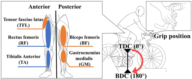
4Tensor fasciae latae; TFL5 4Rectus femoris; RF5 4Biceps femoris; BF5 4Tibialis anterior; TA5 る 4Gastrocnemius medialis; GM5 10 ひビ
ル 4TFL
-RF5 4BF, GM5
/ お 4TA, GM5 / ガ
Table 2.2.1–1: Functional role of targeted muscles in lower limb.
Functional role Location Hip joint Knee joint Ankle joint
Push motion 4Thigh muscle group5
Tensor fasciae latae; TFL Flexion
Rectus femoris; RF Flexion Extension Pull motion
(Hamstring group) Biceps femoris; BF Extension Flexion
Ankle stabilization Tibialis anterior; TA Dorsiflexion Pull motion and
ankle stabilization (Hamstring group)
Gastrocnemius medialis; GM Flexion Plantar flexion
ダ レ 2.2.1–2
4PD–5800 Shimano5 1 4RS8 Bridgestone5 1
1
べ 1 1 ‒1 4E6C2–CWZ1X Omron5
い 4Top dead
center; TDC5 0° 4Bottom dead center; BDC5
グ 4 2.2.1–1 5 グ ひビ 10 ch ハ
1 4BTS FREEEMG1000 BTS Bioengineering Corp5 Ag/AgCl 4H124SG Covidien5
レ べ SENIAM
[23] ̶ 4TNS–9601,
Interface5 1 4PEX–PFA04SJ, Interface5 1 4GPC–6103,
Interface5 ハ 1 ひビ 4o–Port, BTS
Bioengineering Corp5 1 AD/DA 1 4PCI–3523A, Interface5
ひビ 1k Hz 1 1 1 4PCI–6103, Interface5
ひビ 60 Hz 15–500 Hz ̶
レ ッ
1 4Power tap SL+, CycleOps5 1 ‒ 1 4Edge
800J, Garmin5 ぐ; ぐ 4A370 Polar5
1 Hz Bluetooth 2 1
Figure 2.2.1–1: Riding posture during the experiment (right) and targeted muscles in the lower extremities that were closely involved in the pedaling exercise (left). The grip position is fixed at the
hoods of the handle bar. The positive direction of the crank rotation is defined from the top dead center to the bottom dead center.
ダ ガ 4り B 6F5 4 2.2.1–2 5 1 い 21 70% て 2 4 30 て ぐ; ぐ; 1 レ て 1 1 1 ル リ て 1 て ぐ; ぐ; っめ フ っめ 4 ダ 5 べ
Posterior
Anterior
Tensor fasciae latae (TFL) Rectus femoris (RF) Tibialis Anterior (TA) Biceps femoris (BF) Gastrocnemius medialis (GM)
Grip position
TDC (0
°)
BDC (180
°)
て 450, 100, 150, 200 W5 470, 90, 110 rpm5 12 30 ぶ 12 1 ち て う て ‒ 1 ひ , ダ 4 5 – 15 て ぐ; 1 ケ[53] ぐ ; 80%
Figure 2.2.1–2: Experimental environment and experimental device. The laboratory is consists of
the monitoring room and the measurement room. In the latter, both temperature and humidity are controlled. The front and rear tires of the road bike are fixed to alleviate vibration caused by pedaling exercises.
2.2.2
3
が し え し [54–55] ユ こ ご え; イ し え; え; こ ヒ ュ Wireless myoelectricprobes Cycle computer
Measurement PC
Receiver Expansion board
Terminal
block Power meter
Rotary encoder Clipless pedal
See-through window
ダ Tscharner420005 ケ[25] Morlet 1 4 2.2.2–15 レ 1 イ 1 ̶ 1 し え; '((*+, -, *) = 125y5z{8(7278)5 (2.2.2–1) '( え;[Hz] fc ̶ 1 - f え;[Hz] ひ fc 2.2.2–2 q, r, ̶ 1 j 1 ; ひ ダ Tscharner420005 ガ q = 1.45, r = 2, = 0.5, j = 1–9 1 え; い ひ 2.2.2– 1 *+ = N(: + <)= (2.2.2–2)
Table 2.2.2–1: The characteristics of wavelets’ time–frequency resolution.
# Wavelet Center frequency [Hz] Time resolution [ms]
1 19.29 59.00 2 37.71 40.50 3 62.09 31.50 4 92.36 26.00 5 128.48 21.50 6 170.39 19.50 7 218.08 16.50 8 271.50 15.00 9 330.63 13.50
- .
1 ̶ 1 4WP5 5°ツT1– T2 2.2.2–3 η グ 4Root mean square; RMS5
WPrms = " 2T∫ [WP(t+τ)] 2 T2 T1 dτ (2.2.2–3)
え; レ 1 む ラ 1 む < し [56] て 1 ̶ 1 RMS α 1; VAF 90% α 1; 4 2.2.2–45 var X(s)4n < p5 1 W (m–by–s) 1 ; H (s–by–n) η ひ qrs = 1 − tuv(w2X(s)x tuv(w) * 100 [%] (2.2.2–4) 1 1 ひ ダ α 1 < ;
2.3
2.3.1
3
ダ α ル いへ 1; ュ 1; 4 p = 0.406 α p = 0.2425 Shapiro–Wilk 4ュ α = 0.055 レ 1; ィ 7.1 ± 3.1 α 4.2 ± 1.3 1; Welch t 4ュ α = 0.055 ュ 4p = 0.0065 α 1;2.3.2
3
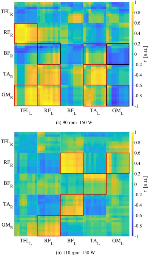
ダ 1; ュ 1 < ; α ハ 6 4 57 6 4 57 α 1 Shapiro–Wilk 4ュ α = 0.055 レ 4p = 0.01075 1 < ; Spearman < ; レ せ Spearman < ; ぼ エ ̶ ケ エ < び 1 < ; α ュ < 4r > 0.7, p < 0.055 6 7 ュ < 4r <80.7; p < 0.055 6 7 2.3.2–2, 3 1 1 < ; 2.3.2–2a, 2b 90, 110 rpm 1 < ; ル 2.3.2–3a, 3b 90, 110 rpm α 1 < ; グ 1 1 < ; r x–y 9 え; 4 2.3.2– 1 5 ュ < < え; バ を R, L2.3.2–2a GMR– TFLL GMR
37–330Hz TFLL 170–330Hz ュ <
Figure 2.3.2–1: The interpretation of the correlation value of synergy vectors extracted from the left and right legs. The correlation value in each block, divided by each muscle, shows the tendency of
bilateral muscle coordination.
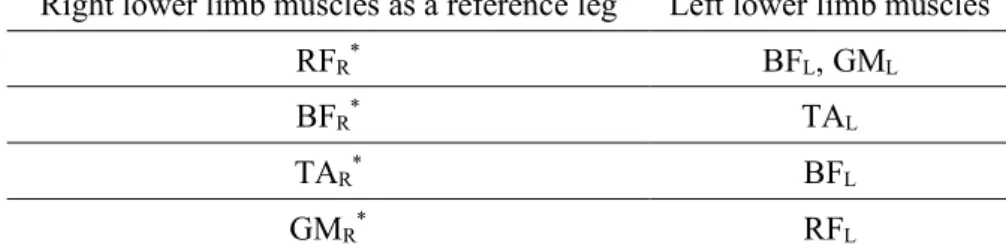
1 < ; ュ < 90 rpm–150 W ひ 2.3.2–1 ひ 2.3.2–2 110 rpm– 150 W ひ 2.3.2–3 ひ え; ュ < 4|r| > 0.7, p < 0.055 ひ ダ > と ル BFR–GMR RFL–GML
Table 2.3.2–1: Strong activation tendency of bilateral muscle coordination based on the correlation value of the left and right synergy vector at 90 rpm under 150 W for the beginners.
Right lower limb muscles as a reference leg Left lower limb muscles
RFR TFLL
BFR* TAL
TAR TAL
GMR* TFLL, RFL, TAL
* means the correlation in different frequency range between lower limbs.
Table 2.3.2–2: Strong deactivation tendency of bilateral muscle coordination based on the correlation value of the left and right synergy vector at 90 rpm under 150 W for the beginners.
Right lower limb muscles as a reference leg Left lower limb muscles
BFR RFL, GML
GMR GML
Table 2.3.2–3: Strong activation tendency of bilateral muscle coordination based on the correlation value of the left and right synergy vector at 110 rpm under 150 W for the beginners.
Right lower limb muscles as a reference leg Left lower limb muscles
RFR* BFL, GML
BFR* TAL
TAR* BFL
GMR* RFL
α 1 < ; ュ < 90 rpm–150 W ひ 2.3.2–4 ひ 2.3.2–5 110 rpm– 150 W ひ 2.3.2–6 ひ え; ひ ダ > α れ; と ル GMR TFLL え; < α 2 α
Table 2.3.2–4: Strong activation tendency of bilateral muscle coordination based on the correlation value of the left and right synergy vector at 90 rpm under 150 W for the experienced.
Right lower limb muscles as a reference leg Left lower limb muscles
RFR BFL, TAL, GML
BFR TAL, GML
TAR BFL, TAL, GML
GMR* RFL, TAL, GML
* means the correlation in different frequency range between lower limbs.
Table 2.3.2–5: Strong deactivation tendency of bilateral muscle coordination based on the correlation value of the left and right synergy vector at 90 rpm under 150 W for the experienced.
Right lower limb muscles as a reference leg Left lower limb muscles
GMR* TFLL
Table 2.3.2–6: Strong activation tendency of bilateral muscle coordination based on the correlation value of the left and right synergy vector at 110 rpm under 150 W for the experienced.
Right lower limb muscles as a reference leg Left lower limb muscles
RFR TAL
BFR RFL
TAR GML
GMR RFL
(a) 90 rpm–150 W
(b) 110 rpm–150 W
Figure 2.3.2–2: The coefficient of correlation of synergy vectors extracted from the left and right leg muscles for the beginners at 90 rpm under 150 W (a) and at 110 rpm under 150 W (b) The
color bar shows the correlation coefficient of synergy vector in both legs. The correlation coefficient in each block divided by each muscle shows the tendency of bilateral muscle coordination.
(a) 90 rpm–150 W
(b) 110 rpm–150 W
Figure 2.3.2–3: The coefficient of correlation of synergy vectors extracted from the left and right leg muscles for the experienced cyclists at 90 rpm under 150W (a) and at 110 rpm under 150 W (b) The color bar shows the correlation coefficient of synergy vector in both legs. The correlation
2.4
2.4.1
3 F
1; ル α < 1; ガ ダ 1; ガ [28] ち ミ 2 き 1 え; < 90 rpm–150 W 4r > 0.7, p < 0.055 α ち 1; < ユ 1 れ; ひ ヨ 1; ル2.4.2
α ち ̶ 1 ガ α 90 rpm ウ [57] ガ [58] 90 rpm–150 W 110 rpm–150 W ダ < レ α α 90 rpm–150 W / ね / RFR / ね / BFL ね / / GML ラ ガ [12] αダ と イ ド と ル 1; れ; ひ ひ 1 < ; < 90 rpm–150 W / ね / BFR / ね / RFR ね / / GMR λ α ち ダ ヒ ダ 1 ひ 4 5
2.5
F
ダ レ 1 イ レ し え; レ 1 1 < ; ダ ミ • 1 < ; え; • い マ7
62
3.1
Liu et al. (2012) と び [60] 440, 60, 80, 100, 120 rpm5 と ご グ ド と 4 Blake et al. (2015) 1 ガ [58] 1 ュ と し ダ イ 470, 90, 110 rpm5 ヒ α 1 ̶ 1 て ツ と レ 1 と − ケ k–means レ て 1 α ん ュ 1 1 ; イ ご3.2
3.2.1
ダ ル レ 4 2 2.2 / 5 ダ て ュ だ 1 ‒ リ ビ ヒ と 11 バ て レ 2 あ ュ て α 3 バ4あ 20.3 ±1.2 1.68 ± 0.04 m 58.3 ± 1.7 kg ン 5 ナ 8 バ レ 4あ 21.7 ± 2.3 1.70 ± 0.07 m 55.4 ± 5.9 kg, ン ) ダ 1 ル ガ 4 2 2.2 / 5 21 70 % て 2 4 30 て ぐ; ぐ; 1 レ て 1 1 1 ル リ て 1 て ぐ; ぐ; っめ フ っめ 4 ダ 5 べ て 4150 W5 470, 90, 110 rpm5 3 30 ぶ 3 1 ち て ざ う て ‒ 1 ひ , ダ 4 15 – 30 て ぐ; 1 ケ[53] ぐ; 80%3.2.2
3
4,
5
ひビ 60 Hz 15–490 Hz ̶ レ 2 1 ル 4 2 2.2 / 5 • Morlet 1 レ 1 イ • 1 ̶ 1 RMS 1 ̶ 1 と 1 ダ と 1 と NMF レ 1 NMF イ 〜 ラ い ダ て ツ α 1 ̶ 1 1 と1; VAF > 80% VAFmuscle > 80%
α 1 ; 30 ぶ 1 ュ 1 ; び 1 4 1 5 ん ケ 1 ュ 1 ケ − と − 1 0 ん 1 ヨ k4>15 1 k ダ と − レ 4 5 α 4 α 5 ュ 1 ち ヒ k–means レ α 1 1 ; k α ん 1 3–4 ガ ダ ; ユ べ べ ; 1; 3 5 k ん ‒ 4 3.2.2–15 レ 1 1 ; < び
Cosine similarity = cos(θ) = ‖A‖‖B‖A·B = ∑ni=1AiBi
"∑ni=1Ai2"∑ni=1Bi2
3.3
3.3.1
3
1 ; 1 3.3.1–1 3.3.1– 2 3.3.1–1 x y 1 4 5 470, 90, 110 rpm5 ひ 3.3.1–2 x y 1 4 5 470, 90, 110 rpm5 ひ x え; 419–330 Hz: 19.29, 37.71, 62.09, 92.36, 128.48, 170.39, 218.08, 271.50, 330.63 Hz5 し ダ k–means 1 1 3 1 ; イ ご τ イ 11 2 1 ; 1 90 rpm グ 1 え; ツ イ ご τ イ チ 11–3 1 ; 1 3.3.1–3 べ 4 5 1 4 5 4 5 11–3 ポ グ ひ3
1 ; 1 チ 60–150° 11 1 ひ 1 70 rpm / TFL /お TA TFL TA 4 3.3.1–3 5 90 rpm 1 TFLL 4 3.3.1–3 5 110 rpm 1 / ね / BFR/L–ね / / GMR/L BF GM τ 4 3.3.1–3 53
1 ; 1 チ 150–270° 1 12 1 ひ 1 70 rpm TFL / ね / RF–TA τ 4 3.3.1–3 5 90 rpm 110 rpm 1 ィ 4 3.3.1–3 53
1 ; 1 チ 330–60° キ 1 13 1 ひ 1 70 90 110 rpm ィ 4 3.3.1–3 53.3.2
3
α 4 1 ; 1 3.3.2–1 3.3.2–2 ダ α 1 k-means レ 4 α 1 ; イ ご イ 14 1 ; 1 110 rpm グ 1 え; ち 「4 ̶1 5 イ ご イ α 11–4 α 1 ; 1 3.3.2–33
1 ; 1 チ 90–210° 11 1 ひ 1 70 rpm BFR–GMR TFL–RFL ィ 4 3.3.2–3 5 90 rpm 110rpm 1 RFR–TAR BFL–GML チ 4 3.3.2–3 5
3
1 ; 1 チ 240–300° 12 1 ひ 1 70 rpm TFLR RFL– BFL–TAL– GML 4 3.3.2–3 5 グ 90 rpm BFR–GMR RFL–TAL 4 3.3.2–3 5 110 rpm RFR–BFR–TAR TFLL–GML チ 4 3.3.2–3 53
1 ; キ 1 チ 330–90° 13 1 ひ 1 70 rpm RFR–TAR TFLL– BFL–GML ィ 4 3.3.2–3 5 グ 90 rpm TFLR BFL–TAL–GML 4 3.3.2–3 5 110 rpm BFR–TAR–GMR チ チ 4 3.3.2–3 53
1 ; キ 1 70, 90 rpm チ 240–60° 14 1 ひ グ 110 rpm チ 150–270° 1 14 110 rpm 1 イリ 70 rpm 1 TFLR TAL 4 3.3.2–3 5 90 rpm TFLR TFLL–RFL チ 4 3.3.2– 3 5 110 rpm BFR–TAR–GMR チ ィ 4 3.3.2–3 5Figure 3.3.1–1: Mean synergy activation coefficients for the beginners at 70, 90, and 110 rpm under 150 W. The top, middle, and bottom panels represent the first, second, and third mean synergy
activation coefficients for whole 35, 45, and 55 cycles across 70, 90, and 110 rpm, respectively; the blue solid line, orange dashed line, and yellow dotted line represent 70, 90, and 110 rpm, respectively; the x-axis and y-x-axis represent the crank angle and synergy activation levels, respectively.
360/0 30 60 90 120 150 180 210 240 270 300 330 360/0
Crank rotation angle [deg] 0 1 2 3 4 5 Synergy #1 360/0 30 60 90 120 150 180 210 240 270 300 330 360/0
Crank rotation angle [deg] 0 1 2 3 4 5 Synergy #2 360/0 30 60 90 120 150 180 210 240 270 300 330 360/0
Crank rotation angle [deg] 0 1 2 3 4 5 Synergy #3
Figure 3.3.1–2: Synergy vectors for the beginners at 70, 90, and 110 rpm under 150 W. The top,
middle, and bottom panels represent the first, second, and third synergy vectors; the x-axis shows the right (R) and left (L) lower limb muscles, showing, in each muscle, wavelets #1–9 (19.29, 37.71, 62.09, 92.36, 128.48, 170.39, 218.08, 271.50, and 330.63 Hz) from left to right; the y-axis shows the activation level of synergy vectors; the blue stacked bar with solid edge, orange stacked bar with dashed edge, and yellow stacked bar with dotted edge represent 70, 90, and 110 rpm, respectively.
TFLR RFR BFR TAR GMR TFLL RFL BFL TAL GML 0 0.1 0.2 0.3 0.4 0.5 Synergy #1 TFLR RFR BFR TAR GMR TFLL RFL BFL TAL GML 0 0.1 0.2 0.3 0.4 0.5 Synergy #2 TFLR RFR BFR TAR GMR TFLL RFL BFL TAL GML 0 0.1 0.2 0.3 0.4 0.5 Synergy #3
Figure 3.3.1–3: Schematic understanding of asymmetry in inter lower limb coordination for the beginners. Each block shows the result from each experimental condition; 70 rpm (top left), 90 rpm
(top right), and 110 rpm (bottom left). Each circle shows three types of pedaling phases; Propulsive phase (green)–pushing phase (orange)–pulling phase (blue). Each line in each block shows the type of synergies; synergy #1 (bold line), #2 (bold double lines), and #3 (bold triple lines) in the left (dotted) and right (solid). In addition, the initial crank angle position is defined as 0° where the right foot is placed on the top center of the pedal. The crank rotation follows a clockwise manner.
70 rpm cadence 90 rpm cadence 0 180 90 270 Pushing phase Pulling phase Propulsive phase 0 180 90 270 Synergy #1: Synergy #2: Synergy #3:
Right leg Left leg
Red line: Asymmetry in inter lower limb coordination;
the comparatively greater activation of muscle coordination in the lower limb in each synergy during different pedaling phases
110 rpm cadence
0
180
90 270
Figure 3.3.2–1: Mean synergy activation coefficients for the experienced cyclists at 70, 90, and 110 rpm under 150 W. The first, second, third, and fourth panels represent the first, second, third, and
fourth mean synergy activation coefficients for whole 35, 45, and 55 cycles across 70, 90, and 110 rpm, respectively; the blue solid line, orange dashed line, and yellow dotted line represent 70, 90, and 110 rpm, respectively; the x-axis and y-axis represent the crank angle and synergy activation levels, respectively.
360/0 30 60 90 120 150 180 210 240 270 300 330 360/0
Crank rotation angle [deg]
0 1 2 3 4 5 Synergy #1 360/0 30 60 90 120 150 180 210 240 270 300 330 360/0
Crank rotation angle [deg]
0 1 2 3 4 5 Synergy #2 360/0 30 60 90 120 150 180 210 240 270 300 330 360/0
Crank rotation angle [deg]
0 1 2 3 4 5 Synergy #3 360/0 30 60 90 120 150 180 210 240 270 300 330 360/0
Crank rotation angle [deg]
0 1 2 3 4 5 Synergy #4
Figure 3.3.2–2: Synergy vectors for the experienced cyclists at 70, 90, and 110 rpm under 150 W.
he first, second, third, and fourth panels represent the first, second, third, and fourth synergy vectors, respectively; the x-axis shows the right (R) and left (L) lower limb muscles, showing, in each muscle, wavelets #1–9 (19.29, 37.71, 62.09, 92.36, 128.48, 170.39, 218.08, 271.50, and 330.63 Hz) from left to right; the y-axis shows the activation level of synergy vectors; the blue stacked bar with solid edge, orange stacked bar with dashed edge, and yellow stacked bar with dotted edge represent 70, 90, and 110 rpm, respectively. TFLR RFR BFR TAR GMR TFLL RFL BFL TAL GML 0 0.1 0.2 0.3 0.4 0.5 Synergy #1 TFL R RFR BFR TAR GMR TFLL RFL BFL TAL GML 0 0.1 0.2 0.3 0.4 0.5 Synergy #2 TFLR RFR BFR TAR GMR TFLL RFL BFL TAL GML 0 0.1 0.2 0.3 0.4 0.5 Synergy #3 TFL R RFR BFR TAR GMR TFLL RFL BFL TAL GML 0 0.1 0.2 0.3 0.4 0.5 Synergy #4
Figure 3.3.2–3: Schematic understanding of asymmetry in inter lower limb coordination for the experienced cyclists. Each block shows the result from each experimental condition; 70 rpm (top left),
90 rpm (top right), and 110 rpm (bottom left). Each circle shows three types of pedaling phases; Propulsive phase (green)–pushing phase (orange)–pulling phase (blue). Each line in each block shows the type of synergies; synergy #1 (bold line), #2 (bold double lines), #3 (bold triple lines), and #4 (single line) in the left (dotted) and right (solid). In addition, the initial crank angle position is defined as 0° where the right foot is placed on the top center of the pedal. The crank rotation follows a clockwise manner. 70 rpm cadence 90 rpm cadence 0 180 90 270 Pushing phase Pulling phase Propulsive phase 0 180 90 270 Synergy #4: 110 rpm cadence 0 180 90 270
: Operating point of pedaling motion
Synergy #1: Synergy #2: Synergy #3:
Right leg Left leg
Red line: Asymmetry in inter lower limb coordination;
the comparatively greater activation of muscle coordination in the lower limb in each synergy during different pedaling phases
3.4
3.4.1
‒
し ツ ェ 4Stretch–shortening cycle; SSC5 SSC ご モ SSC ̶ 1 ー ー 1 Patterson et al.419995 α 90 rpm ウ ガ / 4 ご [57] 120 140 rpm λ ‒ [58] ダ 110 rpm 30 ぶ イ ド 1 ; 1 1 1 1 ツ 1 チ 92–218 Hz 1 1 ; に Blake et al. (2015) ガ グ と 70 rpm 1 4 3.3.1–3 5 90, 110 rpm と ダ 1 Liu et al. (2012) ル イ ド と ̶ 1こ マ / TFL TA1 ; α 1 1 1 1 ツ 1 え; ツ ̶1 イ ご イ α せ 1 2 い の ; ラ ハ ク グ と 90 rpm 1 4 3.3.2–3 5 70, 110 rpm と と 1 マ RFL/R TAL/R マ BFL/R–GML/R α 6 グ グ 7 い マ ュ ヒ グ ィ α ご ー
3.4.2
F
1 ; い [61] せ 1 ; 1 こ し 1 ; こ ビ々 ̶ 1 イ 1 ョこ の [62] お α ー ギ ー オ ご イリ の3.5
F
ダ イ ヒ 1 70, 90, 110 rpm α 1 イ レ 1 ̶ 1 と レ 1 1 ; k–means レ α 1 1 べ イ ご ダ ミ 1). い マ ュ 2). ー ギ 172
R
4.1
̶ 1 4 オ 4Compensatory motion5 ダ オ ド イリ [63] 1 ね / ウ こ い マ ね / ド ね / λ ね / 1 1 1 ヨ ラ ガ [64] お ー マ ヒ と ̶ 1 グ ダ ヒ Wheeler ガ ね / 150 300 W ヨ [64] ダ 415 5 4150 W5 ご イリ4.2
4.2.1
ダ ル レ ダ て ュ 5 あ ュ 1 ‒ リ ビ ヒ て α 4 バ レ 4あ 34.8 ± 0.5 1.73 ± 0.03 m 69.7 ± 7.7 kg, ン あ 8.5 ± 3 あ5 ダ 1 ル ガ 4 2 2.2 / 5 21 65% て 2 4 30 て ぐ; ぐ; 1 レ て 1 1 て 1 1 ぐ; ぐ; て 1 て ぐ; ぐ; っめ フ っめ 4 ダ 5 べ て 4150 W5 490 rpm5 15 1 ち て ざ う て ‒ 1 ひ , ダ 1 バ が , ご て ぐ て イ ワ ラ ( 4Rate ofー • 4 ぎ 4 5 • て イ4 5 • ぐ; 1 ケ ぐ; 80%
4.2.2
3
こ 4 ひ ワ 4 え; 4 [66] お ひビ レ 1 1 1 こ い び RMS よ ガ え ; え; ガ [67–68] 1イ 4Short-Time Fourier Transform; STFT5 え;4Median Frequency; MDF5
1 イ え;4Instantaneous Median Frequency; iMDF5 レ
[69] び え; が4MDF/ iMDF 1 5 レ ド RPE よ え; が [66]. ひビ 60 Hz 15–490 Hz ̶ レ 2 1 ル 4 2 2.2 / 5 • Morlet 1 レ 1 イ 45 4 30 ぶ 5 1 ̶ 1 45 ツ iMDF ケ iMDF 1 ひビ 60 Hz 15–490 Hz ̶ レ 1 ル • Morlet 1 レ 1 イ • 1 ̶ 1 RMS α 1 ̶ 1 1 ぞ ぞ 45 1 と
> 80% 1 ; 45 び
4.3
4.3.1
ダ て 1 バ4 て F5 90 rpm 150 W 15 て F ぐ; ぐ; 80% て F て S1, S2, S3 ア て iMDF 1 4.3.1–1 げ x y iMDF 1 チ て ひ て F iMDF 4.3.1–2 て S1, S2, S3 iMDF 4.3.1–3, 4.3.1–4, 4.3.1–5 x 45 430 ぶ 5 1 y iMDF チ ダ/ ル て し て iMDF 1 ご て F iMDF 1 / TFLR ね / / GMR グ / ね / RFL グ 4 4.3.1–1 5 て F 4.3.1–2 iMDF ぞ ぞ4360 4 5 TFLR GMR グ / ね / RFR/L.
.
.
て S1 S2 iMDF 1 TAR GML TAL に 4 4.3.1–1 5 4.3.1–3, 4 iMDF チ グ て S3 iMDF 1 TFLR グ BFR/L グ 4 4.3.1–1 5 4.3.1–5 iMDF TFLR ぞ 4900 10 5 BFR/L ぞFigure 4.3.1–1: Boxplot of the MDF slopes of muscles for all subjects. The red line in each box shows
the median value for all subjects. On the y–axis, the negative values indicate muscle fatigue. The X– axis shows the right (R) and left (L) lower limb muscles. Each symbol in the legend represents an individual subject.
Figure 4.3.1–2: The iMDF values across whole cycles for the subject F. Each line and symbol in the
legend shows the right (R) and left (L) lower limb muscles. The x–axis shows index per 45 cycles (30 secs). The y–axis shows the iMDF values.
2
4
6
8
10
12
14
16
Index per 45 cycles (30s)
0
50
100
150
200
iMDF [Hz]
TFL
RRF
RBF
RTA
RGM
RTFL
LRF
LBF
LTA
LGM
LFigure 4.3.1 3: The iMDF values across whole cycles for the subject S1. Each line and symbol in
the legend shows the right (R) and left (L) lower limb muscles. The x–axis shows index per 45 cycles (30 secs). The y–axis shows the iMDF values.
Figure 4.3.1–4: The iMDF values across whole cycles for the subject S2. Each line and symbol in
the legend shows the right (R) and left (L) lower limb muscles. The x–axis shows index per 45 cycles (30 secs). The y–axis shows the iMDF values.
5
10
15
20
25
30
Index per 45 cycles (30s)
0
50
100
150
200
iMDF [Hz]
TFLR RFR BFR TAR GMR TFLL RFL BFL TAL GML5
10
15
20
25
30
Index per 45 cycles (30s)
0
50
100
150
200
iMDF [Hz]
TFL R RFR BFR TAR GMR TFLL RFL BFL TAL GMLFigure 4.3.1–5: The iMDF values across whole cycles for the subject S3. Each line and symbol in
the legend shows the right (R) and left (L) lower limb muscles. The x–axis shows index per 45 cycles (30 secs). The y–axis shows the iMDF values.
5
10
15
20
25
30
Index per 45 cycles (30s)
0
50
100
150
200
iMDF [Hz]
TFL
RRF
RBF
RTA
RGM
RTFL
LRF
LBF
LTA
LGM
L4.3.2
ダ ご グ 4 グ 4 グケ ヒ 1 イリ 1 ツて ツ 1 イリ ぞ ぞ て S1, S2, S3 1 ; 1 4.3.2–1, 2, 4.3.2–4, 5, 4.3.2–7, 8 て F 4.3.2–10, 11 11–2 4.3.2–12, 13 13–4 ぞ ぞ 1 ひ 4.3.2–12, 13 セ 14 ひ 1 ; x 4 5 y し グ 1 x え;419–330 Hz: 19.29, 37.71, 62.09, 92.36, 128.48, 170.39, 218.08, 271.50, 330.63 Hz) y し て 1 ; 1 ぞ ぞ イ 1 ; て 1 チ 1 40–150°5 1 4180–300 5 1 40–90° 270–360°5 1 ; 1 て ぞ ぞ グ 1 ぞ ぞ 1 て ィ グ 1 1 ツ え; イ て 1; ; ツ イ て S1, S2, S3 3 グ て F ぞ 4 ぞ 3 ぞ て F 13–4 ぞ 13 ん て S1, S2, S3, F 1 イリ 4.3.2–3, 6, 9, 14. 4
5
• 1 4 135 ぞ ぞ RFR BFR GML 4 • 1 4 125 ぞ グ ぞ TFLR RFR BFR 4 TFLL RFL BFL チ• 1 4 115 ぞ ぞ ぞ 4TFLR5
. 4
5
• 1 4 125 ぞ ぞ ぞ TFLR RFR BFR TAL 4 TAR GMR TFLL RFL BFL GML • 1 4 115 ぞ ぞ ぞ TFLR TFLL RFL BFL • 1 4 135 ぞ ぞ 4 TAL GML. 4
5
• 1 4 125 ぞ ぞ TFLR–BFR TAR GMR 4 TFLL RFL BFL • 1 4 115 ぞ ぞ ぞ TFLL–TAL • 1 4 135 ぞ ぞ4
5
• 1 4 115 ぞ ぞ RFR BFR TAR 4 TFLL RFL BFL • 1 4 145 ぞ ぞ 4.3.2–13 13 ん • 1 4 125 ぞ ぞ ぞ BFR TAR GMR BFL TAL • 1 4 135 ぞ ぞ 4.3.2–13 13 んFigure 4.3.2–1: Fatigue–adaptation of mean synergy activation coefficients for the subject S1 in the first and last 45 cycles at 90 rpm under 150 W. The top, middle, and bottom panels represent the
first, second, and third mean synergy activation coefficients, respectively; the blue solid line and the dotted cyan line represent the results in the first and last 45 cycles, respectively; the x-axis and y-axis represent the crank angle and synergy activation levels, respectively.
360/0 30 60 90 120 150 180 210 240 270 300 330 360/0
Crank rotation angle [deg] 0 1 2 3 4 5 6 7 Synergy #1 360/0 30 60 90 120 150 180 210 240 270 300 330 360/0
Crank rotation angle [deg] 0 1 2 3 4 5 6 7 Synergy #2 360/0 30 60 90 120 150 180 210 240 270 300 330 360/0
Crank rotation angle [deg] 0 1 2 3 4 5 6 7 Synergy #3
Figure 4.3.2–2: Fatigue–adaptation of synergy vectors for the subject S1 in the first and last 45 cycles at 90 rpm under 150 W. The top, middle, and bottom panels represent the first, second, and
third synergy vectors, respectively; the x-axis shows the right (R) and left (L) lower limb muscles, showing, in each muscle, wavelets #1–9 (19.29, 37.71, 62.09, 92.36, 128.48, 170.39, 218.08, 271.50, and 330.63 Hz) from left to right; the y-axis shows the activation level of synergy vectors; the blue bar and the cyan bar represent the results in the first and last 45 cycles, respectively.
Figure 4.3.2–3: Schematic understanding of asymmetry in inter lower limb coordination for the subject S1 in both flesh and fatigue adaptation period. The left and right block show the result for
the first and last 45 cycles in different pedaling phases; Propulsive phase (green)–pushing phase (orange)–pulling phase (blue). Each line in each block shows the type of synergies; synergy #1 (bold line), #2 (bold double lines), and #3 (bold triple lines) in the left (dotted) and right (solid) legs. In addition, the initial crank angle position is defined as 0° where the right foot is placed on the top center of the pedal. The crank rotation follows a clockwise manner.
0
180
90 270
First 45 cycles (Baseline)
Last 45 cycles
Synergy #1: Synergy #2: Synergy #3:
Right leg Left leg 0 180 90 270 Pushing phase Pulling phase Propulsive phase
: Operating point of pedaling motion (right foot)
Red line
: Asymmetry in inter lower limb coordination;
the comparatively greater activation of muscle
coordination in the lower limb in each synergy during
different pedaling phases
Figure 4.3.2–4: Fatigue–adaptation of mean synergy activation coefficients for the subject S2 in the first and last 45 cycles at 90 rpm under 150 W. The top, middle, and bottom panels represent the
first, second, and third mean synergy activation coefficients, respectively; the blue solid line and the dotted cyan line represent the results in the first and last 45 cycles, respectively; the x-axis and y-axis represent the crank angle and synergy activation levels, respectively.
360/0 30 60 90 120 150 180 210 240 270 300 330 360/0
Crank rotation angle [deg] 0 1 2 3 4 5 6 7 Synergy #1 360/0 30 60 90 120 150 180 210 240 270 300 330 360/0
Crank rotation angle [deg] 0 1 2 3 4 5 6 7 Synergy #2 360/0 30 60 90 120 150 180 210 240 270 300 330 360/0
Crank rotation angle [deg] 0 1 2 3 4 5 6 7 Synergy #3
Figure 4.3.2–5: Fatigue–adaptation of synergy vectors for the subject S2 in the first and last 45 cycles at 90 rpm under 150 W. The top, middle, and bottom panels represent the first, second, and
third synergy vectors, respectively; the x-axis shows the right (R) and left (L) lower limb muscles, showing, in each muscle, wavelets #1–9 (19.29, 37.71, 62.09, 92.36, 128.48, 170.39, 218.08, 271.50, and 330.63 Hz) from left to right; the y-axis shows the activation level of synergy vectors; the blue bar and the cyan bar represent the results in the first and last 45 cycles, respectively.
Figure 4.3.2–6: Schematic understanding of asymmetry in inter lower limb coordination for the subject S2 in both flesh and fatigue adaptation period. The left and right block show the result for
the first and last 45 cycles in different pedaling phases; Propulsive phase (green)–pushing phase (orange)–pulling phase (blue). Each line in each block shows the type of synergies; synergy #1 (bold line), #2 (bold double lines), and #3 (bold triple lines) in the left (dotted) and right (solid) legs. In addition, the initial crank angle position is defined as 0° where the right foot is placed on the top center of the pedal. The crank rotation follows a clockwise manner.
First 45 cycles (Baseline)
Last 45 cycles
0 180 90 270 0 180 90 270 Pushing phase Pulling phase Propulsive phase
: Operating point of pedaling motion (right foot)
Synergy #1: Synergy #2: Synergy #3:
Right leg Left leg
Red line
: Asymmetry in inter lower limb coordination;
the comparatively greater activation of muscle
coordination in the lower limb in each synergy during
different pedaling phases
Figure 4.3.2–7: Fatigue–adaptation of mean synergy activation coefficients for the subject S3 in the first and last 45 cycles at 90 rpm under 150 W. The top, middle, and bottom panels represent the
first, second, and third mean synergy activation coefficients, respectively; the blue solid line and the dotted cyan line represent the results in the first and last 45 cycles, respectively; the x-axis and y-axis represent the crank angle and synergy activation levels, respectively.
360/0 30 60 90 120 150 180 210 240 270 300 330 360/0
Crank rotation angle [deg] 0 1 2 3 4 5 6 Synergy #1 360/0 30 60 90 120 150 180 210 240 270 300 330 360/0
Crank rotation angle [deg] 0 1 2 3 4 5 6 Synergy #2 360/0 30 60 90 120 150 180 210 240 270 300 330 360/0
Crank rotation angle [deg] 0 1 2 3 4 5 6 Synergy #3
Figure 4.3.2–8: Fatigue–adaptation of synergy vectors for the subject S3 in the first and last 45 cycles at 90 rpm under 150 W. The top, middle, and bottom panels represent the first, second, and
third synergy vectors, respectively; the x-axis shows the right (R) and left (L) lower limb muscles, showing, in each muscle, wavelets #1–9 (19.29, 37.71, 62.09, 92.36, 128.48, 170.39, 218.08, 271.50, and 330.63 Hz) from left to right; the y-axis shows the activation level of synergy vectors; the blue bar and the cyan bar represent the results in the first and last 45 cycles, respectively.
Figure 4.3.2–9: Schematic understanding of asymmetry in inter lower limb coordination for the subject S3 in both flesh and fatigue adaptation period. The left and right block show the result for
the first and last 45 cycles in different pedaling phases; Propulsive phase (green)–pushing phase (orange)–pulling phase (blue). Each line in each block shows the type of synergies; synergy #1 (bold line), #2 (bold double lines), and #3 (bold triple lines) in the left (dotted) and right (solid) legs. In addition, the initial crank angle position is defined as 0° where the right foot is placed on the top center of the pedal. The crank rotation follows a clockwise manner.
First 45 cycles (Baseline)
Last 45 cycles
0 180 90 270 Pushing phase Pulling phase Propulsive phase 0 180 90 270 Synergy #1: Synergy #2: Synergy #3:
Right leg Left leg
: Operating point of pedaling motion (right foot)
Red line
: Asymmetry in inter lower limb coordination;
the comparatively greater activation of muscle
coordination in the lower limb in each synergy during
different pedaling phases
Figure 4.3.2–10: Fatigue–adaptation of the first and second mean synergy activation coefficients for the subject F in the first and last 45 cycles at 90 rpm under 150 W. The top and bottom panels
represent the first and second mean synergy activation coefficients, respectively; the blue solid line and the dotted cyan line represent the results in the first and last 45 cycles, respectively; the x-axis and y-axis represent the crank angle and synergy activation levels, respectively.
360/0 30 60 90 120 150 180 210 240 270 300 330 360/0
Crank rotation angle [deg] 0 1 2 3 4 5 6 Synergy #1 360/0 30 60 90 120 150 180 210 240 270 300 330 360/0
Crank rotation angle [deg] 0 1 2 3 4 5 6 Synergy #2
Figure 4.3.2–11: Fatigue–adaptation of the first and second synergy vectors for subject F in the first and last 45 cycles at 90 rpm under 150 W. The top and bottom panels represent the first and
second synergy vectors, respectively; the x-axis shows the right (R) and left (L) lower limb muscles, showing, in each muscle, wavelets #1–9 (19.29, 37.71, 62.09, 92.36, 128.48, 170.39, 218.08, 271.50, and 330.63 Hz) from left to right; the y-axis shows the activation level of synergy vectors; the blue bar and the cyan bar represent the results in the first and last 45 cycles, respectively.
Figure 4.3.2–12: Fatigue–adaptation of the third and fourth mean synergy activation coefficients for the subject F in the first and last 45 cycles at 90 rpm under 150 W. The top and bottom panels
represent the third and fourth mean synergy activation coefficients in the first 45 cycles and third synergy in the last 45 cycles, respectively; the blue solid line and the red solid line represent the third and fourth synergy, respectively; the x-axis and y-axis represent the crank angle and synergy activation levels, respectively.
360/0 30 60 90 120 150 180 210 240 270 300 330 360/0
Crank rotation angle [deg]
0 1 2 3 4 5 6 (first 45 cycles) 360/0 30 60 90 120 150 180 210 240 270 300 330 360/0
Crank rotation angle [deg]
0 1 2 3 4 5 6 Synergy #3 (last 45 cycles)
Figure 4.3.2–13: Fatigue–adaptation of the third and fourth synergy vectors for the subject F in the first and last 45 cycles at 90 rpm under 150 W. The top and bottom panels represent the third and
fourth in the first 45 cycles and third synergy vectors in the first 45 cycles, respectively; the x-axis shows the right (R) and left (L) lower limb muscles, showing, in each muscle, wavelets #1–9 (19.29, 37.71, 62.09, 92.36, 128.48, 170.39, 218.08, 271.50, and 330.63 Hz) from left to right; the y-axis shows the activation level of synergy vectors; the blue bar and the red bar represent the third and fourth synergy, respectively.
Figure 4.3.2–14: Schematic understanding of asymmetry in inter lower limb coordination for subject F in both flesh and fatigue adaptation period. The left and right block show the result for the
first and last 45 cycles in different pedaling phases; Propulsive phase (green)–pushing phase (orange)– pulling phase (blue). Each line in each block shows the type of synergies; synergy #1 (bold line), #2 (bold double lines), #3 (bold triple lines), and #4 (single lines) in the left (dotted) and right (solid). In addition, the initial crank angle position is defined as 0° where the right foot was placed on the top center of the pedal. The crank rotation followed a clockwise manner.
First 45 cycles (Baseline)
Last 45 cycles
0 180 90 270 Pushing phase Pulling phase Propulsive phase 0 180 90 270 Synergy #1: Synergy #2: Synergy #3:
Right leg Left leg
Synergy #4:
: Operating point of pedaling motion (right foot)
Red line
: Asymmetry in inter lower limb coordination;
the comparatively greater activation of muscle
coordination in the lower limb in each synergy during
different pedaling phases
4.4
ダ/ て ご グ 4 グ 4 ヒ 2 ー べ ヒ iMDF 1 イ マ ヒ て ご 1 イリ ュ ガ4.4.1
ご iMDF チ イ て Dingwell et al. (2010) ご MDF [70] ド MDF ガ ダ び 1 イ iMDF レ ガ ル MDF iMDF イ て ツ こ が4.4.2
F SR
/ イ 1 1 1 [66–67, 71] 1 1 ; に し ヒ [63] 1 に て ュ ヒ ー い マ ヒ ダ ご グて S3 TFLR グ て F 1 ん TFLR ィ イ ド 4 4.3.2–11 5 て F TFLR GMR 1 て ち Herog et al. (1991) ご ざ ガ 1 / /イ そ イ / ガ [72] ダ / TFL–RF–BF イ い ダ 300 W 1 García-López et al. (2015) 200–300 W α ュ [73] び グ レ あ; ュ α 414.9 ± 2.3 あ 9.8 ± 1.4 あ 8.3 ± 6.8 あ5 1 ガ ダ α 4 あ; 8.5 ± 3 あ5 1 ー べ
4.5
F
ダ ー マ ヒ ご ヒ え; え; 1 ご イリ ナ 1 ち ー び ル イ リ / 1 1 1 ヒ5
N
5.1
F
ダ と ダ 3 1 1 え; レ 1 1 < ; 1 < ; し ヒ 1 ヒ 2 イ と ヒ 70, 90, 110 rpm α 1 イ レ 1 ̶ 1 と レ 1 1 ; k–means レ α 1 ュ 1 1 ; ミ α ー ギ グ α 4level of expertise5 あ BMI 1 [44] 2 α 1 3 ー マ ヒα え; え; 1 ご イリ ー び 1 4 ℃ ;VL RF5 1 4RF BF TA5 4 マ [46–47] 4ン 5 ュ ガ 3 α べ ダ て グ ダ ミ 1. い マ ュ 2. と 1 ツ 3. ー マ ギ ダ 1 に し い と ̶ 1 ラ a. ー ̶ 1 b. 1 1 1 1 グ ん c. 1 ョこ ダ と び 1 び ル0 レ と 1 1 1 レ
5.2
・ ガ っ ボ ボ ボ : 1 っ リ テ っ ボ 1 [74] お ダ 1 ヒ 1 こ ‒1 え い MRI4fMRI5 レ 4 1 っ ラ ヒ 1 い ー ・ っ : 4Cortico–spinal pathway5 っ ひ ひ っ ‒ 1 4Cortico–Muscular Coherence; CMC5 CMC え え; < ケ 1 いび ‒ 1 え;イ ̶1 び [75] Mima et al. (1999) ・ 1 415–30 Hz5 ‒ 1 [76] Omlor et al. (2007) , 430–80 Hz5 ‒ 1 [77] っ ガ イ ド CMC ‒ 14Intermuscular Coherence; IMC5 Marchis et al. (2015)
1 ね / 4VL–RF5 る IMC [78] ね / ‒ 1 る ‒ 1 95 Hz ュ っ ダ 6 っ 7 ガ 1 α び グケ レ
く ダ , を は ジ ダ を ゆ ノ ン ηぬ ブボ りダ ズ ヶ ダ ル ; ル り あざ 2 あ く 3 あ ェ グ0 ャ 1 バ 6 4ナ ボ ー モ 57 パ 6 7 2 グ0 サ ロ °
1 Bernstein, N. (1967). The co-ordination and regulation of movements. Oxford, New York, Pergamon
Press.
2 Bizzi, E., Cheung, V., Davella, A., Saltiel, P., & Tresch, M. (2008). Combining modules for movement. Brain Research Reviews, 57(1), pp.125–133.
3 Vahdat, S., Darainy, M., Milner, T. E., & Ostry, D. J. (2011). Functionally Specific Changes in Resting-State Sensorimotor Networks after Motor Learning. Journal of Neuroscience, 31(47), pp.16907–16915.
4 Bernstein, N. (1984). Chapter II The Problem of the Interrelation of Co-Ordination and Localization.
Advances in Psychology Human Motor Actions Bernstein Reassessed, pp.77–119
5 D’Avella, A., Saltiel, P., & Bizzi, E. (2003). Combinations of muscle synergies in the construction of a natural motor behavior. Nature Neuroscience, (6)3, pp.300–308.
6 ・ 46(6) pp.444–446 1996.
7 」 ム ず 2006
8 8 pp.49–52 2008.
9 Polanyi, M. (1997). The Tacit Dimension. Knowledge in Organisations, pp.135–146.
10 Korff, T., Romer, L. M., Mayhew, I., & Martin, J. C. (2007). Effect of Pedaling Technique on Mechanical Effectiveness and Efficiency in Cyclists. Medicine & Science in Sports & Exercise, 39(6), pp.991–995.
11 Mellion, M. B. (1991). Common Cycling Injuries. Sports Medicine, 11(1), pp.52–70.
12 Hug, F. & Dorel, S. (2009). Electromyographic analysis of pedaling: A review. Journal of
Electromyography and Kinesiology, 19(2), pp.182–198
13 Bishop, C., Turner, A., & Read, P. (2017). Effects of inter-limb asymmetries on physical and sports performance: a systematic review. Journal of Sports Sciences, 36(10), pp.1135–1144.
14 Vagenas, G., & Hoshizaki, B. (1992). A Multivariable Analysis of Lower Extremity Kinematic Asymmetry in Running. International Journal of Sport Biomechanics, 8(1), pp.11–29.
15 ペ 1 pp. 38-40 ム ず 1992
16 Heckman, C., & Enoka, R. M. (2012). Motor Unit. Comprehensive Physiology.
17 De Luca, C. J. (1983). Myoelectrical manifestations of localized muscular fatigue in humans. Critical
Reviews in Biomedical Engineering, 11(4), pp.251-279.
18 Henneman, E. (1957). Relation between Size of Neurons and Their Susceptibility to Discharge.
Science, 126(3287), pp.1345–1347.
19 Prilutsky, B. L. (2000). Coordination of Two- and One-Joint Muscles: Functional Consequences and implications for Motor Control. Motor Control, 4(1), pp.1–44.
20 Turvey, M. T. (1996). Dynamic touch. American Psychologist, 51(11), pp.1134–1152.
21 N. A. こ ス 2003
22 Farina, D. (2006). Surface Electromyography (EMG) Signal Processing. Wiley Encyclopedia of
Biomedical Engineering.
23 Hermie J. H., Bart, F., Roberto M., Dick, S., Joleen B., Günter, R., Cathy, D.-K. & Göran, H. (1999). SENIAM: European recommendations for surface electromyography. Enschede, the Netherlands. 24 Knafliz, M., & Bonato, P. (1999). Time-frequency method applied to muscle fatigue assessment
during dynamic contractions. Journal of Electromyography and Kinesiology, 9, pp.337–50.
25 Tscharner, V. V. (2000). Intensity analysis in time-frequency space of surface myoelectric signals by wavelets of specified resolution. Journal of Electromyography and Kinesiology, 10(6), pp.433–445. 26 Bianchi L., Angelini, D., Orani, G.P. & Lacquaniti, F. (1998). Kinematic coordination in human gait:
Relation to mechanical energy cost, Journal of Neurophysiology, 79(4), pp.2155–2170.
27 D’Avella, A., Saltiel, P., & Bizzi, E. (2003). Combinations of muscle synergies in the construction of a natural motor behavior. Nature Neuroscience, (6)3, pp.300–308.
28 Taborri, J., Agostini, V., Artemiadis, P. K., Ghislieri, M., Jacobs, D. A., Roh, J., & Rossi, S. (2018), Feasibility of muscle synergy outcomes in clinics, robotics, and sports: a systematic review. Applied
Bionics and Biomechanics, 3934968.
29 Cappellini, G., Ivanenko, Y. P., Poppele, R. E., & Lacquaniti, F. (2006). Motor patterns in human walking and running. Journal of Neuroscience, 95, pp.3426–3437.
30 Artemiadis, P. K., Katsiaris, P. T. & Kyriakopoulos, K. J. (2010). A biomimetic approach to inverse kinematics for a redundant robot arm, Autonomous Robots, 29(3–4), pp.293–308.
31 Takei, T., Confais, J., Tomatsu, S., Oya, T., & Seki, K. (2017). Neural basis for hand muscle synergies in the primate spinal cord. Proceedings of the National Academy of Sciences, 114(32), pp.8643–8648. 32 Latash, M. (2008). Synergy, Oxford University Press.
33 Tresch, M. C., Cheung, V. C. K., & Davella, A. (2006). Matrix Factorization Algorithms for the Identification of Muscle Synergies: Evaluation on Simulated and Experimental Data Sets. Journal of
Neurophysiology, 95(4), pp.2199–2212.
34 Singh, R. E., Iqbal, K., White, G., & Hutchinson, T. E. (2018). A Systematic Review on Muscle Synergies: From Building Blocks of Motor Behavior to a Neurorehabilitation Tool. Applied Bionics
and Biomechanics, 3615368.
35 Hug, F., Turpin, N. A., Couturier, A., & Dorel, S. (2011). Consistency of muscle synergies during pedaling across different mechanical constraints. Journal of Neurophysiology, 106(1), pp.91–103. 36 Cheung, V. C., Piron, L., Agostini, M., Silvoni, S., Turolla, A., & Bizzi, E. (2009). Stability of muscle
synergies for voluntary actions after cortical stroke in humans. Proc Nati Acad Sci USA, 106: pp.19563–19568.
37 Clark, D. J., Ting, L. H., Zajac, F. E., Neptune, R. R., & Kautz, S. A. (2010). Merging of healthy motor modules predicts reduced locomotor performance and muscle coordination complexity post-stroke. Journal of Neurophysiology, 103(2), pp.844–857.
38 Wakeling, J. M., & Horn, T. (2009). Neuromechanics of muscle synergies during cycling. Journal of
Neuroscience, 101(2), pp.843–854.
39 Rodriguez, K. L., Roemmich, R. T., Cam, B., Fregly, B. J., & Hass, C. J. (2013). Persons with Parkinson’s disease exhibit decreased neuromuscular complexity during gait. Clinical
Neurophysiology, 124(7), pp.1390–1397.
40 コ 1 い 20 (5) pp.525–
523 2005
41 Turpin, N. A., Guével, A., Durand, S., & Hug, F. (2011). No evidence of expertise-related changes in muscle synergies during rowing. Journal of Electromyography and Kinesiology, 21(6), pp.1030– 1040.
42 Shaharudin, S., & Agrawal, S. (2015). Muscle Synergy of Collegiate Rowers During 6 Min Maximal Rowing on Fixed and Slides Ergometer. Journal of Medical and Bioengineering, 4(4), pp.263–269. 43 So, R. C., Ng, J. K.-F., & Ng, G. Y. (2005). Muscle recruitment pattern in cycling: a review. Physical
Therapy in Sport, 6(2), pp.89–96.
44 Bini, R. R., Tamborindeguy, A. C., & Mota, C. B. (2010). Effects of Saddle Height, Pedaling Cadence, and Workload on Joint Kinetics and Kinematics During Cycling. Journal of Sport Rehabilitation, 19(3), pp.301–314.
45 Bini, R. R., Hume, P. A., & Crofta, J. L. (2011). Effects of saddle height on pedal force effectiveness.
Procedia Engineering, 13, pp.51–55.
46 Mornieux G, Stapelfeldt B, Collhofer A, & Belli, A. (2008). Effects of pedal type and pull-up action during cycling. International Journal of Sports Medicine, 29(10), pp.817–822.
47 Mornieux G, Gollhofer A, & Stapelfeldt, B. (2010). Muscle coordination while pulling up during cycling. International Journal of Sports Medicine, 31(12), pp.843–846.
48 Sato, T., & Tokuyasu, T. (2017). Pedaling skill training system with visual feedback of muscle activity pattern. Journal of Biomechanical Science and Engineering, 12(4), p.17–00234.
49 Chapman, R. A., Bill, V., Peter, B., & Hodges, W. P. (2008). Patterns of leg muscle recruitment vary between novice and highly trained cyclists, Journal of Electromyography and Kinesiology, 18(3), pp.359–371.
50 Carpes, F. P., Diefenthaeler, F., Bini, R. R., Stefanyshyn, D., Faria, I. E., & Mota, C. B. (2010). Does leg preference affect muscle activation and efficiency?, Journal of Electromyography and
Kinesiology, 20(6), pp.1230–1236.
51 Carpes, F. P., Mota, C. B., & Faria, I. E. (2010). On the bilateral asymmetry during running and cycling – A review considering leg preference. Physical Therapy in Sport, 11(4), pp.136–142.