Study on Lightning Whistlers in Geospace Observed by the Waveform Capture on board the Arase Satellite

(1)

Study on Lightning Whistlers in Geospace

Observed by the Waveform Capture on board the Arase Satellite

著者ウマルアリアフマド

著者別表示 Umar Ali Ahmad journal or

publication title

博士論文本文Full 学位授与番号 13301甲第5016号

学位名博士（学術）

学位授与年月日 2019‑09‑26

URL http://hdl.handle.net/2297/00056490

doi: https://doi.org/10.3390/rs11151785

Creative Commons : 表示 ‑ 非営利 ‑ 改変禁止 http://creativecommons.org/licenses/by‑nc‑nd/3.0/deed.ja

(2)

Dissertation

Study on Lightning Whistlers in Geospace Observed by the Waveform Capture on board

the Arase Satellite

Graduate School of

Natural Science and Technology Kanazawa University

Division of Electrical Engineering and

Computer Science

Student ID: 1624042008 Name: Umar Ali Ahmad

Chief Advisor: Yoshiya Kasahara

September 2019

(3)

This book is dedicated to my beloved Father : H. Abdul Malik bin Amrullah KH who passed away during my Ph.D. study in Japan, and I am not able to go home

for his cemetery.

(4)

i

Preface

Geospace is the outer region of space surrounding the near Earth from 70 km above the surface to approximately 10 R

E

(R

E

is the radius of the Earth). Within the geospace, there is a special type of electromagnetic wave called a lightning whistler. Lightning strike emits electromagnetic waves with different frequency, and some portion of those waves leak into the magnetosphere. The study of whistlers has been enhanced along the year and generation, with the advantage of spacecraft data and computer modeling, it has progressed significantly. VLF (very low frequency) waves, especially whistler waves are the main clue to study energy dynamics in geospace, because the propagation characteristics of whistler waves help us to understand the acceleration and loss mechanism of charged particles inside the radiation belt. It also benefits deriving the electron density in the plasmasphere if we could identify the source location of lightning flush using the World Wide Lightning Location Network (WWLLN) because the propagation time of lightning whistlers can be theoretically derived as a function of electron density along the propagation path.

The automatic detection of shape or pattern represented by signals captured from

spacecraft data is essential to reveal the interest phenomena adhere. Signal processing

approach generally uses to proceed and extracting the data to get useful information. In this

study, we proposed image analysis approached to process image dataset produced by the

PWE (Plasma Wave Experiment) on board the Arase (Exploration of Energization and

Radiation in Geospace; ERG) satellite. The Arase was launched to elucidate the

acceleration and loss mechanisms of relativistic electrons in the inner magnetosphere

during magnetic storms and has been operated for more than one year. We developed an

automatic detection system applicable for the waveform data measured by the PWE. The

dataset consists of 31,380 PNG files generated from the dynamic power spectra of magnetic

field data gathered from 1-year observation from March 2017 – March 2018. We

implemented an automatic detection system using image analysis to classify the various

types of lightning whistlers according to the Arase Whistler Map. We successfully detected

a large number of whistler traces induced by lightning strikes and recorded their

corresponding times and frequencies. In the present study, we statistically analyzed the

lightning whistlers using the result from automatic detection referring to their measurement

positions. We examined the distribution of occurrence of the lightning whistlers. It revealed

that the lightning whistlers were mainly observed in the lower L-shell region, which is

thoroughly inside of the plasmasphere. The various shape of lightning whistler indicates

different VLF phenomena and giving a clue for an event inside Earth’s plasmasphere.

(5)

ii

Preface... i

Table of Contents ... ii

List of Figures ... iv

List of Tables ... vii

Chapter 1 Introduction ... 1

1.1 Research Background ... 1

1.2 Geospace Environment ... 4

1.3 The Earth Magnetic Field ... 7

1.4 The ERG Satellite (ARASE) ... 8

1.5 The WFC (Waveform Capture) ... 10

1.6 Purpose of the Present Work ... 13

1.7 Thesis Organization ... 13

Chapter 2 Theoretical Background ... 15

2.1 Theory of Whistlers ... 15

2.2 Dispersion ... 18

2.3 Electron Density from Whistler Dispersion ... 20

2.4 Arase Whistler Map ... 21

2.5 Occurrence of Whistler... 23

2.5.1 Diurnal Variation Definition ... 23

2.5.3 MLT Dependence Definition ... 23

2.5.4 Altitude Dependence Definition ... 24

Chapter 3 The Lightning Whistler Detection Application ... 25

3.1 Observation ... 25

3.2 Typical Shape of Lightning Whistler Observed by the WFC-Arase ... 28

3.3 Flow of Detection ... 30

3.3.1 Pre-processing ... 30

(6)

iii

3.3.2 Overview of Detection System ... 32

3.4 Experimental Result and Analysis ... 39

Chapter 4 Statistical Analysis ... 43

4.1 Analysis from Detected Result of Lightning Whistler ... 43

4.2 Arase Orbit Data ... 45

4.3 Web Based Analysis Tool ... 46

4.2 Statistical Analysis Result ... 48

4.3 Diurnal Variation ... 49

4.3 Altitude and MLT Dependence ... 50

Chapter 5 Results ... 52

5.1 Result ... 52

5.2 Scientific Contribution ... 53

Chapter 6 Concluding Remark ... 54

Acknowledgment ... 56

Bibliography ... 58

.

(7)

iv

List of Figures

Figure 1-1. Illustration of 1 R

E

(Earth Radii) ... 5

Figure 1-2. The Ionosphere is shown in orange, The Plasmasphere is light blue, and the Van Allen radiation belt is in red ... 5

Figure 1-3. The concept of the L-Shell ... 7

Figure 1-4. Image showing the ERG mission, involving in situ measurements of the interactions between plasma waves and electrically charged particles in the Van Allen belts. ... 8

Figure 1-5. Arase Satellite Scientific Instrument. ... 9

Figure 1-6. Configuration of the wave sensor and coordinate system of the Arase Satellite. The spin axis of the satellite was the Z-Axis and was always directed to the sun. ... 10

Figure 1-7. Data flow of PWE housekeeping and Mission data. ... 11

Figure 1-8. Raw the WFC PWE waveform at 01:27:43 UT on October 25, 2017. There is a raised intensity from 01:27:49 UT to 01:27:50 UT, which in this case is the Lightning Whistler observed. ... 12

Figure 1-9. Dynamic Power Spectra produced by converting the WFC waveform data on fig 1.8 using Han Window and FFT Operation. ... 13

Figure 2-1. Whistler Wave Formation ... 15

Figure 2-2. Propagation path of Lightning Whistler ... 16

Figure 2-3 Electromagnetic wave propagation in Magnetosphere ... 17

Figure 2-4 Whistler region of propagation ... 18

Figure 2-5. Approximation of Whistler Wave Propagation. ... 20

Figure 3-1. An example of a frequency-time spectrum of lightning whistler with sferics

and triggered emission observed from Palmer Station. ... 26

(8)

v

Figure 3-2. An example of detected lightning whistler using 1/ √ f conversion technique

on an f-t diagram. ... 27

Figure 3-3.

(a). Nose whistler at 10:44:27 UT on September 27, 2017; (b). Short whistler at 14:24:08 UT on October 02, 2017; (c). Middle whistler at 02:24:18 UT on September 14, 2017; (d). Long whistler at 02:26:22 UT on November 18, 2017; (e). Multiple-traces at 08:39:45 UT on September 07, 2017; (f). Multiple-combinations at 16:37:18 UT on October 09, 2017, observed by the PWE/WFC……… ... 29

Figure 3-4. (top) The original middle whistler dynamic spectra observed at 02:24:17 UT on September 14, 2017. (bottom) Edge spectra after using a Gaussian blur with a mask (1,0.1) and Laplacian filtering to remove noise. ... 30

Figure 3-5. The overall flow chart of the whistler detection system. The process from left to right shows segmentation, extraction of the candidate area, the classification rule, and the detection result………...32

Figure 3-6. The segmentation of input image shows in the 4-sec duration of observation into grid line to corresponding pick-up information. ... 33

Figure 3-7. The result of the detected line and grouped as line-group. ... 34

Figure 3-8. Overview of lightning whistler detection application; the case of single detection image spectra. ... 35

Figure 3-9. Overview of lightning whistler detection application with the bulk detection process (queueing list). ... 35

Figure 3-10. Overview of lightning whistler detection application with the bulk detection process (detail view). ... 36

Figure 3-11. Decision Tree for All-Whistler Classifier ... 37

Figure 3-12. Nose-Whistler Detection Criteria Matching Region ... 38

Figure 3-13.

The detected nose, short, middle, and long whistler types

... 40

(9)

vi

Figure 3-14. The detected multiple-trace and multiple-combination whistler types.. ... 40 Figure 4-1. The result of automatic detection with the detail information attribute ... 44 Figure 4-2. Lightning whistler observation web application with the specific event finding by Date, Month, and type of whistler to search ... 47 Figure 4-3. Total number of whistler detected distributed by type during the observation

period ... 48

Figure 4-4. Percentage of distribution occurrence of whistler by MLT ... 49

Figure 4-5. Whistler occurrence distribution observed by L-Value in the plasmasphere . 50

Figure 4-6. Distribution of Detected Whistler (Altitude and MLT Dependence) ... 51

(10)

vii

List of Tables

Table 2-1. Atlas Whistler Map: Type & Principal Definition of Lightning Whistler ... 23

Table 3-1. Total number of the spectra image file as a function of month ... 32

Table 3-2. The comparison detection result using the defined algorithm and manual inspections ... 42

Table 4-1. The attribute as a result of automatic detection store in the database ... 44

Table 4-2. The Arase orbit data ... 46

Table 4-3. Total minutes of observation as a function of month ... 48

Table 4-4. Total minutes of observation as a function of MLT ... 49

(11)

1

Chapter 1 Introduction

1.1 Research Background

Inside the geospace environment, especially in the region surveyed by Arase, the magnetic field is dominated by the component originating from the Earth’s interior. There is a special type of electromagnetic wave called lightning whistler. Eckersley (1935) noted that whistlers are observed after sferics, which are broadband electromagnetic emissions induced by lightning strikes. Storey (1953) demonstrated that lightning strikes emit electromagnetic waves with different frequencies and that some portion of these waves leaks into the magnetosphere. When the whistler waves, which are nominally below 30 kHz, propagate through the magnetospheric plasma, different frequencies propagate at different group velocities; lower frequencies arrive later than higher frequencies.

The study of whistlers has been enhanced over the years with the advantages of spacecraft data and computer modeling and has progressed significantly. Previous studies have shown that the existence of whistler waves plays an important role in energetic electron acceleration and loss processes in the radiation belt. It also has benefited the studies such as, deriving the plasmaspheric electron density, ground-to-satellite communication, solar activity, lightning distribution, and others (Helliwell, 1965). Previous study showed that the existence of whistler is necessary for the change of the radiation belt and energetic electron (Abel and Thorne, 1998a, 1998b; Rostoker, et al., 1998; Elkington, et al., 1999;

Lauben, et al., 2001; Rodger et al., 2004; Millan and Thorne, 2007; Meredith et al., 2009).

In recent years, the number of studies of whistlers originated from lightning has

performed using the data from both ground-station and satellite observations. Santolik et

al. (2009) analyzed data measured by the DEMETER satellite in the night-side region,

(12)

2

which are closely related to the lightning activity detected by the METEORAGE lightning detection network. Fiser et al. (2010) developed software for the automatic detection of fractional-hop whistlers in the very-low-frequency (VLF) spectrograms recorded by the ICE (Instrument Champ Electrique; Electric Field Instrument) experiment onboard the DEMETER satellite and compared their result to the EUCLID (European Cooperation for Lightning Detection, www.euclid.org) network. They studied the intensity distribution of lightning whistlers versus the location of the lightning and derived the mean whistler amplitude with the horizontal and vertical scales compared to the location of the lightning sources. Zheng et al. (2016) analyzed the whistler waves observed by the Van Allen Probes (RBSP) compared to global lightning data from the World Wide Lightning Location Network (WWLLN) and successfully predicted that approximately 22.6% of the whistlers observed by the satellite correspond to possible source lightning in the actual WWLLN data. Zahlava et al. (2018) analyzed the measurements performed by DEMETER and RBSP to investigate the longitudinal dependence of the whistler mode waves in the inner magnetosphere of the Earth; their result indicated a significant longitudinal dependence on the night side inside the plasmasphere. Kolmasova et al. (2018) analyzed the lightning initiation from the measurement site at La Grande Montagne during a thunderstorm and METEORAGE lightning location network.

Bayupati et al. (2012) analyzed the dispersion of lightning whistlers observed by

the AKEBONO satellite along its trajectory and discussed the relationship between

propagation times of lightning whistlers and the electron density profile along their

propagation paths. Their work showed that analyzing the dispersion trends of lightning

whistlers is a powerful method to determine the global electron density profile in the

plasmasphere. Oike et al. (2014) analyzed the spatial distribution and temporal variation of

the occurrence frequency of lightning whistlers detected by the AKEBONO satellite

(13)

3

compared to the lightning activities derived from ground-based observations. Their work demonstrated that the occurrence of lightning whistlers strongly correlates with lightning activity as well as the electron density distribution around the Earth, especially in the ionosphere. The result from AKEBONO revealed that lightning whistlers are primarily observed only in the L-shell region below 3, where the L-shell, or the L-value, is a set of magnetic field lines in a dipole model that crosses the magnetic equator of the Earth at several R

E

equal to the L-value. Due to the limitation of the altitude coverage of AKEBONO, however, the spatial distribution of lightning whistlers in higher altitude regions has not been thoroughly examined. In addition, note that the detection method introduced by Bayupati et al. (2012) and Oike et al. (2014) can only cover the most popular type of whistlers because they only took into account a spectral shape that has the ideal dispersion of frequency and time for a lightning whistler. However, there are various types of lightning whistlers. Helliwell (1965) examined the various types of lightning whistler spectra observed by ground-based observatories and classified them into nine types. The classification results were summarized in an atlas of whistler spectra.

In previous studies, the propagation characteristics of lightning whistlers have been

intensively studied and, accordingly, lightning whistlers are recognized as important

phenomena for monitoring the geospace environment. For example, they could be used as

a powerful tool to remotely sense the electron density profile, if we can identify the source

location of lightning flashes using the World Wide Lightning Location Network

(WWLLN) and then determine the propagation time of the lightning whistlers from the

source point to the observation point as a function of their frequency, because the

propagation time can theoretically be derived as a function of the electron density along the

propagation path (Bayupati et al., 2012). The continuous measurement of lightning

(14)

4

whistlers using spacecraft is very helpful for monitoring the spatial and temporal variation of the geospace electron density profile.

In this paper, we developed a new detection application and classification method for lightning whistlers. An application was written in the C#.NET language using the OpenCV library for image processing (EMGU CV) and was applied to data obtained by the Arase satellite. Using the principles of image processing, pattern matching, and classification, we investigate the dispersion, cutoff frequency, and duration of the lightning whistlers. We define and classify the lightning whistlers according to our Arase whistler map. Compared to previous satellites such as DEMETER and AKEBONO, the altitude of Arase is much higher. The high-resolution waveform data measured by Arase provide wider area coverage in the inner magnetosphere than previous observations and allow the detection of various types of lightning whistlers.

1.2 Geospace Environment

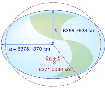
The Geospace environment is a region or neighborhood that is surrounding the Earth; it consists of Ionosphere, Plasmasphere (or Inner Magnetosphere), and Van Allen Radiation Belt, starting from 70 km above the Earth surface, and extending to about 10 R

E

(Earth radius). One R

E

is equal to 6,371 km, as explained in Figure 1-1; therefore, its

environment covered around 63,710 km from the surface of the Earth. Around the Geospace

environment is a matter of plasma state, plasma is the fourth state of matter, where the

particles are ionized (Maxworth, 2017). Major types of ions in the plasmasphere are protons,

helium ions, and oxygen ions and composition ratio of these ions plays an important role

in the propagation effect of VLF waves such as subprotonospheric whistler and

magnestospherically reflected whistler (Kimura, 1966). According to Miyoshi (2018), there

are several plasma and particle populations in the inner magnetosphere. The plasmasphere

consists of cold/dense plasma populations, and the ionosphere is the source of the

(15)

5

plasmaspheric plasma. Each region inside geospace environment has its own typical energy, which vary from 1 eV (plasmaspheric plasma), a few keV to about 100 keV (ring current and plasma sheet), a few hundred keV to more than 10 MeV (the radiation belt particle).

Thus wide energy range of plasma from a few eV to more than 10 MeV coexist in the inner magnetosphere.

Figure 1-1: Illustration of definition about 1 RE (Earth Radii). Image source: en.wikipedia.org

The three regions of geospace environment are shown in Figure 1-2. It consists of three region: Ionosphere, Plasmasphere, and Van Allen Radiation Belt. Different region has different characteristic and properties.

Figure 1-2: The Ionosphere is shown in orange, The Plasmasphere is light blue, and the Van Allen radiation belt is in red. Image source : (Compston, 2016)

(16)

6

According to Compston (2016), the ionosphere is consist of three different regions or layers: The D region, which starts at around 60 km, this region appear only during the day time. The E region, beginning at an altitude of about 90km up to 100km, and finally the F region, which extends up to 1000km beyond the E region.

The plasmasphere is a doughnut-shaped region above the ionosphere with closed magnetic field lines, it is filled from the dayside ionosphere and emptied to the night side through the ambipolar diffusion along field lines (Heilig, 2018). The upper side of the plasmasphere, known as the plasmapause, it extends to as many as three to seven Earth radii away from the planet (Compston, 2016). Plasma tends to be colder in this region (energies < 1eV), and the plasmapause marks the outer boundary of this region. Carpenter (1963) discovered the concept of the plasmapause, or the magnetospheric plasma knee, after an analysis of VLF whistler data showed a sudden change in the electron density decrease with increasing magnetic activity. This knee exists at all times in the magnetosphere.

Van Allen Belt, discovered by American space scientist James Van Allen, is a

region with an energetic charged particle within the cold plasma of the plasmasphere. There

is a population of energetic electron and proton (from ~100 keV to several MeV). Green

and Inan (2015), described Van Allen Belts consists of inner belt and outer belt. The inner

belt consists of high energy electrons between 0.04 MeV to 4.5 MeV; with altitude about

1,000 km up to L=3. Meanwhile, the outer belt extends from L=5 to L=7 and consists of

high energy electrons up to 7 MeV. Recent work from NASA Van Allen Probes Mission

(Baker et al., 2013; Selesnick et al. 2014) demonstrated that in the geocentric radial distance

of ~ 1.5 R

E

protons are quite stable with energies from ~10 MeV to~100 MeV. The

radiation belt is very important because it protects us from the harmful effect of high energy

particle radiation for human. The energetic particle is also responsible to the damage of

(17)

7

electronic equipment, such as induction of background noise in detector, error in digital circuit, degradation of electronic component particularly semiconductor and optical device.

Reviews on the inner magnetosphere and Van Allen belt can be found in several papers (e.q., Elkington, 2000; Ebihara and Miyoshi, 2011).

1.2 The Earth Magnetic Field

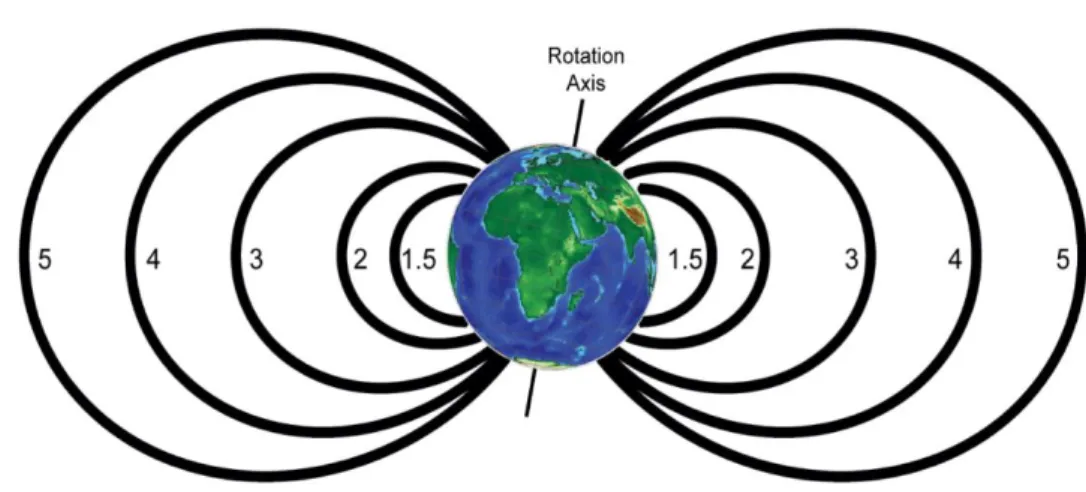
Figure 1-3: The concept of the L-Shell or L-Value or Mcllwain L-Parameter. Image source: vlf.stanford.edu

The Earth magnetic field, also known as the geomagnetic field, is dominant force

in the magnetosphere mostly caused by the Solar Wind. The Earth magnetic field can be

approximated by the field of magnetic dipole positioned near the center of the Earth. Its

dipole orientation is defined by an axis that best fits to the geomagnetic field intersect the

Earth’s surface which called as the North and South geomagnetic poles (Buffet, 2000). To

describe and measure a particular set of planetary magnetic field line or location in the

magnetosphere (Maxworth, 2017), we refer here to the L-shell value (L) and the magnetic

local time (MLT). The L-shell or L-Value, or Mcllwain L-Parameter as shown in Figure 1-

3 is a set of magnetic field line in the magnetic field model which crosses the Earth

magnetic equator at several Earth radii equal to the L-Value. For example, “L=3”, explains

the set of Earth magnetic field line which crosses the Earth’s magnetic equator three Earth

radii from the center of the Earth. L-shell is often used to describe the location of physical

(18)

8

phenomena that happen in the ionosphere and magnetosphere. While the MLT indicates the direction of the magnetic field relative to the direction of the sun and it’s occasionally referenced as UT-MLT to describe the offset between the temporal and MLT. The review on L-shell/L-values or Mcllwain parameter can be found at (Mcllwain, 1961).

1.4 ERG Satellite (ARASE)

The ERG (Exploration of energization and Radiation in Geospace) project is a mission to elucidate the acceleration and loss mechanisms of relativistic electrons in the inner magnetosphere during magnetic storms. It was launched at 20:00 JST on December 20, 2016, from Uchinoura Space Center (USC) in Japan with Epsilon-2 Launch Vehicle, with weight about 350 kg and an initial perigee and apogee of 440 km and 32,000 km, respectively. With the orbital inclination 31°, Arase satellite has wide latitudinal coverage, from the geomagnetic equatorial region until around the mid-latitude region.

Figure 1-4: Image showing the ERG mission, involving in situ measurements of the interactions between plasma waves and electrically charged particles in the Van Allen belts. Image source: (Miyoshi, 2018).

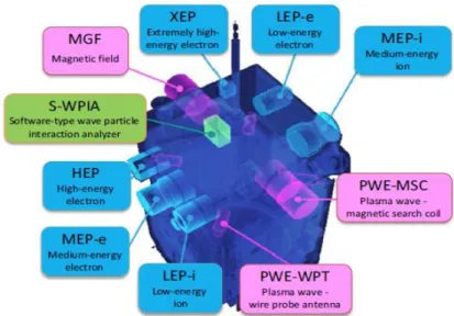
The Arase satellite has comprehensive in situ observations of plasma particles

(electrons and ions), fields and waves that are important to gather conclusive evidence of

(19)

9

wave-particle interactions driving high-energy electron acceleration. It has several major scientific instruments as shown in Figure 1-5 and 1-6 :

・ Low-energy particle experiments - electron analyzer (LEP-e)

・Low-energy particle experiments - ion mass analyzer (LEP-i)

・ Medium-energy particle experiments - electron analyzer (MEP-e)

・Medium-energy particle experiments - ion mass analyzer (MEP-i)

・ High-energy electron experiments (HEP)

・Extremely high-energy electron experiments (XEP)

・ Magnetic field experiment (MGF)

・Plasma Wave Experiment (PWE)

・ Software-type wave-particle interaction analyzer (S-WPIA)

Figure 1-5: Arase Satellite Scientific Instrument. Image source: (Nakamura, 2018)

(20)

10

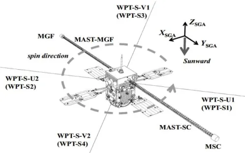
Figure 1-6: Configuration of the wave sensor and coordinate system of the Arase Satellite. The spin axis of the satellite was the Z-Axis and was always directed to the sun. Image source: (Kasahara, 2018)

1.5 The WFC (Waveform Capture)

The WFC (Plasma Wave Experiment - Waveform Capture), is one of the sub- systems of the PWE (Plasma Wave Experiment) on board the Arase (ERG) satellite. It measures waveforms below 20 kHz for the 2 electric field components and the 3 magnetic field components. The WFC is designed to measure chorus, hiss, and lightning whistlers.

Two kinds of operation modes, which are called chorus mode, and EMIC mode, are implemented. The chorus mode and EMIC mode are mainly operated around the apogee and perigee, respectively. The WFC data are stored as CDF files for easier data analysis.

 Chorus burst mode measures electric and magnetic field waveform at a high sampling rate (65,536 samples/s). Each sample consists of 2 bytes (131,072 bytes/s) with intermittently measured (8s/shot). This mode is designed for the wide-frequency range measurement of whistler-mode chorus emission, plasmaspheric hiss, and electron cyclotron waves.

 EMIC burst mode measures electric and magnetic field waveform at a low sampling

rate (1024 sample/s). Each sample consists of 2 bytes (2,048 bytes/s) with intermittently

(21)

11

measured (3min/shot). This mode is designed for the measurement of low-frequency phenomena such as EMIC waves and magnetosonic waves.

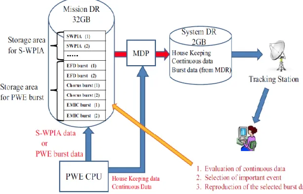
The burst data will be stored once on the Mission Data Recorder (MDR) and downloaded to the ground after data selection using the continuous data obtained by the OFA (Onboard Frequency Analyzer). The purpose of its measurements is to obtain entire ELF/VLF plasma wave activity and providing some properties such as power spectrum, propagation direction, and polarization for wave determination (Matsuda, 2018). The capacity of the MDR is 32 GB, which is allocated for EFD (Electric Field Detector), Chorus, and EMIC Burst. Figure 1-7 shows the data flow of the mission data and housekeeping data of the PWE. The burst data stored in the MDR are selected based on the evaluation of continuous data and selected data are reproduced to download to the ground.

Figure 1-7: Data flow of PWE housekeeping and mission data. Image source (Kasahara, 2018)

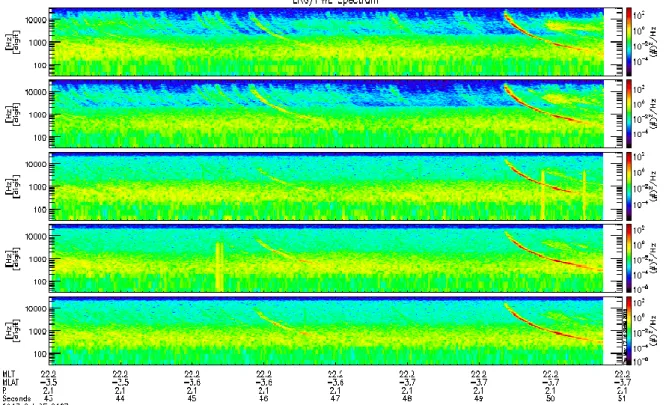
Figure 1-8 shows the 8-sec period of raw waveform data from the WFC

Arase/PWE instrument at 01:27:43 UT to 01:27:51 on October 25, 2017. In the figure, we

can observe raw data from 2 component of electric field (E1 waveform, and E2 Waveform),

(22)

12

and 3 component of magnetic field (Bα Waveform, Bβ Waveform, and Bγ). There is a raised intensity from 01:27:49 UT to 01:27:50 UT, which corresponds to a lightning whistler observed by the WFC. Since we cannot identify a lightning whistler wave on 1- Dimensional waveform signal as shown in Figure 1-8, whistler can be distinguished only on dynamic power spectra or spectrogram of a signal obtained by Hanning Window, FFT, and plot operation with contour by using IDL Procedure (TPLOT). Figure 1-9 shows the dynamic power spectra of the observed waveforms calculated using short-time Fourier transform (STFT) analysis with a 62.5-ms Hann window that included 4096 samples with a 94% overlap (shifting the window by 256 samples). The spectra shown here are not calibrated.

Figure 1-8: Raw data of the WFC waveform at 01:27:43 UT on October 25, 2017. There is a raised intensity from 01:27:49 UT to 01:27:50 UT, which in this case is the Lightning Whistler observed.

(23)

13

Figure 1-9: Dynamic Power Spectra produced by converting the WFC waveform data on Figure 1-8 using the Hanning Window and FFT Operation.

1.6 Purpose of the Present Work

The purpose of this work is to investigate lightning whistler observed by the WFC onboard Arase satellite in the following procedures, (i). Processing 1-year WFC data. (ii).

Generating dynamic power spectra plot from magnetic field component. (iii) Storing dataset of dynamic power spectra plot. (iv). Applying automatic lightning whistler to the dataset, and picking up the detected result. (v). Showing statistical result comparing with orbital data condition.

1.7 Thesis Organization

The present work is organized into 6 chapters:

In Chapter 1 (the current chapter) we introduce the background of the research, such

as the geospace environment, the Earth’s magnetic field, and the Arase (ERG) satellite

(24)

14

followed by the purposes of this study, and the structure of the thesis.

In Chapter 2, we explain the theoretical foundations. These include whistler lightning theory, dispersion, Earth-ionosphere waveguide propagation, atlas whistler, and occurrence of whistler.

In Chapter 3, we present an automatic whistler detection application to extract lightning whistlers from Arase observation data. We also demonstrate how it works.

In Chapter 4 we statistically analyze the detected whistlers extracted in Chapter 3, to investigate the spatial distribution, seasonal dependence, altitude dependence, MLT dependence, and MLAT dependence.

In Chapter 5, we present the result and discussion.

Finally, in Chapter 6, we summarize the results presented, compare these results

with related research, and conclude by proposing future work, including suggestions.

(25)

15

Chapter 2 Theoretical Background

2.1 Theory of Whistlers

Figure 2-1: Whistler wave formation, another part of electromagnetic radiation emitted by lightning is launched into the magnetosphere as a whistler wave. Image source: vlf.stanford.edu

When a lightning thunderbolt travels through the air, it doesn't just produce light and sound; it also creates radio-wave. Less than a second after lightning strike on the Earth, a radio-wave reaches the radiation belt where it interacts with electrically charged particles, as shown in Figure 2-1. A part of electromagnetic radiation emitted by a lightning discharge propagates in the Earth-ionosphere waveguide with the speed of light c. Ground and D- layer of the ionosphere are very good conductors in ELF/VLF range (300 Hz - 30kHz).

This part is called radio atmospheric of sferic for short. Another part of electromagnetic radiation emitted by lightning is launched into the magnetosphere as a whistler wave.

Because of its sounds like a “whistle.”, whistlers have characteristic as a radio signals in

the audio-frequency range that usually begins at a high frequency and in about one-second

drops to a lower limit frequency around 1 kHz (Helliwell, 1965).

(26)

16

Whistler is prominent in bursts of Very-Low-Frequency (VLF) electromagnetic energy produced by frequent lightning discharges. It propagates along the geomagnetic field lines from southern to northern hemisphere, and vice versa, as shown in Figure 2-2.

Dispersion of whistler indicates a gap of propagation delay in the frequency domain. Their spectral properties mainly depend on the plasma environments (electron density and ambient magnetic field) along their propagation paths, and it can propagate thousands of kilometers from the source of the lightning strike in the Earth’s plasmasphere. These data are relevant to the estimation of the electron density profile.

Figure 2-2: Propagation path of Lightning Whistler. It travels from northern hemisphere to southern hemisphere and vice versa following the geomagnetic field lines.

Whistler mode waves exist only in a magnetized plasma (Maxworth, 2016). The fundamental of this wave and the properties associated with the electromagnetic waves in free space are all electromagnetic phenomena derived from Maxwell's equations as shown in Equation (2.1):

∇ ∙ Ε =𝜌 𝜖

∇ ∙ Β = 0

∇ × Ε = −𝜕Β

𝜕𝑡

∇ × B = 𝜇𝜖J+𝜕𝜀Ε

𝜕𝑡

(2.1)

(27)

17

The E and B terms respectively refer to the electric and magnetic components of the wave, and the quantities 𝜌 and J correspond with the electric charge and the current densities.

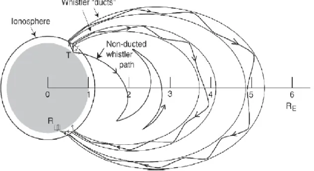
As the waves propagate through the plasma medium, they will propagate along the magnetic field lines called `ducts' which serves as guiding structure as shown in Figure 2-3. Since ducted waves arrive normal to the ionospheric boundary, all whistlers detected on the ground are considered to propagate in ducts. The plasma in the plasmasphere, in particular, the electrons, in the radiation belts interact with the waves in two different ways.

The low energy electrons in the plasmasphere support the propagation of waves at frequencies below the electron gyro-frequency in the whistler-mode, and generate a path delay and frequency dependent dispersion of the wave. The higher energy electrons in the radiation belts are much fewer in number and do not strongly affect the propagation of the wave but interact and exchange energy with the wave, resulting in wave amplification and the generation of new frequency components.

Figure 2-3: Electromagnetic wave propagation in the magnetosphere. Image source: vlf.stanford.edu

(28)

18

Whistler mode waves play a dominant role in the Earth's magnetosphere (Kulkarni et al., 2015). Figure 2-4 shows, the environment region where whistlers propagate. The most important parameters of the media that determine the propagation of whistler waves are electron number density (represented by color) and Earth’s magnetic field (field lines in black).

Figure 2-4: Whistler region of propagation. Image source: vlf.stanford.edu

2.2 Dispersion

Energy from a lightning discharge enters the ionosphere and is guided by the lines

of force of the Earth's magnetic field into the opposite hemisphere. As the radio waves

travel along this path, they are dispersed. Magnetosphere is dispersive; different

frequencies propagate at different group velocities. The wave in lower frequency arrives

later in time than the one in higher frequency. As mentioned above, we know that whistler

propagates through the plasma of the ionosphere and the plasmasphere before we know

complete description of whistler wave, we should understand how electromagnetic waves

propagate through a plasma environment. In general, the complex refractive index n of an

electromagnetic wave propagating through a homogenous plasma with a wave normal at

(29)

19

an angle from the ambient magnetic field is given by the so-called Appleton-Hartree’s equation given in Equation (2.2).

In Equation (2.2), the description of each equation symbol is:

c: Speed of light in vacuum.

k: Wave number.

𝜔: Radian frequency of the wave.

j = √−1 is the imaginary unit, and X, Y, and Z are, shown in Equation (2.3) :

ω

pe:

Plasma frequency.

Q

e:

Electric charge of an electron.

N

e:

Number density of electrons in the plasma.

ε

0

: Permittivity of free space.

m

e

: Mass of an electron.

ωce

: Gyro-frequency of an electron in an ambient magnetic field with strength B

0

. v: Collision frequency between electrons and other particles.

Equation (2.4) is a refractive index or dispersion relation derived from cold plasma model. W-k relation (dispersion relation) is shown in Figure 2-5. Taking into account the dispersion relation, from the result, we can calculate the group velocity of whistler mode – as shown in Equation (2.4). Refractive index or dispersion relation:

2 2

2

1 ( cos )

pe ce

kc 

     

 

       

(2.2)

(2.3)

(2.4)

(30)

20

This is a local group velocity at a specific point with specific plasma parameters. If it is integrated along the path of whistler waves, such as along magnetic field line, we can calculate the time delay for each frequency on the group.

Figure 2-5. Approximation of Whistler Wave Propagation. Image Source: vlf.stanford.edu

The group delay is with respect to the lightning discharge, with neglecting the propagation time in the Earth-ionosphere waveguide.

Group Velocity:

2

^ce

cos

g

pe

v c

k

 



  



2.3 Electron Density from Whistler Dispersion

Measurement of lightning whistler dispersion will help us to know the electron density distribution in the Earth’s Plasmasphere. It is well known that lighting whistlers propagate in ducts of plasma along the lines of the Earth`s magnetic field. There are many methods to measure the electron density; one of the methods is integral to the dispersion of whistler proposed by Gurnett et al. (1981). Bayupati (2012) applied this method using the principle of this approach. The time delay of the energy at frequency f during its propagation from one hemisphere to the opposite hemisphere is:

(2.5)

(31)

21

𝑡

_𝑑

= 1

2𝑐 ∫ 𝑓

_𝑝

𝑓

_𝑐

𝑓

^1/2

(𝑓

_𝑐

− 𝑓)

^3/2

𝑝𝑎𝑡ℎ

𝑑𝑠

where f

p

, f, f

c

and ds are plasma frequency, wave frequency, gyro-frequency and path length of the wave, respectively.

In order to derive time delay using this formula, we must follow this assumption:

1. cold plasma and the equations of magnetoionic theory;

2. there are no electron collisions;

3. the plasma is everywhere sufficiently dense so that f

p

>> f

c

; 4. positive ions are ignored

5. the wave normal is aligned parallel to the Earth`s magnetic field;

6. there are no effects from wave-particle interactions.

2.4 Arase Whistler Map

In 1965, Helliwell develops an Atlas of Whistler Spectra in order to describe whistler quantitatively. It includes the principal type of whistler, the range of variation within the type, intensity, fading, dispersion, cutoff frequencies, and diffuseness. We, however, newly proposed a definition of the type of lightning whistler observed by the Arase satellite and called it the Arase whistler map. This whistler map is partially adapted from the original definition of the whistler atlas defined by Helliwell (1965). The principal themes of the classification definition used in Helliwell’s whistler atlas were primarily based on ground observation result. For example, the difference between one-hop and two- hop whistler is the amount of relative dispersion, which depends on the length of propagation path. It was possible to distinguish one-hop and two-hop whistlers on ground- observations because the observation point is fixed. Such a classification is, however, not highly relevant for spacecraft observations because the observation point is always

(2.6)

(32)

22

changing. Particularly for the case of very elliptical orbit such as the Arase satellite, dispersion of lightning whistler drastically changes and it is impossible to distinguish one- hop and two-hop unless the location of wave source is identified. We classified the lightning whistlers based on the duration of the whistler trace instead, because the length of duration reflects the length of propagation path from the wave source to the observation point. In addition, we classified the multiple lightning whistlers according to the combination of the durations of the traces, which suggests the existence of multiple paths.

In this paper, we develop an improved detection method, based on pattern or shape

detection using image processing and image analysis approaches, via standard patterns by

measuring the pixel values, line groupings, and detected line in comparison to the shapes

in the reference atlas. The entire process runs concurrently, reading all the images at the

same time, detecting the whistler lines, and giving the results. As we can see in Table 2-1,

the Arase whistler map shows the spectral forms of the lightning whistlers and distinguishes

each type of whistler. We group the spectral forms into single-trace whistlers, which

include nose, short, middle, and long whistlers, and multi-trace whistlers, which include

the multiple-trace and multiple-combinations types. This grouping helps us formulate the

classification and detection algorithm described in the next section.

(33)

23

Table 2-1. Arase Whistler Map: Type & Principal Definition of Lightning Whistlers partially adapted from the original whistler atlas by Helliwell (1965).

2.4 Occurrence of Whistler

2.4.1 Diurnal variation Definition.

It is well known that whistler occurred mostly on the nighttime than during daylight hours. In this work, we will investigate this diurnal behavior in chapter 4 based on the result of detection in chapter 3. To demonstrate the diurnal behavior, we will measure the occurrence of lightning whistler for one complete year observation period; it will divide into quarters, based on calendar months, and centered approximately on the solstice and equinox period.

2.4.2 MLT Dependence Definition.

Lightning whistler tends to propagate through the ionosphere without attenuation at

night, while they are attenuated in the ionosphere in the daytime. Helliwell (1965) shows

the absorption amount of VLF waves as a function of geomagnetic latitude. Oike et al.

(34)

24

(2014) reported that lightning whistler rarely observed in the dayside, while the occurrence frequency becomes larger in the nightside.

2.4.3 Altitude Dependence Definition.

Lightning whistler, accompanied with the orbital position was examined. By

examining the time and location where each whistler was detected location/region of the

lightning whistler detected ins the plasmasphere (L-shell / L-value) can be investigated.

(35)

25

Chapter 3 The Lightning Whistler Detection Application

3.1 Observation

In this paper, we analyze the magnetic field data observed by the WFC in the chorus mode. We investigated lightning whistlers measured by WFC using the datasets of the magnetic field component. To generate a plot showing the variation of the frequency with time, we calculated the absolute value using the three components of the magnetic field waveforms.

|𝐵| = √𝐵

α2

+𝐵

β2

+𝐵

γ2

where Bγ is a spin axis component of a magnetic field vector and, Bα and Bβ are spin-plane components (Ozaki et al., 2018). To generate dynamic power spectra of the observed waveforms, we performed short-time Fourier transform (STFT) analysis with a 62.5-ms Hann window that included 4096 samples with a 94% overlap (shifting the window by 256 samples). The unit of a contour is an arbitrary unit/Hz (dB). The result of the dynamic power spectra were saved into an image file (PNG Format) which fits our monitor size resolution 1920 pixel x 1017 pixel.

(3.1)

(36)

26

Figure 3-1: An example of a frequency-time spectrum of lightning whistler with sferics and triggered emission observed from Palmer Station. Image source: vlf.stanford.edu

The relationship between the frequency and time of a lightning whistler, as seen in Figure 3-1, is theoretically explained by Eckersley’s law (Gurnett et al., 1990) which proves a simple relationship between the arrival time (t) of a lightning whistler at a frequency (f) as follows:

t = D /√f + t

0

where D is a constant value called dispersion of lightning whistler; t is the arrival time at a frequency f; and t

0

is the time when the lightning strikes. Bayupati et al. (2012) used the simple principle of Eckersley’s law on waveform data from AKEBONO to detect lightning whistlers. The conventional technique for the automatic detection of lightning whistlers is to identify straight lines in a diagram in which the dynamic power spectra are converted into a diagram with t on the horizontal axis and 1/√f on the vertical axis. The result of this technique is shown in Figure 3-2, where t1 and t2 are the arrival times of the detected lightning whistler at frequencies of f1 and f2, respectively. The dispersion D of lightning whistler is determined by detecting a straight line and deriving its gradient from Equation (3.3).

(3.2)

(3.3)

(37)

27

𝐷 = 𝑡

₂

− 𝑡

₁

1 √𝑓

₂

− 1

√𝑓

₁

It can be seen that the spectrum of lightning whistler appears as a straight line which is well marked by thick curves as shown in Figure 3-2. Equation (3.2) and (3.3), however, only explain the simple relationship between frequency and time for a subset of lightning whistlers; we cannot detect other types of lightning whistlers. The other types of whistlers shown in the whistler atlas compiled by Helliwell do not satisfy this equation. Accordingly, it is necessary to develop a new method to detect various types of lightning whistlers.

Figure 3-2: An example of a frequency–time spectrum of a lightning whistler observed on June 21, 1997, from AKEBONO, with the marked lightning whistler detected using the 1/√f conversion technique. Image source: Bayupati et al (2012)

(38)

28

3.2 Typical Shape of Lightning Whistler Observed by the WFC- Arase

There are several examples of lightning whistlers that were detected in the one-year

dataset from March 2017 to March 2018 observed by WFC onboard Arase. In this section,

we introduce the typical shapes of lightning whistlers observed by the Arase satellite and

compare them to the Arase whistler map; nose, short, middle, long, multiple-traces, and

multiple-combination whistler measured by Arase/WFC are shown in Figure 3-3. Because

we did not detect the source location or the direction path of the lightning whistler, we

classified the type based on only the shape or pattern representation of the lightning whistler

inside the spectrogram.

(39)

29

Figure 3-3: (a). Nose whistler at 10:44:27 UT on September 27, 2017; (b). Short whistler at 14:24:08 UT on October 02, 2017; (c). Middle whistler at 02:24:18 UT on September 14, 2017; (d). Long whistler at 02:26:22 UT on November 18, 2017; (e). Multiple-traces at 08:39:45 UT on September 07, 2017; (f). Multiple- combinations at 16:37:18 UT on October 09, 2017, observed by the PWE/WFC.

(40)

30

In the examples, as shown in Figure 3-3, the spectra were generated with the same period of (8 s) of data, where the X-Axis indicates time and the Y-Axis shows the frequency of the spectral observation. In the case of a single-trace whistler, we distinguished the type via its duration, except for the nose whistler because it has a unique shape. Meanwhile, for the case of short, middle, and long whistlers, we defined the type by its duration, as described in Table 2-1. In the case of multiple-traces and multiple-combinations whistlers, we checked the duration of each dispersion. When the whistler traces had the same duration, we called it a multiple-traces, whereas we called it a multiple-combinations when there were different durations. Because we only saw the whistler shape based on frequency and time points of detected whistlers, we compared the time delays of the whistlers relative to their pixel locations.

3.3 Flow of Detection

3.3.1 Pre-processing

To generate dynamic power spectra of the observed waveforms, we implemented a short-time Fourier transform analysis with a 62.5-ms Hann window that included 4,096 samples with a 94% overlap (shifting the window by 256 samples). The contour unit is an arbitrary unit/Hz (dB). To obtain a better detection result, we need a clear fine structure of the dynamic spectra of a lightning whistler with a high signal-to-noise ratio. The detailed performance of the magnetic search coil magnetic sensor can be found in Ozaki et al.

(2018). We applied a combination of filter operations using Gaussian filter. This technique eliminates the noisy pattern from the original spectra. To obtain the smoothing effectively, Gaussian smooth (also known as Gaussian blur) was implemented using a standard deviation sigma value of 𝜎 = 1.

𝑮

_𝝈⁼

𝟏 𝟐𝝅𝝈

^𝟐

𝒆𝒙𝒑 {− 𝒙

^𝟐

+ 𝒚

^𝟐

𝟐𝝈

^𝟐

}

(41)

31

To generate a clear fine structure from the edge detector, we applied a Laplacian operation to compute the second derivative of the image resulting from the Gaussian blur.

Figure 3-4 shows an example of the dynamic spectra of a magnetic field observed at 02:24 UT on September 14, 2017. The upper panel shows the dynamic spectra processed from the WFC data, and the lower panel shows the edge spectra after using Gaussian blur and Laplacian filtering to remove noise. As can be seen in the upper panel, the clear fine structure of the lightning whistler is characterized by a discrete tone that decreases in frequency with increasing time. The bottom panel shows the clear result of a whistler trace in the dynamic spectra after implementing the Gaussian blur and edge detection via the Laplacian filter. We then performed the above-mentioned pre-processing on the result of the dynamic power spectra and saved it to an image file (PNG format) that fit our monitor size resolution of 1920 × 1017 pixels. The saved file has the same information as shown in Figure 3-4. This file was then used as input for our detection system. The total number of spectral image data files produced during the observations is shown in Table 3-1.

Figure 3-4: (top) The original middle whistler dynamic spectra observed at 02:24:17 UT on September 14, 2017. (bottom) Edge spectra after using a Gaussian blur with a mask (1,0.1) and Laplacian filtering to remove noise

.

(42)

32

Table 3-1. Total numbers of the spectra image file as a function of month.

Year 2017 2018

Month Mar Apr May Jun Jul Aug Sep Oct Nov Dec Jan Feb Mar

Total Files 2102 649 2088 3209 2319 2205 5027 3378 3021 1696 2153 2163 1370

3.3.2 Overview of the Detection System

Figure 3-5 shows the overall flow chart of our proposed whistler detection method.

The quality of the input image of the candidate area directly affects the accuracy of the target detection task. We have two different spectra (original and pre-processed), as shown in Figure 3-4. To extract information from the input image, our detection system only uses the segmented input image from the pre-processed spectra. This operation not only accelerates the speed of target detection but also improves the detection performance because the information has a clear fine structure with the unwanted information eliminated (e.g., the attached noise).

Figure 3-5: The overall flow chart of the whistler detection system. The process from left to right shows segmentation, extraction of the candidate area, the classification rule, and the detection result.

(43)

33

The segmentation target area indicates an area with an important detection where a lightning whistler is located. We define a partitioned area inside this area, then split it into grid lines, as shown in Figure 3-6. Each grid line represents information about the time and frequency. The X-axis represents the time of the observation with 100-ms increments. The Y-axis represents the frequency on a logarithmic scale. Then, we calculate the average of each pixel point for every represented grid point. We limited the detection frequency range from 1 kHz to 20 kHz. The segmentation result of the image grid of the target area was produced using the OpenCV function and the neighboring pixel relation (N8). Groups of pixels of the binary image with similar features (colors) are obtained, in which the whistler region is 1 (non-white) and the non-whistler region is 0 (white). Subsequently, we used Bresenham’s line algorithm (Bresenham, 1977) for every step after segmentation, from line grouping, line detector, and line counter. Bresenham’s algorithm is a widely used high- speed algorithm that rasterizes straight lines/circles/ellipses using only addition and subtraction operations of pure integers; description and the concept of this algorithm is available in Bresenham (1977).

Figure 3-6: The segmentation of the input image shows in the 4-sec duration of observation into a grid line to corresponding pick-up information.

(44)

34

The process of line grouping starts from a neighboring pixel that is connected with the Bresenham function; then the pixels are grouped as a line group. Further, the area of the adjacent neighboring block is scanned with triangular scanning to locate the boundary.

The checked block is eliminated and then another block is moved to that is already marked as a line group. After the line group is connected, we add labeling for each starting and ending point of the line group associated with the pixel position of the grid corresponding to time on the X-axis and frequency on the Y-axis. Examples of detected lines are shown in Figure 3-7. Then, the detected lines are analyzed one by one as whistler traces: single lines that represent a whistler. There are two types of whistler traces: single traces and multi-traces. The system marks each starting and ending point (x, y) of the whistler trace, compares its location based on the pixel grid, and stores the corresponding information.

The X-axis (time) indicates the duration of the lightning whistler, and the Y-axis indicates its frequency.

Figure 3-7: The result of the detected line and grouped as line-group.

Figure 3-8 shows the application interface of the detection system with the case of

single detection. Figure 3-9 shows the detection of the case of bulk detection with the queue

status of the input image on the target folder, and Figure 3-10 shows the interface of result

from the bulk detection process.

(45)

35

Figure 3-8: Overview of lightning whistler detection application; the case of single detection image spectra.

Figure 3-9: Overview of whistler detection application with the bulk detection process (queuing list)

(46)

36

Figure 3-10: Overview of lightning whistler detection application; the bulk detection process (detail view)

According to the Arase whistler map, there is one type of whistler that is distinguished by a different shape than the others, the nose whistler. The others have the shape of a normal whistler and are either single-trace or multi-trace whistlers. The duration of lightning whistlers as well as their combination is important when deciding the type of lightning whistler propagating in geospace.

We developed a classification rule and principle, in which the nose whistler is

checked for before the other types are detected. The detection process starts with line-group

counting. If no line groups exist, the event is identified as no-whistler. If a line group exists,

the next step is to determine if it complies with the nose whistler check criteria. If yes, then

we mark it as a nose whistler. If we fail to detect a nose shape, then we check the number

of line traces in the line-group process, we categorize it as a single-trace or multi-trace

whistler, and then we check the duration of each trace line detected. The event will then be

classified based on the rules that can be summarized as shown in Figure 3-11.

(47)

37 Figure 3-11: Decision tree for the all-whistler classifier.

To successfully detect a nose whistler, we define a criteria-matching region as

shown in Figure 3-12. The explanation of this region is as follows. The black line is an

example of a nose whistler existing in a diagram of the dynamic spectra. It has a starting

point, which is marked as XsYs and an ending point marked XeYe. As a reference of the

Cartesian axis, the orange line represents the Y-axis (frequency) and the purple line

represents the X-axis (time). The green region is located to the left of the Y-axis, and the

blue region is located to the right of the Y-axis. These two regions will help us determine

whether the component of the targeted whistler trace/whistler line belongs to the criteria

matching a nose whistler.

(48)

38 Figure 3-12: Nose-whistler detection criteria-matching region

We developed an algorithm to check for nose whistlers first; this algorithm is the first step before we can successfully detect all other types of lightning whistler. The pseudo code and detailed detection of a nose whistler are described in Algorithm 1.

Algorithm 1: The Nose-Whistler Detection Algorithm 1 For each line group in the image

2 Find the maximum frequency and time on the X-axis and Y-axis (XsYs) 3 var Ys = line_group.Min(s => s.point.Y);

4 var Xs = line_group.Where(s => s.point.Y == Ys).Min(s => s.point.X);

5 Find the lowest time point on the X-axis 6 var left_x = line_group.Min(s => s.point.X);

7 Find the lowest frequency point on the Y-axis

8 var left_y = line_group.Where(s => s.point.X == left_x).Max(s => s.point.Y);

9 Compare the pixel location region of the starting time 10 if (left_x >=Xs)

11 return false;

12 Compare the pixel location region of the whistler trace in the green region

13 if ((left_x <= Xs - (1 * line_group.neighborInterval) && left_y - Ys >

(49)

39

14 line_group.neighborInterval + 1) == false) 15 return false;

16 Find the lowest frequency point of the start point of the whistler trace on the Y-axis 17 var bottom_y = line_group.Max(s => s.point.Y);

18 Find the lowest frequency point of the last point of the whistler trace on the Y-axis 19 var bottom_x_fr_bottom_y = line_group.Where(s => s.point.Y == bottom_y).Max(s

=> s.point.X);

20 Compare the pixel location region of the whistler trace in the blue region

21 if(bottom_x_fr_bottom_y >= Xs + (1 * line_group.neighborInterval)) == false) 22 return false;

23 Detection result

24 whistler.type = WhistlerModelType.Nose;

25 return true;

3.4 Experimental Result and Analysis

To evaluate the performance of the proposed method, we tested a set of real images of

dynamic spectra produced by WFC. The entire experiment was performed on a Core-i7-

4810 MQ 2.8 GHz (8 CPUs) with 16GB of RAM. Before processing the entire dataset, we

tested the detection algorithm for each type of lightning whistler, as can be seen in Figure

3-13 and Figure 3-14. The detected whistler is traced by a box, and the result of each

detection is stored in a text file with each characteristics such as type, start time, end time,

start frequency, end frequency, and time consumed for each detection process. Some

whistlers were not detected due to the density between pixels. We rely on the concept of

the neighboring pixel, so if the filtering in the pre-processing results in a weakly connected

or un-connected line, this will affect our detection system. The event will not be detected

(50)

40

as a line because it is not a single connected line. To prevent this and improve the detection accuracy, it is necessary to develop an intermediate process between spectral filtering and detection. This process should make adjustments to maintain the pixel quality, prevent pixel loss, and refine connected lines to improve the detection process and increase the accuracy.

Figure 3-13: The detected nose, short, middle, and long whistler types.

Figure 3-14: The detected multiple-trace and multiple-combination whistler types.

For comparison with the algorithm result, we used “manual inspection” that we

made a year before we developed this application, that is, we conducted a direct inspection

to identify all the available image spectra. In this observation, we visually inspected, one

by one, every image spectra and investigated the detected lightning whistlers via the

(51)

41

spectrogram. Because this type of observation depends solely on the experience of the investigator, the manual inspection took a long time and we checked every detail of each spectrogram and carefully marked the event and type using the principles defined in the Arase whistler map. In our detection policy for automatic detection, we prioritize highest accuracy of false-detection. False-detection means that shape of lightning whistler trace is inappropriately detected and thus differently classified because of the background noise.

To decrease the false-detection rate, a higher threshold level is necessary, but it causes an increase in mis-detection rate. Here mis-detection means that weak lightning whistler cannot be detected due to faint and patchy line that fails line grouping by the Bresenham’s line algorithm. Using optimized parameters, we performed bulk processing of detection for one-year data. To use our proposed algorithm, we loaded all the images as input into the application and the application processed each detection concurrently with the available CPU and memory. It took 30 h to completely detect all the whistlers in the available dataset.

Some whistlers were not detected due to our detection policy. The result of the detection

system as output from the application is shown in Table 3-2. There are 711 image files in

which we could detect lightning whistlers, while 1,165 of line groups were identified

among the 711 image files. We couldn’t detect any long whistlers when we apply the

optimized parameter. In fact, we can detect a long whistler as shown in Figure 3-13, if we

optimize the parameter only for this event, but it causes an increase of false detection rate

for the other events due to contaminated noise.

(52)

42

Table 3-2. The comparison detection result using the defined algorithm and manual inspections.

We assume that the manual inspections are more reliable than the automatic detection because the algorithm still has a limited capability and further work needs to be done to improve it, such as selecting different types of filtering to improve the quality of the input image in the pre-processing and to increase the detection accuracy. By detecting whistler using duration approached, our classification system has decreased the number of false classification. False classification mean that the system classified the wrong type of lightning whistler within the same criteria. It probably happens when the false line detected as lightning whistler. In the Table 3-2, we show that we couldn’t classify the long whistler.