JAIST Repository: A study on sentiment classification with LSTM+GRNN and Sub-tree Mining

全文

(1)JAIST Repository https://dspace.jaist.ac.jp/. Title. A study on sentiment classification with LSTM+GRNN and Sub-tree Mining. Author(s). Chau, Ngoc Phuong. Citation Issue Date. 2016-09. Type. Thesis or Dissertation. Text version. author. URL. http://hdl.handle.net/10119/13742. Rights Description. Supervisor:NGUYEN, Minh Le, 情報科学研究科, 修士. Japan Advanced Institute of Science and Technology.

(2) A study on sentiment classification with LSTM+GRNN and Sub-tree Mining. CHAU, Ngoc Phuong School of Information Science Japan Advanced Institute of Science and Technology September, 2016.

(3) Master’s Thesis. A study on sentiment classification with LSTM+GRNN and Sub-tree Mining. 1410217 CHAU, Ngoc Phuong. Supervisor : Associate Professor Nguyen Minh Le Main Examiner : Associate Professor Nguyen Minh Le Examiners : Associate Professor Kiyoaki Shirai Professor Satoshi Tojo. School of Information Science Japan Advanced Institute of Science and Technology August, 2016.

(4) Contents 1 Introduction 1.1 Motivation . . . . . . . . . . . . . . . . . . . . . . . . . . . . . . . . . 1.2 Goal . . . . . . . . . . . . . . . . . . . . . . . . . . . . . . . . . . . . 1.3 Thesis Outline . . . . . . . . . . . . . . . . . . . . . . . . . . . . . . . 2 Background 2.1 Sub-tree Mining . . . . . . . . . . . . . . . . 2.1.1 Tree Concepts . . . . . . . . . . . 2.1.2 Mining Frequent Sub-tree . . . . . . 2.2 Sentiment Classification . . . . . . . . . . . 2.3 Sentiment Classification with Deep Learning 2.4 Summary . . . . . . . . . . . . . . . . . . .. . . . . . .. . . . . . .. . . . . . .. 3 The proposed model 3.1 Sentence Representation . . . . . . . . . . . . . . 3.2 Frequent Sub-tree Mining, Outlier Detection . . . 3.2.1 Frequent sub-tree mining . . . . . . . . . . 3.2.2 Outlier detection . . . . . . . . . . . . . . 3.3 Representing Frequent Tree or Frequent Sub-tree 3.4 LSTM + GRNN . . . . . . . . . . . . . . . . . . 4 Evaluation 4.1 Corpus . . . . . . . . . . . . . . . 4.1.1 Multi-Domain dataset. . . 4.1.2 Yelp 2013 dataset. . . . . 4.2 Evaluation Methods . . . . . . . 4.2.1 Accuracy evaluation . . . 4.2.2 Mean Square Error (MSE) 4.3 Experiment Settings . . . . . . . 1. . . . . . . . . . . . . . . . . . . . . . . . . . . . . . . evaluation . . . . . .. . . . . . . .. . . . . . . .. . . . . . . .. . . . . . .. . . . . . .. . . . . . . .. . . . . . .. . . . . . .. . . . . . . .. . . . . . .. . . . . . .. . . . . . . .. . . . . . .. . . . . . .. . . . . . . .. . . . . . .. . . . . . .. . . . . . . .. . . . . . .. . . . . . .. . . . . . . .. . . . . . .. . . . . . .. . . . . . . .. . . . . . .. . . . . . .. . . . . . . .. . . . . . .. . . . . . .. . . . . . . .. . . . . . .. . . . . . .. . . . . . . .. 6 7 8 8. . . . . . .. 10 10 11 12 15 17 18. . . . . . .. 20 21 22 22 24 27 27. . . . . . . .. 30 30 30 31 31 31 33 33.

(5) 4.4 4.5 4.6. Results . . . . . . . . . . . . . . . . . . . . . . . . . . . . . . . . . . . Results Analysis . . . . . . . . . . . . . . . . . . . . . . . . . . . . . . Error Analysis . . . . . . . . . . . . . . . . . . . . . . . . . . . . . . .. 34 35 36. 5 Conclusions and Future Work 40 5.1 Conclutions . . . . . . . . . . . . . . . . . . . . . . . . . . . . . . . . 40 5.2 Future Work . . . . . . . . . . . . . . . . . . . . . . . . . . . . . . . . 41 This dissertation was prepared according to the curriculum for the Collaborative Education Program organized by Japan Advanced Institute of Science and Technology and Vietnam National University - Ho Chi Minh City.. 2.

(6) Acknowledgements First of all, I would like to express my gratitude to Associate Professor Nguyen Minh Le who is my supervisor and always gives me pieces of advice to complete my thesis on time. Secondly, I would like to thank Associate Professor Kiyoaki Shirai who is my co-supervisor of this master course. Next, I would like to thank Professor Satoshi Tojo who is an examiner in midterm defence gives me some advice to improve this thesis. I would like to thank the teachers at Vietnam National University - Ho Chi Minh City and JAIST who gave me the necessary basic knowledge so that I can finish this thesis. Besides that, I would like to give thanks to Associate Professor Le Hoai Bac who always give me a huge encourager of my research. Finally, I would like to thank my family, all member of Nguyen laboratory and my friends who are friendly, gives me a big inspiration.. 3.

(7) List of Figures 1.1. The process of SC problem. . . . . . . . . . . . . . . . . . . . . . . .. 2.1 2.2 2.3 2.4 2.5 2.6. An example tree. . . . . . . . . . . . . . . . . . . . . . . . . . . . . Two sub-tree in the tree in Figure2.1. . . . . . . . . . . . . . . . . . Candidate Generation. . . . . . . . . . . . . . . . . . . . . . . . . . a) binary classification b) multiple classification. . . . . . . . . . . . The repeating module in a standard RNN contains a single layer. . The repeating module in an LSTM contains four interacting layers.. . . . . . .. 11 13 15 16 17 18. 3.1 3.2 3.3 3.4 3.5 3.6. An overview of our model. . . . . . . . . . . . . . . . . . . . . . An example about sentence representation by tree. . . . . . . . The sample dataset of frequent sub-tree mining. . . . . . . . . . The frequent sub-trees of dataset in Figure 3.3 with minsup = 2. An example of applying FindBestSub-tree algorithm. . . . . . . LSTM+GRNN model [22]. . . . . . . . . . . . . . . . . . . . . .. . . . . . .. 21 23 24 25 27 29. 4. . . . . . .. . . . . . .. 6.

(8) List of Tables 3.1. FindBestSub-tree algorithm . . . . . . . . . . . . . . . . . . . . . . .. 26. 4.1 4.2. Characteristic of the experimental datasets . . . . . . . . . . . . . . . The average number of frequent sub-tree in 10-fold with minimum support - Multi-Domain dataset . . . . . . . . . . . . . . . . . . . . . The average number of frequent sub-tree in 10-fold with minimum support - Yelp 2013 dataset . . . . . . . . . . . . . . . . . . . . . . . Sentiment classification on Multi Domain Dataset. The best results are in bold. Acc is accuracy, and MSE is mean squared error. . . . . Sentiment classification on Yelp 2013 Dataset. The best results are in bold. Acc is accuracy, and MSE is mean squared error. . . . . . . . . Some examples in sentiment classification between our model and LSTM+GRNN model. Doc is Document. . . . . . . . . . . . . . . . .. 32. 4.3 4.4 4.5 4.6. 5. 35 36 37 38 39.

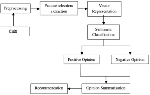
(9) Chapter 1 Introduction In sentiment classification (SC) problem, it has a large number of challenges, and one of the challenges is how to find relevant features for machine learning models. Beside that, this is also an essential task for improving the accuracy of sentiment classification. In figure 1.1, This is an overview of phases in SC. Firstly, text data which is collected from comments or product reviews is processed to get significant information. Secondly, features from text data are selected. Next, these features are represented by real value vectors. Finally, A machine learning method is used for training and testing the data.. Figure 1.1: The process of SC problem. 6.

(10) The tree is a structure that used in a lot of fields in machine learning. Sub-tree mining is a suitable method for classification in machine learning [12] [19]. In natural language processing, the tree is also an approach such as parser tree that is based on grammar tree. In this thesis, we used Stanford Parser 1 to parse sentences to trees. Hence, sub-tree mining is a good method to find all features of a parse tree and detect outliers before training or testing phase. However, this is not an easy task. We want to investigate some estimation methods for selecting appropriate sub-tree features. Another significant problem is how to choose a suitable machine learning method for training with sub-tree mining. Deep learning is a part of machine learning and develops rapidly over the past five years, and it is the top of trends in machine learning. In addition, LSTM + GRNN achieved high accuracy in many natural language processing application [22] [14]. Therefore, we decided using Long ShortTerm Memory + Gated Recurrent Neural Network (LSTM + GRNN) for training after feature selection phase.. 1.1. Motivation. Recently, with the development of the online social network, the determination of opinion of people which is called sentiment classification becomes a significant task in natural language processing. From the identification of the positive or negative comments, sentiment classification can determine the number of stars in a product review. However, many reviews from customers are not correct such as spam comments or spam reviews. The determination of spam comments or spam reviews is also a big challenge in this task. Besides that, in the research of sentiment classification, it is still many challenges like as how to represent the semantic relation among words in a sentence, among sentences in a document, how to select significant features, remove outliers, etc. These challenges are not an easy task in natural language processing and machine learning. Therefore, this is an essential problem for understanding as the human of the computer. In general, sentiment classification problem has three level. According to the target of sentiment or level of the text, the task belongs to word/phrase level, sentence level or document level. In sentiment classification, document level is very complexity, so this level seems to a big challenge in sentiment classification problem, and it is also the target of our model. 1. http://nlp.stanford.edu/software/lex-parser.shtml. 7.

(11) 1.2. Goal. Statistical machine learning model and deep learning model have widely applied in a lot of fields in computer science such as data mining, bioinformatics, computer vision and natural language processing (NLP). In NLP field, both statistical and deep learning model is applied in the various problems such as machine translation, question answering, summarization and SC problem. However, it remains challenges to improve these efficient models. In this thesis, the research aim is that the semantic of the words in sentences is considered, and the structure of sentence tree is also mentioned to improve the accuracy in sentiment classification problem. In our model, the combination of data mining and deep learning is shown an efficient model in SC problem. Our model is divided into four step. Firstly, Stanford dependency parser illustrates the semantic relation among words in a sentence to create a dependency tree. Secondly, sub-tree mining is used for determining and eliminating outliers from the data. Next, a tree after outlier detection phase is represented by a string of words. Finally, a deep learning model is used for training and testing phase. In this thesis, this model is used for improving the performance in SC problem and proposed method achieved improvements in term of accuracy in a range of 0.14% 6.93% over LSTM + GRNN model.. 1.3. Thesis Outline. This thesis has five chapters such as Introduction, Background, Proposed Model, Evaluation, Conclusion and Future Work. The structure of dissertation is discussed as follows. In Chapter 2, we introduce different background knowledge related to related our research. At first, basic concepts about graph and tree are shown with examples. Then, we describe some definitions of SC problem and show some studies in SC problem. Finally, any studies in SC problem with deep learning are illustrated to show the combination deep learning in this task. In Chapter 3, we describe the proposed model. Then, we will show basic definitions and notations in the model. Next, we will introduce about details of parts in our model. Finally, each part with the examples are presented techniques in the subsection. In Chapter 4, we show the characteristics of the Multi Domain dataset, Yelp 2013 dataset and experiment setting in our model. Then, we describe measure for evaluation. Next, we discuss results of the analysis with any minsup parameters. 8.

(12) Finally, some examples which are improved in our model than LSTM+GRNN model are shown. In Chapter 5, the brief statements of the main point and future work are discussed in this section.. 9.

(13) Chapter 2 Background In this chapter, we cover basic background and some related works. Firstly, some definitions and examples in sub-tree mining are introduced. Secondly, sentiment classification related work is shown with the development of machine learning methods. Finally, any definition of deep learning and deep learning model for SC problem are analysed.. 2.1. Sub-tree Mining. Tree structure was used commonly in data mining and machine learning, and sub-tree mining is suitable for classification on machine learning [12], [19]. The approach using tree structure is common in natural language processing, especially, dependency tree based on grammar structure. Hence, sub-tree mining is a proficient method to find all features from parse trees for training. However, this is challenging and requires some further studies for selecting appropriate sub-tree features. Sub-tree mining [1], [25] is one of the methods in data mining for finding frequent trends and outliers from the dataset. In outlier detection, E. M. Knorr [11] introduced an algorithm for mining distance-based outliers in large datasets in 1998. After that, a lot of algorithms were proposed for outlier detection such as S. Ramaswamy [18] with Efficient Algorithm in 2000, M. M. Breunig [4] with Identifying Density-Based local outlier. Especially, in April 2016, Zengyou He [8] used frequent patterns for outlier detection. In this section, we provide necessary concepts about tree sub-tree and sub-tree mining. We first give an overview of basic definitions in tree theory. Moreover, then, we discuss sub-tree and how to generate candidates for sub-tree without isomorphism. Finally, we introduce mining frequent sub-tree.. 10.

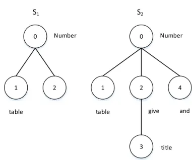
(14) 2.1.1. Tree Concepts. Number. table. all. and. give. figure. each. and. title. a Figure 2.1: An example tree. Tree is a data structure which including nodes (or vertices) and edges without cycle. Null tree or empty tree is a tree with no node. Root is a top node of a tree in the non-empty tree. Edge is a direct link from a node to another node. Child node and parent node are two nodes which connected by an edge. The node with the nearest from the root is parent node, and the other is child node. Siblings are many nodes with the similar parent node. Leaf is a node without child node. Degree of a node is the number of sub-trees of a node. 11.

(15) Path between two nodes in a tree is a sequence of nodes and edges to connect the two nodes. Level of a node N is defined by 1 + (the number of edges in the path from root to node N) Height of tree is the longest path from root node to leaf node. A Forest is a set of n trees (n ≥ 0). k-subtrees of a tree T is a set of trees with k nodes and k 1 ≤ k ≤ n (where n is the total nodes in T). From a sentence “Number all tables and figures and give each a title”, Figure 2.1 shown a sample dependency tree after using Stanford dependency parser. The tree includes ten nodes (Number, table, give, and, all, and, figure, each, title, a) and nine edges. Node “Number” is a root node. To consider child node and parent node concept, while “Number” node is the parent node of “table” node, “give” node and “and” node, “table” node, “give” node and “and” node are the child node of “Number” node. Siblings set of “table” node is “give” and “and” node. The leaves of the tree are “all”, “and”, “figure”, “each”, “a” and “and” node. The degree of “give” node is one because we have only one sub-tree “title”-“a” (in this case, “each” node is not sub-tree due to no edge by one node).. 2.1.2. Mining Frequent Sub-tree. In my thesis, three main parts are considered such as problem, representing a tree as a string of words and generating candidate. In the issue, the concepts of sub-tree mining are defined formally. Next, to repair for generating candidate phase, a tree is represented by a string with the definition of Zaki [26]. Finally, the details of creating candidate are discussed in generating candidate phase.. Problem In data mining, frequent sub-tree mining is a problem which determines all subtrees in the database within a minimum support (minsup) threshold. Formally, the definition of sub-tree mining is defined as: Given a threshold minsup, find all trees or sub-trees with support is equal or greater than minsup.. 12.

(16) where support is defined as the number of occurrences of a tree or sub-tree in dataset D = {T1 , T2 , ..., Tn } and the support of a tree or sub-tree is defined as: support(Ti ) =. #Ti |D|. (2.1). where #Ti is the number of advents of tree Ti in dataset D and |D| is total trees in D.. Resenting Tree as String. S1 0. 1. table. S2 Number. 2. 1. 0. Number. 2. 4. give. table. 3. and. title. Figure 2.2: Two sub-tree in the tree in Figure2.1. For representing tree as a string, Zaki [26] adopted a tree by a string. The string of a tree T was denoted T . Firstly, T = ∅. A depth-first pre-order search is started at the root, added extended node x to T. When backtracking from a child to its parent, a unique symbol “- 1” is added to the string. By this way, the represented tree with an arbitrary number of children from a parent node is convenient, and resenting tree as a string is simpler than adjacency list. The notation l(T ) is the label sequence of T, which includes the node labels of T in depth-first ordering. 13.

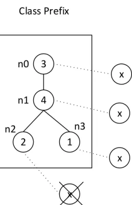
(17) Figure 2.2 is two subtree in the tree in Figure 2.1. To address the encoder the tree by string, we consider two sub-tree S1 and S2 . For example, sub-tree S1 and S2 are encoded by the string “0 1 -1 2 -1” and “0 1 -1 2 3 -1 -1 4 -1”, respectively. In the string of S1 , T = ∅, starting at root node with label 0, we add node 0 to the string and T = 0. The next node is label 1, which adds to the string and the string is “0 1”. Then, the node 1 has no child node, and we backtrack to the parent node, so the string is “0 1 -1”. after that, the node two is added to the string. Finally, we backtrack to the root node and add “-1” to the string. Therefore, the string of S1 is “0 1 -1 2 -1”. Note that the label sequence of the S1 is “0 1 2”. Similarly, the string and the label sequence of S2 are “0 1 -1 2 3 -1 -1 4 -1” and “0 1 2 3 4”, respectively.. Generating Candidate In dataset D, there is two main step to finding all frequent sub-trees. Firstly, the candidate was generated, which maintained non-redundant, and each sub-tree should be created as most once. Secondly, The number of occurrences of each candidate in the database D are counted to find out all candidates with support ≥ minsup threshold. Candidate generation procedure [26] used the anti-monotone property of frequent patterns to generate candidates. It is mean that the frequent of sub-tree is greater than or equal to the super-tree (parent tree). Therefore, the extension of the frequent pattern is considerable. At the time, an extension by a single node is more efficient. Thus, the candidate (k+1)-subtrees are generated by the information of k-subtrees. Equivalence Classes Considering two k-subtrees X and Y, there are similar prefix equivalence class if and only if they share a common prefix up to the (k − 1)th node. Therefore, X and Y are only different at the last node. Figure 2.3 shown that some subtrees with five nodes were created by a subtree with four nodes. The string encoding of sub-tree with four nodes is P = 3 4 2 -1 1, and “x” is a label from label set (L). With prefix P, the valid positions for the node with label x are n0, n1 and n3 because the string encodings of the tree in with these positions are the same prefix P. On the contrary, with the position n2, the prefix of string encoding is different from P, given as 3 4 2 x. The figure 2.3 also shows the format Zaki uses to represent an equivalence class. It includes the prefix string and a list of elements. A(x,p) pair is an element with label x of the last node and the depth-first position p of the node in P to attach x. Given an equivalence class of (k-1)-subtrees. We consider how to generate candi-. 14.

(18) Class Prefix. Equivalence Class n0. 3. n1. 4. Prefix String: 3 4 2 -1 1. x. Element List: (Label, attached to position). x. (x,0) // attached to n0: 3 4 2 -1 1 -1 -1 x -1 (x,1) // attached to n1: 3 4 2 -1 1 -1 x -1 -1 (x,3) // attached to n3: 3 4 2 -1 1 x -1 -1 -1. n3. n2. 2. 1 x. x. Figure 2.3: Candidate Generation.. date k-subtrees. Firstly, with the elements (x,p) in the equivalence class, sorting by node label is implement with node labels as primary key and position as the second key. Secondly, from the sorted elements, the candidates is generated by adding elements (x,p) into (k-1)-subtrees. The extended (x,p) pair is the main idea of this algorithm.. 2.2. Sentiment Classification. SC or opinion mining is a task of natural language processing which analyses and classifies documents into categories according to people’s opinions. In general, this 15.

(19) problem has three level such as word/phrase level, sentence level and document level. In this thesis, the document level is the target of our model because of the complexity of this problem. Sentiment classification technique was proposed by Pang [16] in 2002, which employed Naive Bayes and SVM. Then, Centroid Classification and KNN [21], for example, were developed. From text data, the output is shown only positive or negative labels. These methods are based on statistical classification. At document level, Turney [23] introduced a method that used information from words/phrases to extract opinion of users to determine positive or negative text. Then, sentiment classification was developed by Pang [15] in 2005. Goldberg and Zhu [7] used a graph-based method in 2006 to solve sentiment classification problem. Thereafter, a wide range of models were used for sentiment classification such as word n-grams [24], text topic [6], bag-of-opinions [17], etc.. (a). (b). Figure 2.4: a) binary classification b) multiple classification.. The Figure 2.4 shows binary classification and multiple classifications in sentiment classification. While Figure 2.4a is an example of like or dislike classification, Figure 16.

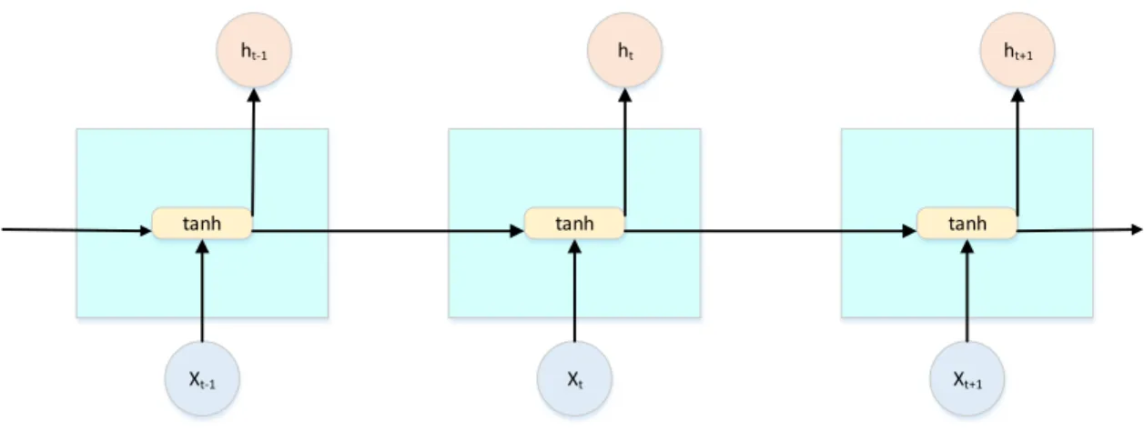
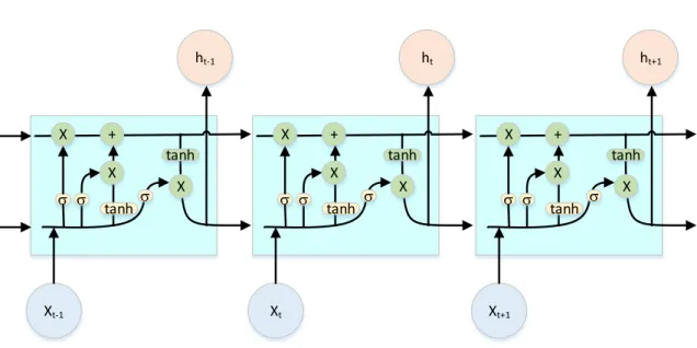
(20) 2.4b is a case of the number of rating classification (from one to five stars).. 2.3. Sentiment Classification with Deep Learning. With the development of deep learning, Shusen Zhou (2010)[27] used deep learning model which called active deep networks. In 2013, Socher [20] introduced sentencelevel semantic composition with recursive neural networks. After 2013, the recursive neural network which was used for opinion relation was popular. Another version of deep learning is convolutional neural networks which were used in wide range of semantic composition [10]. Besides, LSTM (Long Short-Term Memory) has appeared as a strong approach for semantic composition in Li’s project in 2015 [13]. At document level sentiment classification, the combination between LSTM and GRNN (Gated Recurrent Neural Network) [22] was achieved with high performance in September 2015. Figure 2.5 and 2.6 show the general structure of RNN and LSTM, respectively.. ht-1. ht. ht+1. tanh. tanh. tanh. Xt-1. Xt. Xt+1. Figure 2.5: The repeating module in a standard RNN contains a single layer. In the Figure 2.5, the form of all RNN is the repeating modules of the neural network. A repeating module in standard RNN has a simple structure as the tanh layer. In the Figure 2.6, this is a sample structure of LSTM1 model. LSTM is a special 1. http://colah.github.io/posts/2015-08-Understanding-LSTMs/. 17.

(21) kind of RNN, so the repeating module is different from the repeating of RNN. While RNN has a single neural network layer, LSTM has four neural network layers. Four neural network layer interact in a special way.. ht-1. X. +. ht. X. +. X. tanh X. s s. tanh. s. X. Xt-1. ht+1. +. tanh X. s s. tanh. Xt. s. X. tanh X. s s. tanh. s. X. Xt+1. Figure 2.6: The repeating module in an LSTM contains four interacting layers.. 2.4. Summary. SC problem still has a lot of significant challenges. One of them is how to find relevant features for machine learning models. In this area, at the document level, there are enormous challenges such as representing the relation among sentences, how to eliminate outliers, semantic connections among words, etc. Besides that, it is also an essential task for improving the accuracy of sentiment classification. In our model, from text data or text review, features are chosen and represented by vectors. Finally, a machine learning method is used for training and testing the data. The weakness of LSTM + GRNN model is that it dismisses the semantic among words in sentences. 18.

(22) Hence, in this paper, dependency trees capture the relation between words and we propose a FindBestSub-tree algorithm to determine outliers and eliminate them from dependency trees. The details of outliers detection method are described in the proposed method section.. 19.

(23) Chapter 3 The proposed model In this section, we talk about the proposed model in SC problem with minsup parameter. We propose a model in this section that combines deep learning and subtree mining for solving document SC problem. LSTM+GRNN which was proved in [22] is an efficient model for document SC. The features are selected before using LSTM+GRNN model to achieve high performance in solving this problem. Our model is based on the combination of LSTM+GRNN1 , Standford Parser, frequent sub-tree mining2 [2] [26] and DFS strategy for representing frequent sub-trees by a string of words. Figure 3.1 is an overview of our approach. From the dataset, dependency trees are extracted by Stanford Parser 3 and the dependency tree is represented by another kind of tree without parts of speech in sentence representation. In the frequent sub-tree mining and outlier detection, frequent mining determines frequent set, and outlier detection eliminates outliers, which are based on the frequent set and OM (Outlier Measure). For training LSTM + GRNN model, sub-tree is represented by a string of words which ensures the relations between parent nodes and child nodes in representing sub-tree. Finally, a deep learning model which is LSTM + GRNN model is used for learning these trees or sub-trees to evaluate the performance of our model. Following the chart in Figure 3.1, we describe the details of four main steps in our model. Firstly, this is sentence representation. Secondly, frequent sub-tree and outlier detection illustrate how to find outliers and eliminate outlier from the datasets. Then, representing sub-tree by a string of words show the semantic relation among 1. http://ir.hit.edu.cn/ dytang/paper/emnlp2015/codes.zip http://chasen.org/ taku/software/freqt 3 http://nlp.stanford.edu/software/lex-parser.shtml 2. 20.

(24) parent node and children nodes. Finally, a deep learning model is applied for learning and testing.. Dataset. Output. Sentence Representation. LSTM + GRNN. Frequent Sub-tree Mining and Outliers Detection. Representing Sub-tree by String of words. Figure 3.1: An overview of our model.. 3.1. Sentence Representation. In this part, we introduce the usage of the Stanford dependency parser and how to use sub-tree mining in our model before running outlier detection. The association among words in a sentence is shown by a tree from Stanford dependency parser. We illustrate both relations in a sentence and preparation input for the other phases. Stanford dependency parser is a well-known programme which is based on grammar structure, and this is an efficient tool for capturing the linguistics in a sentence. However, the parts of speech are not needed for sub-tree mining because almost all parts of speech are frequent in our model. Hence, we represent dependency tree by another kind of tree which includes nodes as words in a sentence and the relations between them. The removal of parts of speech makes the determination of frequent sub-tree and outliers becomes easy. 21.

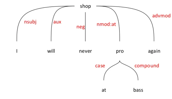
(25) Figure 3.2 shows an example of sentence representation in our method. From a sentence “I will never shop at bass pro again”, after using Stanford Parser, the sentence was represented by: “nsubj(shop-4,i-1) aux(shop-4,will-2) neg(shop-4,never-3) root(ROOT-0,shop-4) case(pro-7,at-5) compound(pro-7,bass-6) nmod:at(shop-4,pro-7) advmod(shop-4,again-8)” We use the tree shown in Figure 3.2 instead of the output of dependency parser for the next step in our model. In this tree, each node is a word, and the edge represents the semantic relation between two words in a sentence.. 3.2. Frequent Sub-tree Mining, Outlier Detection. In this section, we introduce frequent sub-tree mining and how to detect outliers to achieve knowledge from the training set. We also discuss some definitions of frequent sub-tree and how to measure outliers.. 3.2.1. Frequent sub-tree mining. In data mining, frequent sub-tree mining is a problem which determines all subtrees in the database within a minimum support (minsup) threshold. Formally, the definition of sub-tree mining is defined as: Given a threshold minsup, find all trees or sub-trees with support is equal or greater than minsup.. 22.

(26) shop advmod. nsubj. I. aux. will. neg. nmod:at. never. pro case. at. again compound. bass. Figure 3.2: An example about sentence representation by tree. where support is defined as the number of occurrences of a tree or sub-tree in dataset D = {T1 , T2 , ..., Tn } and the support of a tree or sub-tree is defined as:. support(Ti ) =. #Ti |D|. (3.1). where #Ti is the number of advents of tree Ti in dataset D and |D| is total trees in D. A sample dataset is shown in Figure 3.3 which includes two sentences represented by two trees T1 and T2 . With |D| equal to 2 and minsup = 2, all frequent sub-trees are shown in Figure 3.4. While Figure 3.4a, Figure 3.4b and Figure 3.4c are frequent trees with two nodes, Figure ??d, Figure ??e and Figure 3.4f are frequent trees with three nodes and four nodes, respectively.. 23.

(27) shop shop aux. nsubj. neg. nmod:at. neg advmod. I will. aux. advmod. never. will. never. pro case. again. at a) T1. again compound. bass. b) T2. Figure 3.3: The sample dataset of frequent sub-tree mining.. 3.2.2. Outlier detection. Recently, a lot of methods for detecting outliers from datasets have been invented and developed. In this paper, we propose an efficient method for recognising outliers based on frequent sub-tree mining. Although the idea is quite simple, the elimination of outliers in our model makes a significant improvement in the performance of the SC. The frequent sub-tree is well-known as “common pattern” or “common feature” in the dataset. Meanwhile, the others in the dataset were defined as outliers. In the dataset, the outliers have a very small ratio of all data. In this model, OM was defined as a measure to explore the object in outlier set from data. OM of a tree or sub-tree Ti was defined as:. OM (Ti ) =. #Ti − minsup |D|. 24. (3.2).

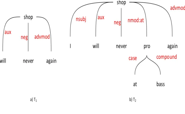
(28) shop. shop. shop aux. neg. nsubj. shop. neg. advmod. will. never. again. a). b). c). will. never d). shop. shop aux. advmod. neg. never. again. will. e). neg. never. advmod. again. f). Figure 3.4: The frequent sub-trees of dataset in Figure 3.3 with minsup = 2. If OM of a tree or sub-tree Ti is negative, Ti belongs to outliers set. After outlier detection phase, from the tree data, we keep a tree or a sub-tree coinciding with the frequent set. Next, we remove all elements with OM < 0 for LSTM + GRNN model in SC problem. From a tree, we will keep or eliminate sub-trees or nodes from the tree. The procedure is shown in Table 3.1. In the FindBestSub-tree procedure table, given a dataset D, minsup, a frequent tree set (FP) and a tree (T), we define the best sub-tree as a tree with eliminating outliers. The elimination is based on frequent set and OM that we described in FindBestSub-tree algorithm. Figure 3.5 shows two trees after removing outliers with two minimum support value. In Figure 3.5a, the tree has five nodes with minsup = 10. With increasing of minsup to 20 from 10 in Figure 3.5b, the tree has four nodes with “again” node in Figure 3.5a.. 25.

(29) Table 3.1: FindBestSub-tree algorithm Algorithm: FindBestSub-tree Input:. T // a tree need to eliminate bad feature D // tree database minsup // minimum support FP //frequent tree set. Output: A sub-tree or A tree 01 Begin 02. If T in FP do. 03 04. return T Else do. 05. Foreach node t in T do. 06. If (OM(t,D,minsup) < 0. 07. eliminate(t). 08. Endif. 09. Endforeach. 10. Endif. 11 End. 26.

(30) shop. I. will. shop. never. again. I. a) minsup = 10. will. never. b) minsup = 20. Figure 3.5: An example of applying FindBestSub-tree algorithm.. 3.3. Representing Frequent Tree or Frequent Subtree. As the previous discussion, a sentence is represented as a tree. For our model, we have to represent the best sub-tree from the previous section by a string of words while keeping relations between parent nodes and child nodes. To capture these relations, we propose a method based on DFS (Depth First Search). We want to represent a tree with relations between parent nodes and child nodes from root to leave nodes. For instance, trees shown in Figure 3.5a and 3.5b were illustrated as “shop I will never again” and “shop I will never”. 3.4. LSTM + GRNN. In this part, we used LSTM + GRNN for training and testing. The main idea of LSTM + GRNN is shown in Figure 3.6 from [22]. Each vector of 200 dimensions represents a word in a sentence, and all words in a sentence are composed of sentence 27.

(31) composition. Next, LSTM represents the vector from composition phase to create a sentence vector in sentence representation phase. All sentence vectors in a document will be evaluated by GRNN to represent as a document vector. Finally, from a document vector, the softmax layer will convert the document vector to conditional probability which is evaluated as follow. exp(xi ) Pi = PC i0 =1 exp(xi0 ) where C is the total of classes in the output.. 28. (3.3).

(32) Softmax. Document Representation. GNN. GNN. GNN. .... Sentence Representation. Word Representation. LSTM. LSTM. .... LSTM. Sentence Composition. Sentence Composition. .... Sentence Composition. .... w1. w2. .... wm. w1. s1. w2. s2. w1. wm .... Figure 3.6: LSTM+GRNN model [22].. 29. .... ... w2. sn. wm.

(33) Chapter 4 Evaluation In this chapter, the evaluation of our model is compared with LSTM + GRNN model. Firstly, we show the information and characteristic of the Multi-Domain dataset. Next, the measures of sentiment classification which is used in this thesis are illustrated in details. Then, the experiment settings and results are described in the experiment settings and results section. Finally, we analyse our experimental results.. 4.1. Corpus. In this thesis, we use the Multi-Domain dataset and Yelp 2013 dataset to evaluate the performance of our model. From Multi-Domain Dataset, we used The Natural Language Toolkit (NLTK)1 for tokenization and splitting the review text to sentences on all dataset. Then, we used the 10-fold cross validation for training and testing. Meanwhile, we use train file and test file of Yelp 2013 from the site of the author of LSTM+GRNN model. The characteristic of both Multi-Domain dataset and Yelp 2013 dataset is shown in Table 4.1.. 4.1.1. Multi-Domain dataset.. The dataset contains four types of product reviews from Amazon: Electronics, Kitchen appliances, Books and DVDs. In each type of product, the dataset includes three files: “positive.review”, “negative.review” and “unlabelled.review”, so we divided all datasets into two categories: 1. http://www.nltk.org/. 30.

(34) • Data 1: include “positive.review” and “negative.review” file. • Data 2: include “unlabelled.review” Each review is rated from 1 to 5 stars, and the author eliminated the reviews with three stars because of the confusion of these reviews. We divided Data 1 and Data 2 with two labels and four labels, respectively. • 4 labels: The labels are review rating. • 2 labels: The labels are positive if its ratings are greater than 3. On the contrary, the labels are negative.. 4.1.2. Yelp 2013 dataset.. This is review dataset from Yelp Dataset Challenge in 2013. The rating star is considered gold label. The author split Yelp 2013 dataset into training, development and testing sets with the 8:1:1 ratio.. 4.2. Evaluation Methods. In this section, we discuss two main measures in sentiment classification, which are used in our model and LSTM + GRNN model. The accuracy and mean square error evaluation method are shown below.. 4.2.1. Accuracy evaluation. Accuracy2 is standard metric to evaluate the performance in sentiment classification and has two definitions: • More commonly, it is a description of systematic errors, a measure of statistical bias; 2. https://en.wikipedia.org/wiki/Accuracy and precision. 31.

(35) 32. 2,000 2,000 2,000 2,000 2,000 2,085 34,743 13,153 16,785 2,085 34,743 13,153 16,785. Kitchens Books DVDs Electronics Kitchens Books DVDs Electronics Kitchens Books DVDs Electronics Kitchens. 33,504. 2,000. Electronics. Yelp 2013 Test. 2,000. DVDs. 268,013. 2,000. Books. Yelp 2013 Train. Data 2. Data 1. #doc. Dataset. 8.87. 8.90. 6.17. 6.96. 9.69. 6.48. 6.17. 6.96. 9.69. 6.48. 6.18. 7.05. 9.42. 9.32. 6.18. 7.05. 9.42. 9.32. #s/d. 159.46. 160.57. 102.7. 121.42. 193.57. 171.68. 102.7. 121.42. 193.57. 171.68. 102.52. 121.61. 183.72. 189.7. 102.52. 121.61. 183.72. 189.7. #w/d. 58,959. 185,069. 68600. 74,410. 74410. 38,539. 68600. 74,410. 74410. 38,539. 19,195. 23,250. 44,185. 44,374. 19,195. 23,250. 44,185. 44,374. |V |. 5. 5. 4. 4. 4. 4. 2. 2. 2. 2. 4. 4. 4. 4. 2. 2. 2. 2. #class. 0.09/0.09/0.14/0.33/0.36. 0.09/0.09/0.14/0.33/0.36. 0.12/0.06/0.19/0.63. 0.15/0.07/0.25/0.53. 0.07/0.05/0.25/0.63. 0.08/0.05/0.23/0.64. 0.18/0.82. 0.21/0.79. 0.12/0.88. 0.13/0.87. 0.33/0.17/0.16/0.34. 0.333/0.167/0.16/0.34. 0.26/0.24/0.14/0.36. 0.27/0.23/0.13/0.37. 0.5/0.5. 0.5/0.5. 0.5/0.5. 0.5/0.5. Class Distribution. Table 4.1: Characteristic of the experimental datasets.

(36) • Alternatively, the ISO defines accuracy as describing both types of observational error above (preferring the term trueness for the common definition of accuracy). And accuracy is defined as:. Accuracy(ACC) =. #correct predictions #total data points. (4.1). where correct prediction is the number of the predictions which are similar with the target outputs, and total data points is the number of all outputs. Assume that the test dataset has 400 instances, and the correct predictions are 350 instances. The accuracy, in this case, look like as. Accuracy(ACC) =. 4.2.2. 350 = 87.5 400. (4.2). Mean Square Error (MSE) evaluation. We used MSE to measure the divergences between predicted label and goal label because one star means strong negative and five star means strong positive. So MSE is defined as PN Accuracy(ACC) =. i=1 (goal. − predicted)2 N. (4.3). where N is the number of all instances in the test dataset; the goal is the label in the test dataset, and predicted is the label from predicting of our model.. 4.3. Experiment Settings. Following LSTM + GRNN model, the settings for the experiment as follow 33.

(37) Implementation settings: • Embedding Length: 200 dimensions • WindowSizeWordLookup1: 1 • WindowSizeWordLookup2: 2 • WindowSizeWordLookup3: 3 • Output Length Word Lookup: 50 • The number of round: 100 • Probability threshold: 0.001 • Learning rate: 0.03 • Randomize base: -0.01 • 10-fold cross validation with 90% training set and 10% testing set Additionally, with Multi-Domain dataset, sub-tree mining was run with several minsup such as 5, 10, 15 and 20. However, in Data 2, minimum support with five was only run in Books dataset because the sub-tree set was very huge, and the average of the number of frequent sub-tree in 10-fold with minsup was shown in Table 4.2. For Yelp 2013 dataset, the minimum support is set as 10, 15, 20, 25, 30, and the average of the number of frequent sub-tree in 10-fold with minsup was shown in Table 4.3. 4.4. Results. Following the previous section, we have the results with LSTM+GRMM and our model with any minimum supports in Table 4.4. From Table 4.4 and Table 4.5, the results have shown that our model achieved high performance with these datasets. The improvements in term of accuracy are ranged of 0.14% - 6.93% over LSTM + GRNN model. 34.

(38) Table 4.2: The average number of frequent sub-tree in 10-fold with minimum support - Multi-Domain dataset. Dataset #class Books 2 DVDs 2 Electronics 2 Kitchens 2 Data 1 Books 4 DVDs 4 Electronics 4 Kitchens 4 Books 2 DVDs 2 Electronics 2 Kitchens 2 Data 2 Books 4 DVDs 4 Electronics 4 Kitchens 4. 4.5. Minsup 5 10 15 20 9,067.7 3284 1855.1 1386.4 8,947.6 3246.1 1866.3 1294.8 6,469.4 2470.5 1488.9 1085.5 5,513.1 2115.6 1262.7 890.8 4,243.6 1523.7 890.7 611.7 3,856 1399.6 799.8 578.7 4,243.6 1523.7 890.7 611.7 2,514.8 1020.3 650.9 475.1 11,675.5 4619.3 2817.5 1953.3 111796.6 97726.4 83350.3 260804.6 123257.5 61219.4 24180.5 14281.1 10018.3 898.8 341.4 211.8 146.1 3441.8 2091.9 1516.2 7454.9 4248.7 2951.7 3822.7 2303.2 1641.2. Results Analysis. Table 4.4 shows an significant improvement of our model than LSTM + GRNN model from 0.14% to 6.93% in Multi-Domain dataset. Overall, our model illustrates high performance in sentiment classification problem. All datasets in Data 1 are data with 2000 documents per dataset so the cost for running frequent mining is acceptable. Hence, we conduct this dataset with minsup = 5, 10, 15 and 20. Most of the results are the best with minsup = 5. At minsup = 5, the number of frequent in Table 4.2 is more than the other minsup so the huge outliers are rejected. Notably, DVDs dataset with two labels is improved by 3.94% from 73.25% to 77.19%. The rule with the efficient results in small minsup is not correctly in Data 2. For example, considering the Data 1, only Books dataset peaked at 77.34% with 35.

(39) Table 4.3: The average number of frequent sub-tree in 10-fold with minimum support - Yelp 2013 dataset. Yelp2013. Minsup 10 15 20 25 30 240,964 163,892 137,141 124,876 99,293. minsup = 10. However, Books, DVDs with two labels and Books with four labels are maximum at minsup = 20. To illuminate the difference, we can see the characteristic of the dataset.As can be seen, the data 2 is larger than Data 1. For instance, while the size of DVDs in Data 2 is about 34,000 documents, the number of documents in Data 1 with DVDs is 2000 documents. Additionally, the class distribution in Data 1 is balance with 50% negative and 50% positive. Meanwhile, the imbalance is shown in the class distribution in Data 2. For example, in Data 2, DVDs is imbalanced with 12% negative and 88% positive. Therefore, Books dataset with four labels in Data 2, for instance, shows high performance, which is increased dramatically by 6.93% from 65.83% to 72.76%. With Yelp 2013 dataset, the results is shown in Table 4.5. Similarly, the results peaked at minsup = 20 by 63.74. 4.6. Error Analysis. Table 4.6 shows some examples in sentiment classification between our model and LSTM+GRNN model, which are correct in our model and did not correct in LSTM+GRNN model. Clearly, the content of these documents is complexity, which mentions about the polarity of the customers on Amazon website. The second column and the fourth of the table 4.6 are the content of documents in original test and our test after removing noises in our model, respectively. The third column and the fifth are the gold rating of LSTM+GRNN mode and Our model, which is positive or negative in the review. The last column is the goal of prediction. In some examples in Table 4.6, two inputs for LSTM+GRNN model in sentiment classification task. With the second and fourth column, the order and the number of the words in sentences are different. Our model changes the original order of words to another order which based on DFS after removing noises in the dataset. These documents from one to six are predicted exactly in our model, which LSTM+GRNN are given incorrect answers. Clearly, documents from one to three are the positive reviews. On the contrary, the negative reviews are documents from four to six in the Table 4.6. For example, in document four, the word ”Do not 36.

(40) 37. Data 2. Data 1. Our model minsup= 10. Our model minsup=5. minsup= 15. Our model. minsup= 20. Our model. 4 2 2 2 2 4 4 4 4. Kitchens. Books. DVDs. Electronics. Kitchens. Books. DVDs. Electronics. Kitchens. 4. Books. 4. 2. Kitchens. Electronics. 2. Electronics. 4. 2. DVDs. DVDs. 2. 73.29. 66.73. 72.95%. 65.83. 92.10. 89.60. 93.48. 87.76. 62.58. 60.63. 50.80. 52.63. 83.64. 81.09. 73.25. 74.29. 0.6674. 0.8354. 0.5469. 1.0645. 0.079. 0.104. 0.0652. 0.1224. 1.314. 1.3077. 1.84. 1.7473. 0.1636. 0.1891. 0.2675. 0.2571. -. -. -. 65.81. -. -. -. 87.95. 62.83. 61.37. 53.48. 53.00. 83.89. 81.45. 77.19. 76.44. -. -. -. 1.0569. -. -. -. 0.1205. 1.2401. 1.4211. 1.5997. 1.7986. 0.1611. 0.1855. 0.2281. 0.2356. 73.43. 67.38. 73.23. 65.67. 92.24. 89.99. 93.78. 87.95. 61.93. 57.93. 53.26. 52.25. 82.04. 77.91. 76.94. 77.34. 0.6358. 0.7999. 0.5266. 1.0803. 0.0776. 0.1001. 0.0622. 0.1205. 1.4276. 1.4947. 1.6872. 1.8399. 0.1796. 0.2209. 0.2306. 0.2266. 73.13. 67.36. 73.08. 66.13. 91.88. 89.62. 93.78. 88.05. 59.64. 57.61. 51.15. 52.08. 81.58. 74.91. 75.73. 74.71. 0.6459. 0.8112. 0.5394. 1.0487. 0.0812. 0.1038. 0.0622. 0.1195. 1.6615. 1.4895. 1.8514. 1.874. 0.1842. 0.2509. 0.2427. 0.2529. 73.11. 66.92. 73.01. 72.76. 91.95. 89.65. 93.79. 88.09. 59.54. 55.75. 49.83. 50.17. 80.07. 72.21. 75.62. 74.36. 0.5403. 0.8. 0.6771. 0.5594. 0.0805. 0.1035. 0.0621. 0.1191. 1.7153. 1.6351. 1.918. 1.9663. 0.1993. 0.2779. 0.2438. 0.2564. #class Acc. (%) MSE Acc. (%) MSE Acc. (%) MSE Acc. (%) MSE Acc. (%) MSE. Books. Dataset. LSTM+GRNN. Table 4.4: Sentiment classification on Multi Domain Dataset. The best results are in bold. Acc is accuracy, and MSE is mean squared error..

(41) Table 4.5: Sentiment classification on Yelp 2013 Dataset. The best results are in bold. Acc is accuracy, and MSE is mean squared error. Yelp2013 Acc(%). MSE. 63.47. 0.5728. minsup =10. 63.49. 0.5661. minsup =15. 63.45. 0.5779. LSTM+GRNN Our model. minsup =20. 63.74 0.5444. minsup =25. 63.45. 0.5779. minsup =30. 63.52. 0.5697. buy” is easy to determine this review is negative because the product is failed to satisfy the review. In document seven to nine, while these are predicted exactly with LSTM+GRNN model, our model predicted incorrectly.. 38.

(42) Table 4.6: Some examples in sentiment classification between our model and LSTM+GRNN model. Doc is Document. Doc. LSTM+GRNN. Label1. Our model. Label2. Goal. 1. If you’re interested in reproducing negative find interested If you ’re positive positive authentic costumes, you won’t find in you wo n’t guide a a better guide to hats and bonnets better to and book than than this book ... this .... 2. I really enjoyed this book .... 3. I can recite most of it from memory, negative love I can most it of positive positive I love it so!... memory from I it so.... 4. ...Do not buy this book unless it is positive ...buy Do not book this negative negative for a middle school student... student unless it is for a middle school .... 5. ...The story just could not keep my positive ...keep story The just negative negative interest. <sssss> I felt no real affincould not interest my ity to any of the characters... <sssss> felt I no real any to characters of the.... 6. ...A friend recommended this book positive ...recommended friend negative negative which I unfortunately bought... A book this bought which I unfortunately.... 7. My order arrived quickly and for a positive order My quickly and negative positive used book it was in excellent shape, book for a used it was looking like new. <sssss> I won’t in excellent looking new hesitate to order from this company like <sssss> I wo n’t again... order to company from this again.... 8. I haven’t had a chance to read the positive had I have n’t chance a negative positive book in its entirity, but have enjoyed read to book the in its what I have read. but enjoyed have read what I have. 9. Sorry for the sarcastic title ... negative Sorry title for the ... positive negative <sssss> If you are into reading re<sssss> sure reading If lationship books, just be sure this you are into books reisn’t your only resource. lationship just be resource this is n’t your only. negative enjoyed I really book positive positive this.... 39.

(43) Chapter 5 Conclusions and Future Work 5.1. Conclutions. A method for SC with the combination of dependency parser, sub-tree mining, and deep learning was proposed in this paper. This approach encodes the relation among words by the dependency tree and some features in a sentence are rejected by sub-tree mining and FindBestSub-tree algorithm in outlier detection phase. For validating the efficiency of the proposed model, experiments were conducted on Multi-Domain Dataset, which is a popular dataset in SC. The results have shown that the proposed method is superior to using only LSTM + GRNN model. However, when the minimum support value is very low, the cost of running sub-tree is very high because the vast number of candidates are generated. This thesis presented our model that is an approach to sentiment classification problem. We use some technique in NLP to representing the semantic relation in a sentence and LSTM + GRNN in the document. In the current research, we only use dependency parser to extract relation information among works in a sentence. The advantage of our model is easy to understand and implement with high performance. The drawback also exists in representing the semantic relation among siblings node due to DFS representing a tree by a string of words. Another limitation of our model is the illustration by dependency parser because the parser is based on grammar structure.. 40.

(44) 5.2. Future Work. Since the cost of sub-tree mining and FindBestSub-tree is huge, we will study to look for the solutions for outlier detection and continuously find the method for capturing relation words in a sentence from dependency trees. Additionally, we also expand our work to get minsup automatically and sentiment-sensitive discourse relations such as “condition”, “cause”, “contrast”, etc. We will expand how to represent semantic relations in among words and sentences by the semantic graph. The semantic graph includes a lot of information about the context of the text through the link in the graph. From the information, we extract and select efficient features for sentiment analysis problem. Another future work is that we will construct a deep learning model to capture semantic relations from the semantic graph to capture automatically.. 41.

(45) Bibliography [1] Kenji Abe, Shinji Kawasoe, Tatsuya Asai, Hiroki Arimura, and Setsuo Arikawa. Optimized substructure discovery for semi-structured data. In Principles of Data Mining and Knowledge Discovery, pages 1–14. Springer, 2002. [2] Kenji Abe, Shinji Kawasoe, Tatsuya Asai, Hiroki Arimura, and Setsuo Arikawa. Principles of Data Mining and Knowledge Discovery: 6th European Conference, PKDD 2002 Helsinki, Finland, August 19–23, 2002 Proceedings, chapter Optimized Substructure Discovery for Semi-structured Data, pages 1–14. Springer Berlin Heidelberg, Berlin, Heidelberg, 2002. [3] Apoorv Agarwal, Boyi Xie, Ilia Vovsha, Owen Rambow, and Rebecca Passonneau. Sentiment analysis of twitter data. In Proceedings of the workshop on languages in social media, pages 30–38. Association for Computational Linguistics, 2011. [4] Markus M Breunig, Hans-Peter Kriegel, Raymond T Ng, and J¨org Sander. Lof: identifying density-based local outliers. In ACM sigmod record, volume 29, pages 93–104. ACM, 2000. [5] Yun Chi, Richard R. Muntz, Siegfried Nijssen, and Joost N. Kok. Frequent subtree mining - an overview. Fundam. Inf., 66(1-2):161–198, November 2004. [6] Gayatree Ganu, Noemie Elhadad, and Am´elie Marian. Beyond the stars: Improving rating predictions using review text content. In WebDB, volume 9, pages 1–6. Citeseer, 2009. [7] Andrew B Goldberg and Xiaojin Zhu. Seeing stars when there aren’t many stars: graph-based semi-supervised learning for sentiment categorization. In Proceedings of the First Workshop on Graph Based Methods for Natural Language Processing, pages 45–52. Association for Computational Linguistics, 2006.. 42.

(46) [8] Zengyou He, Xiaofei Xu, Joshua Zhexue Huang, and Shengchun Deng. Advances in Web-Age Information Management: 5th International Conference, WAIM 2004, Dalian, China, July 15-17, 2004, chapter A Frequent Pattern Discovery Method for Outlier Detection, pages 726–732. Springer Berlin Heidelberg, Berlin, Heidelberg, 2004. [9] Zengyou He, Xiaofei Xu, Joshua Zhexue Huang, and Shengchun Deng. A frequent pattern discovery method for outlier detection. In Advances in Web-Age Information Management, pages 726–732. Springer, 2004. [10] Yoon Kim. Convolutional neural networks for sentence classification. arXiv preprint arXiv:1408.5882, 2014. [11] Edwin M Knox and Raymond T Ng. Algorithms for mining distancebased outliers in large datasets. In Proceedings of the International Conference on Very Large Data Bases, pages 392–403. Citeseer, 1998. [12] Taku Kudo, Jun Suzuki, and Hideki Isozaki. Boosting-based parse reranking with subtree features. In Proceedings of the 43rd Annual Meeting on Association for Computational Linguistics, pages 189–196. Association for Computational Linguistics, 2005. [13] Jiwei Li, Dan Jurafsky, and Eudard Hovy. When are tree structures necessary for deep learning of representations? arXiv preprint arXiv:1503.00185, 2015. [14] James Martens and Ilya Sutskever. Learning recurrent neural networks with hessian-free optimization. In Proceedings of the 28th International Conference on Machine Learning (ICML-11), pages 1033–1040, 2011. [15] Bo Pang and Lillian Lee. Seeing stars: Exploiting class relationships for sentiment categorization with respect to rating scales. In Proceedings of the 43rd Annual Meeting on Association for Computational Linguistics, pages 115–124. Association for Computational Linguistics, 2005. [16] Bo Pang, Lillian Lee, and Shivakumar Vaithyanathan. Thumbs up?: sentiment classification using machine learning techniques. In Proceedings of the ACL02 conference on Empirical methods in natural language processing-Volume 10, pages 79–86. Association for Computational Linguistics, 2002. [17] Lizhen Qu, Georgiana Ifrim, and Gerhard Weikum. The bag-of-opinions method for review rating prediction from sparse text patterns. In Proceedings of the 43.

(47) 23rd International Conference on Computational Linguistics, pages 913–921. Association for Computational Linguistics, 2010. [18] Sridhar Ramaswamy, Rajeev Rastogi, and Kyuseok Shim. Efficient algorithms for mining outliers from large data sets. In ACM SIGMOD Record, volume 29, pages 427–438. ACM, 2000. [19] Mo Shen, Daisuke Kawahara, and Sadao Kurohashi. Dependency parse reranking with rich subtree features. Audio, Speech, and Language Processing, IEEE/ACM Transactions on, 22(7):1208–1218, 2014. [20] Richard Socher, Alex Perelygin, Jean Y Wu, Jason Chuang, Christopher D Manning, Andrew Y Ng, and Christopher Potts. Recursive deep models for semantic compositionality over a sentiment treebank. In Proceedings of the conference on empirical methods in natural language processing (EMNLP), volume 1631, page 1642. Citeseer, 2013. [21] Songbo Tan and Jin Zhang. An empirical study of sentiment analysis for chinese documents. Expert Systems with Applications, 34(4):2622–2629, 2008. [22] Duyu Tang, Bing Qin, and Ting Liu. Document modeling with gated recurrent neural network for sentiment classification. In Proceedings of the 2015 Conference on Empirical Methods in Natural Language Processing, pages 1422–1432, Lisbon, Portugal, September 2015. Association for Computational Linguistics. [23] Peter D Turney. Thumbs up or thumbs down?: semantic orientation applied to unsupervised classification of reviews. In Proceedings of the 40th annual meeting on association for computational linguistics, pages 417–424. Association for Computational Linguistics, 2002. [24] Sida Wang and Christopher D Manning. Baselines and bigrams: Simple, good sentiment and topic classification. In Proceedings of the 50th Annual Meeting of the Association for Computational Linguistics: Short Papers-Volume 2, pages 90–94. Association for Computational Linguistics, 2012. [25] Mohammed J Zaki. Efficiently mining frequent trees in a forest. In Proceedings of the eighth ACM SIGKDD international conference on Knowledge discovery and data mining, pages 71–80. ACM, 2002. [26] Mohammed J. Zaki. Efficiently mining frequent trees in a forest. In Proceedings of the Eighth ACM SIGKDD International Conference on Knowledge Discovery and Data Mining, KDD ’02, pages 71–80, New York, NY, USA, 2002. ACM. 44.

(48) [27] Shusen Zhou, Qingcai Chen, and Xiaolong Wang. Active deep networks for semi-supervised sentiment classification. In Proceedings of the 23rd International Conference on Computational Linguistics: Posters, pages 1515–1523. Association for Computational Linguistics, 2010.. 45.

(49)