M A C H I N E L E A R N I N G A P P R O A C H E S F O R B I O L O G I C A L A N D P H Y S I O L O G I C A L D ATA
R A I S S A T I L L A D A R E L AT O R
A dissertation submitted in partial fulfillment of the requirements for the degree of Doctor of Philosophy
Division of Electronics and Informatics Graduate School of Science and Technology
Gunma University February 2015
Raissa Tillada Relator: Machine Learning Approaches for Biological and Physiological Data,© February 2015
I don’t know anything,
but I do know that everything is interesting if you go into it deeply enough.
— Richard Feynman
Para kay nanay at tatay.
A B S T R A C T
Machine learning has proven itself to be a powerful tool in different tasks such as classification, pattern recognition, and data mining and analysis. However, with the increasing amount of available information, different structures and nature of data require different approaches for data utilization to warrant optimal results.
With the aim to exploit biological and physiological data used in recently trending fields such as bioinformatics, chemoinformatics, neuroinformatics and brain-computer interfaces, learning algorithms that can outperform conventional methods in these areas are developed in this thesis.
The first part of this work, which concerns the use of biological data, focuses on predicting interactions between drugs and proteins, and finding active sites in enzymes. For the first task, a variant of canonical correlation analysis is introduced and utilized to improve the performance of learning machines in predicting drug-protein interactions, where the approach is derived from the generalized eigenvalue problem. As for the latter, a learning algorithm exploiting Bregman divergences is developed to determine a weighting scheme to be used in the computation of the deviation in finding active sites in enzymes.
The second part, which addresses physiological data, focuses on task classification using EEG signals. The data signals can usually be modeled as a vector sequence or set of vectors. For this type of input in classification tasks, a kernel function is proposed. This thesis also presents a link between the said kernel function and an existing Grassmann kernel.
The performances of all methods proposed in this work are investigated using real-world data. Empirical results show the efficiency and potential advantages of the proposed algorithms over conventional methods.
v
A C K N O W L E D G M E N T S
First and foremost, I would like to give my sincerest gratitude to my supervisor, Professor Tsuyoshi Kato, for all his support and patience as my mentor, as well as my guardian in a foreign land away from home. His efforts and advices have made me a better student, researcher, and individual. This thesis would not have been possible without his supervision.
I am also grateful to Professor Yoichi Seki, Professor Hidetoshi Yokoo, Professor Naohya Ohta, and Professor Yoshikuni Onozato for agreeing to serve on my committee, and setting aside some time off their very busy schedule to review this thesis.
I am thankful to past and present members of Kato Laboratory, especially to Eisuke Ito and Yoshihiro Hirohashi for their inputs and assistance in my researchh. I also appreciate the researchers I had the opportunity to collaborate with. I would like to give due thanks to all my professors in Gunma University for their guidance and for imparting their knowledge. Likewise, I would like to acknowledge the people from the Student Support Section and department office who have been so kind and accommodating all throughout my stay in the university.
I would always be grateful for friends I have made here in Japan, some of whom have been like family to me. Special mention goes to Meerin and Ou, who have been dear friends even in tough times. To my teachers and classmates in the language classes, thank you very much for making my stay more interesting and enjoyable. I would also like to extend my thanks to friends back home and abroad, for keeping in touch and for the small messages that bring smiles.
I would like to thank my family for their unending love, support and encouragement. And most of all, to W. There are not enough words to describe how truly grateful I am.Maraming salamat.
Finally, I would like to acknowledge the generous help of the Japanese Ministry of Education, Culture, Sports, Science and Technology for funding my PhD studies.
vii
C O N T E N T S
1 I N T R O D U C T I O N 1 2 P R E L I M I N A R I E S 5
2.1 Notational Conventions 5
2.2 The Binary Classification Problem 5 2.3 Support Vector Machines 6
2.4 Kernel Functions 9
3 P R E D I C T I N G P R O T E I N-L I G A N D I N T E R A C T I O N S 11 3.1 Related works 13
3.2 Methodology 14
3.2.1 Overview of the Algorithm 14 3.2.2 Weighted CCA 17
3.2.3 Weighted SVM 18 3.2.4 Weighting schemes 18 3.3 Experiments and Results 19
3.3.1 Data and Experimental Settings 19 3.3.2 Performance Evaluation Criteria 20 3.3.3 Effects of Using CCA and Weighting 21 3.3.4 Weighted SVM vs Classical SVM 24 3.3.5 Using Interaction Profiles 24
3.4 Summary 25
3.5 Supporting Theories and Proofs 26
3.5.1 Generalized Eigendecomposition 26 3.5.2 Linear Weighted CCA 29
3.5.3 Kernel Weighted CCA 32 3.5.4 Weighted SVM 34
4 E N Z Y M E A C T I V E S I T E P R E D I C T I O N 35 4.1 Active Site Search Method 37
4.2 Learning Algorithm 39
4.2.1 Optimization Algorithm 41 4.3 Experiments and Results 42 4.4 Summary 43
5 C L A S S I F Y I N G TA S K S F R O M E E G S I G N A L S 45 5.1 Preliminaries 47
5.2 Grassmann Kernels and Related Methods 48 5.3 Mean Polynomial Kernel 50
5.4 Mean Polynomial Kernel and Projection Kernel Relationship 51
5.5 Experiments and Results 52
ix
x C O N T E N T S
5.5.1 EEG Signal Task Classification 52 5.5.2 Efficiency Comparison 55
5.5.3 Discussion 56 5.6 Summary 57
5.7 Proofs and Discussion 57
5.7.1 Derivation of Equation (5.3) 57 5.7.2 Derivation of Equation (5.4) 57
5.7.3 Explicit Representation of Features 58 6 C O N C L U S I O N A N D F U T U R E D I R E C T I O N S 59
B I B L I O G R A P H Y 61
L I S T O F F I G U R E S
Figure 2.1 An illustration of the margin. 7 Figure 2.2 An illustration of the kernel trick. 10 Figure 3.1 Protein-ligand matrix and descriptors. 12 Figure 3.2 Illustration of Classical CCA vs Weighted
CCA. 16
Figure 3.3 Average performance of all methods for the task of protein-ligand prediction. 22
Figure 3.4 Histograms illustrating the comparisons between the proposed method WW and other methods. 23
Figure 3.5 ROC curves. 25
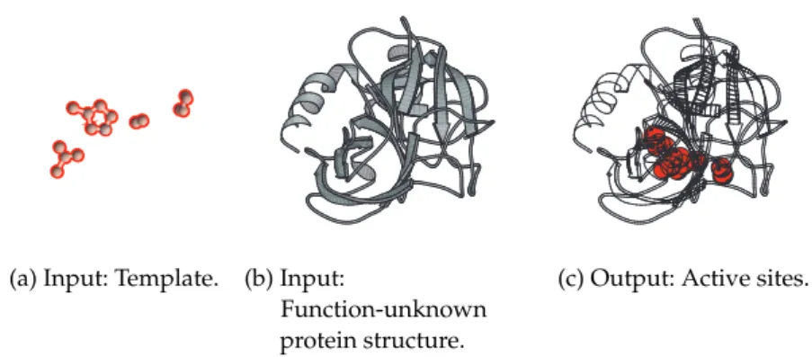
Figure 4.1 The active site search problem. 37
Figure 4.2 Comparison between a local site and a template. 38
Figure 4.3 Dataset for training. 39
Figure 4.4 Average performance of all methods for the task of enzyme active site prediction. 43 Figure 5.1 Sample position map of EEG sensors. 46 Figure 5.2 EEG signals as a sequence of vectors. 46 Figure 5.3 Flow of methodology for computing the kernel
value for the Grassmann kernels and the mean polynomial kernel. 49
Figure 5.4 Average performance of all methods for the EEG signal task classification. 54
Figure 5.5 Cumulative ratio distribution of the eigenvalues as dimensionmis varied. 54
L I S T O F TA B L E S
Table 3.1 Abbreviation of methods. 20
Table 5.1 Time complexity comparison of the kernels. 55
xi
1
I N T R O D U C T I O N
We are currently in the era of “big data.” This data deluge came with the progression of modern technology. With the evolution of the Internet, high tech machineries, advanced medical technologies, and personal computers, a plethora of data of various types is continuously being generated. And there has been a demand to harness these to extract some valuable information that can be used to our advantage.
Machine learning has proven itself to be a powerful tool in different tasks such as classification, pattern recognition, and data mining and analysis [16, 29, 52, 72, 74]. These tasks can further be extended to varying applications such as in biometrics and security, computer vision, data intrusion, drug design, medical imaging, and social data analysis. However, with the increasing amount of available information, different structures and nature of data require different approaches for data utilization to warrant optimal results. Hence, there is a need to continuously challenge the conventional methods.
Machine learning algorithms can be divided into 3 types:
supervised, unsupervised, and reinforcement learning. Supervised learning makes use of a part of the whole data for training to allow the algorithm to “learn” some mapping that can perform predictions.
Here, the presence of the training data set allows us to measure the performance of the algorithm by defining error metrics, such as the difference between the predicted values and the true values.
On the other hand, in the unsupervised approach, the goal is usually to find some noteworthy patterns that can be utilized for data analysis.
Thus, this is also sometimes referred to as knowledge discovery [52].
Unlike in supervised learning, the type of patterns that are expected to be uncovered are not explicitly known, neither can any error metric be defined. Examples of this type include clustering, hidden Markov models, and computational methods such as principal component analysis and singular value decomposition, among others.
Reinforcement learning may be the less commonly used type compared to the previous two. This form of learning is inspired by behavioral psychology, where reward and punishment are usually given to teach subjects how to act. By doing this, the subject is trained on which tasks he/she is encouraged to perform, and which are not.
Thus, this also arises in areas such as control theory and robotics.
In this work, however, we will only focus on supervised learning.
In particular, we are interested in binary classification tasks where training data are utilized to approximate some relationship between
1
2 I N T R O D U C T I O N
input and output variables, which can further be used to categorize new inputs into one of two classes.
T H E S I S O R G A N I Z AT I O N A N D C O N T R I B U T I O N S
The studies involved in this thesis contribute to the improvement of machine learning methods for binary classification problems.
In particular, we focus our works on bioinformatics- and brain- computer interface-related themes. Following a short introduction of the binary classification problem, support vector machines (SVMs) and kernel methods, and some notations introduced in Chapter2, the contributions of this thesis are divided and summarized accordingly:
• In Chapter 3, we present a variant of canonical correlation analysis and use this to improve the performance of learning machines in predicting interactions between ligands/drugs and proteins. Protein-ligand interaction prediction plays an important role in drug design and discovery. However, wet lab procedures are inherently time consuming and expensive due to the vast number of candidate compounds and target genes.
Hence, computational approaches became imperative and have become popular due to their promising results and practicality.
Such methods require high accuracy and precision outputs for them to be useful, thus, the problem of devising such an algorithm remain very challenging. In this chapter, we propose an algorithm employing both support vector machines and an extension of canonical correlation analysis (CCA). Following assumptions of recent chemogenomic approaches, we explore the effects of incorporating bias on similarity of compounds.
We introduce kernel weighted CCA as a means of uncovering any underlying relationship between similarity of ligands and known ligands of target proteins.
• In the succeeding Chapter4, we exploit some Bregman distances to develop a learning algorithm that automatically determines the weights for atoms in finding active sites in enzymes.
Prediction of active sites in enzyme is very important for the study of proteins and for practical applications such as drug design. Underlying mechanisms for enzyme reaction are based on the local structures of their active sites. Because of this, the mean square deviation has often been used for protein local structure comparison. To improve the ability of such simple measure, various types of template-based methods that compare local sites have been developed to date. In this work, we introduce parameters for the deviation, as well as regularization functions using Bregman divergences to model a new machine
I N T R O D U C T I O N 3
learning algorithm that determines the parameters of the square deviation.
• In Chapter 5, we propose a kernel function for data modeled as vector sequences or sets of vectors, such as physiological data like electroencephalography (EEG) signals. Classification tasks in brain-computer interface research have presented several applications, biometrics and cognitive training, for instance. However, like in any other discipline, determining suitable representation of data has been challenging, and recent approaches have deviated from the familiar form of one vector for each data sample. In this chapter, we consider a kernel between vector sets, motivated by recent studies where data are approximated by linear subspaces, in particular, methods that were formulated on Grassmann manifolds. The kernel takes a more general approach given that it can also support input data that can be modeled as a vector sequence, and not necessarily requiring it to be a linear subspace. We also discuss how the kernel can be associated with the Projection kernel, a known Grassmann kernel.
Finally, Chapter6concludes our work with a summary and discussion of future works related to the proposed methods.
P U B L I S H E D R E S U LT S
The works contained in this thesis have resulted in 2 journal publications in the Information Processing Society of Japan (IPSJ) Transactions on Bioinformatics [61], and in the Institute of Electronics, Information and Communication Engineers (IEICE) Transactions on Information and Systems [62]. The contents have also been disseminated at relevant conferences and SIG meetings, where a total of 5 articles have been accepted for presentation [63,64,65,66,67].
2
P R E L I M I N A R I E S
In this chapter we introduce the basic notations and briefly review some mathematical concepts that have been incorporated in this thesis. References [11,16,29,52,72,74] are recommended to readers who wish to have more detailed information about support vector machines, kernel methods, machine learning, and other related subjects.
2.1 N O TAT I O N A L C O N V E N T I O N S
We will useR andN to denote the set of real and natural numbers, RnandNnfor the set ofn-dimensional real and natural vectors, and Rm×n for the set ofm×nreal matrices. The set of nonnegative real numbers is represented byR+, and the set of positive real numbers by R++. For any n ∈ N, we will use Nnto represent the set of natural numbers less than or equal to n. We will denote vectors by bold- faced lower-case letters and matrices by bold-faced upper-case letters.
Entries of vectors and matrices are not bold-faced. The transpose of a matrixMis given byMT, the inverse isM−1, while then×nidentity matrix is In. The n-dimensional vector whose entries are all one is denoted by1n, while0nis then×1vector of all zeros. The operation diag(M) outputs a vector whose entries are the diagonal entries of matrixM, while diag(v)returns the diagonal matrix with the entries of vectorvalong the diagonal. We will useSnto denote the set ofn×n symmetric matrices, andOm×nthe set ofm×northonormal matrices, i.e.Om×n ≡ {M ∈ Rm×n|MTM = In}. This definition implies that Om×n = ∅ if m < n. For simplicity, we shall also assume that the input spaceXis a Euclidean space, i.e.,X⊆Rn.
2.2 T H E B I N A R Y C L A S S I F I C AT I O N P R O B L E M
Before our introduction on support vector machines and kernel methods, we start by formally defining the classification problem in supervised learning.
As previously stated, classification, as supervised learning, aims to learn or approximate a mapping from inputs denoted by x ∈ Rn to outputs represented by y, given some data for training. The input vectorsxare usually calledfeaturesorattributes. And the value of the output variable yis either nominal or categorical, depending on the classification task, which tells us the true class of the input.
5
6 P R E L I M I N A R I E S
In the simplest case whereyis nominal and the number of classes is equal to two, we have y ∈ {±1}. This is referred to as the 2-class or binary classification problem. This may further be extended into N number of classes, or what we call themulti-classificationproblem. In the case wherey∈R, we call itregression. In this work, we will mainly focus on binary classification problems.
To formally define classification problem, suppose we have a set of
`training dataD= {(xi,yi)}`i=1 consisting of input-output pairs. The task is to find an approximatedecision functionf:x7→yusing theD.
2.3 S U P P O R T V E C T O R M A C H I N E S
First introduced in 1992 by V. Vapnik and colleagues from the AT&T Labs, support vector machines (SVMs) are known to have the ability of being universal approximators of any multivariate function much similar to neural networks. Despite their strong theoretical background, SVMs did not receive much attention until publications showing their excellent performance in practical applications such as text categorization, digit recognition and computer vision arise (cf.
[16,72] for some examples).
To address the task of classifying data, Vapnik et al. first considered a class of hyperplanes with equation
hw,xi+b=0,
in some dot product spaceX, wherew∈Xandb∈R, corresponding to the decision function
f(x) =sgn(hw,xi+b). (2.1) The value hw,xi+b is also sometimes referred to as the SVM score, as it also provides a level or degree of confidence in classifying x.
Following this, they then proposed a learning algorithm for linearly separable problems.
2.3 S U P P O R T V E C T O R M A C H I N E S 7
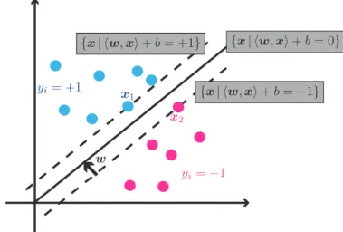
Figure 2.1:An illustration of the margin. Here, the data points on the left belong to the class where y = +1, while the points on the right belong to y = −1. The two classes are separated by the hyperplane with equation hw,xi+b = 0, where w is the vector normal to the hyperplane. Between the dashed lines with equations hw,xi+b = +1 andhw,xi+b = −1, the size of the marginis equal tokwk2 .
In the context of the simple binary classification problem, SVMs use hyperplanes to create classifiers that maximize the margin, such as that in Figure 2.1. By maximizing the margin, classification error is minimized when new data points are introduced. With the classifier being more robust to perturbations in the data, the problem of underfitting or loose classification, and overfitting or tight classification of the data can be avoided. The binary classification problem is then equivalent to the task of finding a hyperplane that separates the data such that the margin of separation between any training point and the hyperplane is a maximum. This can be formulated as
maximize min{kx−xik: x∈X,hw,xi+b=0, i=1,. . .,`}
wrt w∈X, b∈R. (2.2)
A unique solution for this problem exists and is called the optimal hyperplane, also referred to as themaximal margin classifier.
In order to construct the optimal hyperplane, the learning problem for SVMs presented in (2.2) can be rewritten as the constrained quadratic optimization problem
minimize 1 2kwk2
wrt w∈X, b∈R,
subject to yi(hw,xii+b)>1,∀i=1,2,. . .,`, (2.3)
8 P R E L I M I N A R I E S
where w is the normal vector to the hyperplane. To solve this quadratic optimization problem, Lagrange multipliers αi0s are introduced, and the Lagrangian function is given by
L(w,b,α) = 1
2kwk2− X` i=1
αi(yi(hw,xii+b) −1). Hence, problem (2.3) has the primal form
minimize L(w,b,α) = 1
2kwk2− X` i=1
αi(yi(hw,xii+b) −1), wrt w∈X, b∈R,
subject to yi(hw,xii+b)>1,∀i=1,2,. . .,`, and dual form given by
maximize W(α) = X` i=1
αi−1 2
X` i,j=1
αiαjyiyj xi,xj
wrt α∈R`,
subject to αi>0,∀i=1,. . .,`, and X` i=1
αiyi=0.
By minimizing the Lagrangian L with respect to the primal variables w and b, and maximizing it with respect to the dual variables αi0s, we can obtain the saddle point which will lead us to the solution. To do this, the Karush-Kuhn-Tucker (KKT) conditions are imposed. The KKT conditions state that at the saddle point, the partial derivatives with respect to the primal variables must be zero, i.e.,
∂
∂bL(w,b,α) = − X` i=1
αi=0 and
∂
∂wL(w,b,α) = w− X` i=1
αiyixi=0.
And thus we must have X` i=1
αi=0 and w= X` i=1
αiyixi. (2.4) The vectors xj in the solution vector w in Equation (2.4) whose coefficients αj are nonzero are called support vectors. In Figure 2.1, these are the data points x1 and x2, which are points lying on the margin represented by the dashed lines. Finally, using the solution in Equation (2.4) expressed in terms of support vectors, the decision
2.4 K E R N E L F U N C T I O N S 9
function from Equation (2.1) can now be rewritten as thesupport vector classifier
f(x) =sgn X` i=1
αiyihx,xii+b
!
. (2.5)
It can be observed from the form that these classifiers only operate with the inner product. Hence, they can still be very efficient even in high dimensional input spaces.
There are also other variants of SVM such as that using soft-margin, one-class SVM, and support vector regression. However, we will no longer include the vast details of these types of SVM.
2.4 K E R N E L F U N C T I O N S
Kernel methods are a class of pattern recognition algorithms, with their best known element as the support vector machine. Since linear classifiers such as SVM may not work well when data has a more complex pattern, a nonlinear mappingφfrom the original input space Xto some higher dimensional spaceFis often introduced to address this issue. A kernel is then defined as a function K such that for any two data pointsx1,x2in an input spaceX,
K(x1,x2) =hφ(x1),φ(x2)i,
where φ is a mapping from X to an inner product space F called a feature space. Hence, kernel methods are a class of algorithms that perform by mapping the input data into a high dimensional feature space. This is done using the so-called kernel trick which is primarily based on Mercer’s theorem:
Theorem 2.1(Mercer’s Theorem). Any continuous, symmetric, positive semidefinite kernel function K(x,y) can be expressed as a dot product in a high dimensional space.
The theorem implies that any algorithm employing the inner product operation can be applied with the kernel trick. For instance, the binary decision function in (2.5) for the support vector classifier can easily be rewritten as
f(x) =sgn X` i=1
αiyihφ(x),φ(xi)i+b
!
=sgn X` i=1
αiyiK(x,xi) +b
! . The kernel trick is utilized especially in cases when data is not linearly separable. By applying the kernel trick, data is projected in a higher dimensional space F before performing classification. This gives rise to linear classifiers or hyperplanes in the feature space F, and hence creating nonlinear classifiers or hypersurfaces when projected back to the original input space, like in the example in Figure 2.2.
10 P R E L I M I N A R I E S
linear classifier
hyperplane classifier
nonlinear classifier
Figure 2.2:An illustration of the kernel trick.
Indeed, kernel-based algorithms have come a long way since their introduction due to their many advantages and potential. At present, there is an extensive list of kernels used in varying applications and types of data. Among them, the most recognized and widely- used are the linear kernel (k(x1,x2) = hx1,x2i), the polynomial kernel k(x1,x2) = hx1,x2id+c, c ∈ R
, and the Gaussian RBF kernel
k(x1,x2) = exp
− kx12σ−x22k2
, σ > 0
functions. Aside from the fact that kernel functions have provided algorithms a bridge between linearity and nonlinearity, their performance have been proven comparable to, if not better than, existing algorithms in various areas where they have been exploited. Also, applying the kernel trick is very straightforward and new kernels are easy to construct. And lastly, there is less concern given to the dimension of the feature space due to the simple dot product operation that renders the algorithms computationally inexpensive than usual. For these reasons, recent machine learning trends have involved “kernelizing” some already established algorithms.
3
P R E D I C T I N G P R O T E I N - L I G A N D I N T E R A C T I O N S
Drug discovery is a multi-staged process which involves the determination of existing interactions between a compound and a protein. Many drugs are developed depending on the reaction they produce when coupled with the respective proteins acting during a biological process in the body. However, only a few existing interactions have actually been validated through experiments.
Moreover, wet lab procedures are inherently time consuming and expensive due to the vast number of candidate compounds and target genes. Hence, computational approaches became imperative and have become popular due to their promising results and practicality.
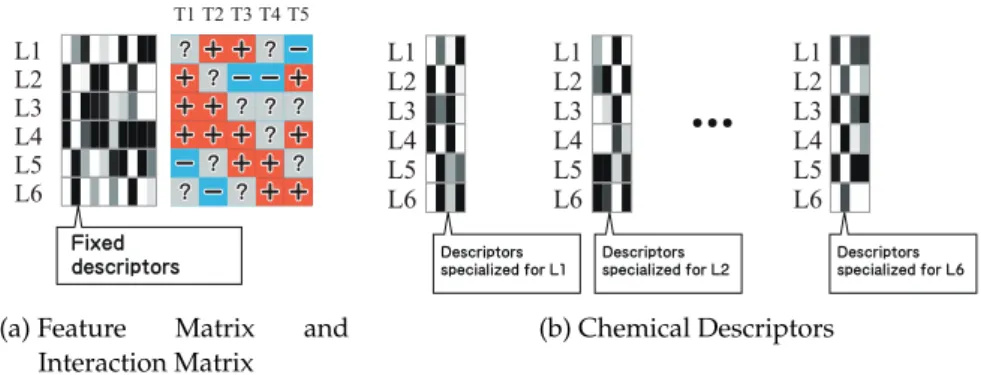
The protein-ligand interaction prediction problem can be viewed as a task of filling up a protein-ligand matrix whose rows represent the candidate compounds and the columns represent the target proteins as shown in the example in Figure 3.1a. A matrix entry is +1 if there is interaction between the corresponding drug and target.
Otherwise,−1. Only a few interactions have actually been verified and recorded which makes the protein-ligand matrix sparse. Termed as the
‘chemogenomic approach’ by Rognan [68], the ultimate goal of this task is to identify all the ligands of each target, thus, fully matching the ligand and target spaces [3].
Many in silico methods have already been developed to address this problem. We can classify these methods into two: the structure or docking approach and the ligand-based approach. Docking approaches make use of 3D structures of the chemical compounds or the proteins to find protein-ligand pairs which are more likely to bind [2, 4, 7]. On the other hand, ligand-based techniques usually employ machine learning algorithms in comparing known ligands and candidate ligands of a certain target even without any prior information regarding their structure [14, 33, 80]. In this study, we shall make use of the ligand-based approach.
There are two ways of approaching the task of interaction prediction: one is by using the global model [2, 56], and another one is via the local model [3, 33, 80]. The global model utilizes a large interaction matrix and imputation of missing values is done simultaneously. Each cell in the interaction matrix is considered as a sample to which statistical methods are applied. Descriptors of ligands in the form of a feature matrix and some information for target proteins are combined to generate a fused profile for each cell in the interaction matrix. An advantage is that interaction prediction for target proteins with few known interactions can still be formed.
However, since the model aims to exploit information from similar
11
12 P R E D I C T I N G P R O T E I N-L I G A N D I N T E R A C T I O N S
L3 L4 L5 L6
T1 T2 T3 T4 T5
L1 L2
ṩ ṩ ṩ ṩ ṩ
ṩ ṩ ṩ ṩ ṩ ṩ ṩ ṩ
ṩ ṩ ṩ
ṰẓẢẏẎ Ẏẏẝẍẜẓẚẞẙẜẝ
(a) Feature Matrix and Interaction Matrix
L3 L4 L5 L6 L1 L2
L3 L4 L5 L6 L1 L2
L3 L4 L5 L6 L1 L2
Ṯẏẝẍẜẓẚẞẙẜẝ ẝẚẏẍẓẋẖẓẤẏẎΏẐẙẜΏṶṛ
Ṯẏẝẍẜẓẚẞẙẜẝ ẝẚẏẍẓẋẖẓẤẏẎΏẐẙẜΏṶṜ
Ṯẏẝẍẜẓẚẞẙẜẝ ẝẚẏẍẓẋẖẓẤẏẎΏẐẙẜΏṶṠ
ṘṘṘ
(b) Chemical Descriptors
Figure 3.1:Protein-ligand matrix and descriptors.In the example depicted in (a), the prediction task is to impute 11 missing entries in the 6×5protein-ligand matrix using10-dimensional raw descriptors of ligands. The problem can be divided into six sub-problems, each of which is to complete a row in the protein-ligand matrix.
Our algorithm extracts compact descriptors specialized in each sub-problem.
columns, some useful information for learning the rule for prediction may be corrupted by information from irrelevant columns.
Meanwhile, in the local model approach, prediction is made for each column of the protein-ligand table independently — the approach finds unknown chemical compounds which are similar to known ligands interacting with the target protein of interest. The local model often suffers from a small-sample problem. Many columns in the protein-ligand interaction matrix include few positive interactions, causing machine learning algorithms to be trained with few positive samples despite very high dimensionality of ligand descriptors.
The goal of determining interactions between targets and compounds is established under twofold assumptions [3, 68]: First is that compounds with similar properties tend to share targets.
And, targets with similar ligands share similarities in structures such as binding sites. These have been verified by recent studies by considering drug side effects [12] and similarities among ligands [51]. Moreover, integrated approaches exploring both protein and compound similarities have also been investigated [10, 33, 85].
Thus, recent methodologies have allowed us to make predictions on interactions based on similarity measures for ligands and targets.
Motivated by the assumption that similar ligands tend to have similar target proteins [42,73], our goal is to uncover any underlying relationship between a set of ligands and exploit this relationship, together with some known ligand-target interactions, to predict new interactions. We search for ligands with strong associations by finding correlations between them using their features.
In this chapter, we present a weighted extension of canonical correlation analysis (WCCA) in the reproducing kernel Hilbert space
3.1 R E L AT E D W O R K S 13
(RKHS) in an attempt to introduce advantageous properties of local models to the global model approach. To estimate the missing entries in each row of the interaction matrix, we use kernel WCCA (KWCCA) to extract essential features which are specialized in imputation of the corresponding row. The extracted features are compact enough for local models to be trained with a small training set composed from the column. Through the experiments with data of G protein-coupled receptors (GPCRs) and odorants, the prediction performance is shown to be improved when our algorithm is applied compared to several existing methods.
3.1 R E L AT E D W O R K S
A popular and useful technique in investigating relationships between sets of data is the so-called canonical correlation analysis (CCA) [28]. First introduced by Hotelling [30], CCA generally aims to find linear transformations which maximize the correlation between a pair of data. However, the common information extracted from the data sources may not be as useful if nonlinear correlations exist.
For this reason, kernel CCA (KCCA) was introduced to offer an alternative solution via the kernel trick, where CCA is performed in a reproducing kernel Hilbert space (RKHS), typically a higher dimensional feature space [1].
Several variants of CCA have been developed and applied to different problem settings. For instance, Yu et al. [93] introduced weights to CCA. Although we also introduce weighting in our proposed method, the authors’ purpose and formulation are totally different from ours: they assumed more than two data sources and weight each source, whereas, in our formulation, we assume two data sources and each sample is weighted. On the other hand, in a biologically-related setting, Yamanishi et al. [90] employed multiple KCCA and integrated KCCA for gene cluster extraction. One is done by maximizing the sum of pairwise correlations and the other by maximizing correlation of combination of attributes.
For the problem of functional site prediction, Gonzalez et al. [24]
incorporated KCCA to find amino acid pairs and protein functional classifications which are maximally correlated. This technique was motivated by the Xdet method [57] and CCA was employed as an alternative to computing Pearson correlation.
The indefinite kernel CCA (IKCCA) was developed by Samarov et al. [71] with a motivation similar to ours. They removed the similarity of samples outside the neighborhood to refine the analysis.
The operation often yields an indefinite matrix. IKCCA finds a definite matrix close to the indefinite matrix to perform CCA on the definite matrix. However, their usage of employing CCA is different from ours:
the inputs of their approach are positive pairs of ligands and proteins,
14 P R E D I C T I N G P R O T E I N-L I G A N D I N T E R A C T I O N S
whereas our approach applies CCA to two different types of ligand profiles. IKCCA is formulated with a saddle-point problem that is solved by minimizing a maximum, but the numerical algorithm to solve the problem has not been shown.
Another important variant is sparse CCA [87,91] which useslasso or elastic net techniques to encourage loading matrices to be sparse.
This approach was also applied to a set of protein-ligand pairs with positive interactions in order to elucidate meaningful chemical descriptors in [91]. Another is the Supervised Regularized CCA [23]
which allows integration of multimodal data. Such method can be very useful when involving non-image and image data samples.
3.2 M E T H O D O L O G Y
3.2.1 Overview of the Algorithm
Our approach consists of two stages: First, we consider sub- problems, each of which involves imputation on a single row in the interaction matrix, and use weighted CCA to extract a compact vector representation for each sub-problem. Then, we apply SVM for prediction of each cell using the corresponding descriptor extracted in the previous stage. This technique is overviewed as follows.
Chemical profiles obtained from chemical structures contain numerous features that are not important for prediction. Extracting significant features from such profiles is crucial for accurate prediction of protein-ligand interaction. To accomplish this, we have to find effective low-dimensional representations of the original chemical profiles lying in the extremely high-dimensionalchemical space.
Interaction profiles describe the existence and the absence of interactions with several target proteins. More often than not, target proteins share similar properties. For this reason, interaction profiles approximately span a low-dimensional space, sayRm, which we shall also extract from a high-dimensional interaction space, in a similar fashion as the chemical profiles.
Canonical correlation analysis uses a set of chemical profiles and interaction profiles to find two projection functions, φch and φin, simultaneously: The projectionφch is from the chemical space to the low-dimensional canonical spaceRm, andφin is from the interaction space to Rm. The images ofφch are used to approximate the images ofφin. The projections obtained by CCA are shown mathematically to be the minimizer of the expected deviation of the image ofφchfrom the image ofφin.
Figure 3.2a is an illustration of how CCA works with chemical profiles and interaction profiles. In this figure, the shaded squares are data representations of the feature vector of each ligand in the chemical space. While the open circles are the data representation
3.2 M E T H O D O L O G Y 15
of the interaction vector of each ligand in the interaction space. The images under φch and φin of these data points are plotted in the canonical space, and their corresponding images are linked with a dashed line. CCA finds the projectionsφchandφinso that the average squared length of the dashed lines is minimized.
In application to protein-ligand interaction prediction, estimating the images for all ligands is not necessary; it is only for the ligand whose interactions we wish to predict that the image of the chemical compound is desired to be well approximated. To obtain a good approximation for a ligand of interest, it is sufficient to estimate projections so that only the images of similar ligands are approximated well. The precisions of the approximations for ligands dissimilar to the ligand of interest barely affect the accuracy of the solution. This consideration motivated us to assign weights to ligands according to their similarity to the ligand of interest, and to extend the classical CCA so that the weighted average deviation is minimized.
The weighted CCA almost disregards ligands with small weights to find projections, achieving more accurate approximations for the ligand of interest. We refer to the extension of CCA as weighted CCA.
Figure 3.2billustrates the effects of weighted CCA when weights are added to similar ligands. In this context, we define similarity as the measure of affinity between features of compounds. This can be represented by the distance between the data representation of the ligands in the chemical space. In the given figure, the chemical profile for a ligand of interest is marked with a star, and profiles of similar ligands are colored red. In a similar manner, we interpret points of the same color as ligands sharing similarities in their chemical properties, hence their grouping in the chemical space. The two figures, (a) and (b), allow us to compare classical CCA with weighted CCA: the deviations for red points in (b) are smaller than those in (a). The deviations for other ligands are larger, which hardly worsen the performance of predicting the interaction of the protein of interest.
The final prediction result is obtained in the post-processing stage using SVM. The images of the projections are used for SVM learning.
SVM is trained well if a good training set is given. Hence, ligands with poor approximations by CCA, which are noisy for SVM learning, are preferably excluded. The images are already in a low-dimensional space in which SVM learning works well even with a small training set, encouraging us to assign smaller weights to ligands with poor approximations for SVM learning.
16 P R E D I C T I N G P R O T E I N-L I G A N D I N T E R A C T I O N S
1 2
3 4
5 6
7 8
109 1211
1
2 3 4
5
6 7
8 10 9 11
12
Chemical Space
Interaction Space
1
3 2
4
5 6
7
8 9 10 11
12
1 2
4 3 5
6 7
8
9 10
11
12
CCCA
Canonical Space
7 7 7 7 7 11
11 11
10 3
10 3 3
10 10 8 8 8 8 8 8 4
4 4
4 99
8 8 10 1 1
9 8 8 8 8 8 8 10 10 1 61 6
10 10 10 10 10
(a) Classical CCA
1 2
3 4
5 6
7 8
109 1211
1
2 3 4
5
6 7
8 10 9 11
12
Chemical Space
Interaction Space
1 2
3 4
5
7 6 8
9 10
11 12
1 2
3
4 5
6 7 9 8
10 11
12
WCCA
Canonical Space
10 10 310 3 3 3 3 4 4 4 4 4
5 5
8 8 8
11 11 11
72 772222
2 72 7 722
2 72 7222 7 7 7
(b) Weighted CCA
Figure 3.2:Illustration of Classical CCA vs Weighted CCA.Our approach projects chemical and interaction profiles into a low-dimensional canonical space so that the images are close to each other. The star point represents the ligand of interest, and red points are ligands sharing similarities with the ligand of interest. Although the classical CCA minimizes the average deviation over all the ligands, to achieve accurate prediction, it is sufficient that the deviations between the images of the target ligand and the ligands similar to it are small. The weighted CCA works with arbitrarily specified weights, which ensures small deviations for red points by giving them larger weights.
3.2 M E T H O D O L O G Y 17
3.2.2 Weighted CCA
In this subsection we present the details of weighted CCA. We denote the chemical profile and the interaction profile, respectively, by apch- dimensional vector xch and a pin-dimensional vector xin. Assuming that the functionsφch : Rpch → Rm andφin : Rpin → Rmare affine transformations allows us to express them as
φch(xch) =WTch xch−µch
, φin(xin) =WTin xin−µin , where Wch ∈ Rpch×m, µch ∈ Rpch, Win ∈ Rpin×m, andµin ∈ Rpin are their respective parameters. We wish to find the pair of projection functions minimizing the expected deviation between the images given by
J φch,φin
≡E
kφch(xch) −φin(xin)k2 , whereEis the expectation operator.
The expected deviation can be reduced arbitrarily by setting the projections so that the images are scaled down. A trivial solution is Wch = 0 and Win = 0 at which the expected deviation vanishes for any dataset. To avoid trivial solutions, the size of the images is adjusted by fixing the second moment matrices, E
φch(xch)φch(xch)T
andE
φin(xin)φin(xin)T
, to identity matrices.
The expectation appearing in the derivation and the second moment matrices operates according to an empirical probabilistic distribution.
Supposing nligands are given, the chemical profiles are denoted by xch1 ,xch2 ,. . .,xchn, and the interaction profiles by xin1,xin2,. . .,xinn. If we define an empirical distribution as
q(xch,xin) = Xn j=1
vjδ xch−xchj
δ xin−xinj ,
with weights v1,v2,. . .,vn whose sum is one and δ(·) is the Dirac delta function, then the expected deviation is reduced to the weighted average of deviation and can be expressed as
J φch,φin
= Xn j=1
vj
φch xchj
−φin xinj
2. (3.1) This implies that approximations are refined locally by setting the weights so that ligands dissimilar from the target ligand are given smaller weights.
The optimal projections can be computed via the generalized eigendecomposition, as given in Algorithm 3.1 in Subsection 3.5.2.
When settingvj=1/n, the algorithm is shown to be equivalent to the classical CCA. Hence, we can say that weighted CCA is an extension of the classical CCA.
Kernelization of weighted CCA is formulated with a similarity function of chemical profilesKch xchi ,xchj
and a similarity function of
18 P R E D I C T I N G P R O T E I N-L I G A N D I N T E R A C T I O N S
interaction profilesKin xini,xinj
without using the vectors themselves explicitly. These similarity functions are said to be valid kernels guaranteeing the theory of the algorithms, which map the profiles nonlinearly into other (typically high-dimensional) spaces Hch and Hin, respectively, called an RKHS. Kernelized weighted CCA finds affine-transforms from RKHS to a canonical space Rm, so that the expected deviation between images inRmis minimized. If we denote the composite mapping functions by ψch and ψin, respectively, the optimal solution is given by
ψch(xch) =ATchD1/2v k¯ch(xch), ψin(xin) =ATinD1/2v k¯in(xin). The algorithm for computing the two matrices, Ach ∈ Rm×n and Ain ∈ Rm×n, is presented in Algorithm3.2 in Subsection 3.5.3. The functions ¯kch(·)and ¯kin(·)are calledempirical kernel mappings, and their definitions can be derived from Equation (3.10), also in Subsection 3.5.3.
3.2.3 Weighted SVM
Prediction of the interaction between ligand i and target t is performed with the SVM score given by
f xchi ;w(i,t),b(i,t)
=wT(i,t)ψch xchi
+b(i,t),
where xchi is the chemical profile of ligand i. The SVM parameters, w(i,t) and b(i,t), are obtained beforehand by the SVM learning algorithm. This is performed only with ligands whose interaction with the targettis known. This study employs the similarity of ligands as weights in the learning process, as presented in Subsection3.5.4.
3.2.4 Weighting schemes
Ligands are given weights in both stages of the weighted CCA and the weighted SVM. These weights are dependent on the ligand to be predicted. Larger weights are given for ligands that are more similar to the ligand of interest. In predicting the interaction of theith ligand, the weight ofjth ligand is given by the normalization of
vj0 = 1
k¯ch xchj
−k¯ch xchi +
k¯in xinj
−k¯in xini
+, (3.2) where is a positive constant and set to 10 in our analysis.
Normalization is done by setting vj= vj0
Pn
k=1vk0 so that the sum of the weights is one.
3.3 E X P E R I M E N T S A N D R E S U LT S 19
3.3 E X P E R I M E N T S A N D R E S U LT S
3.3.1 Data and Experimental Settings
The data used for this study was originally from [69]. The given interaction matrix consists of 62 mammalian odorant receptors as target proteins and 63 odorants as candidate ligands. It is binary in form and contains 340 positive interactions. The number of known positive interactions for each target protein is at least one and at most thirty-seven, while the median is three. Some randomly selected protein-ligand pairs are assumed to be unknown to test prediction methods, and the values of the cells are set to zero. Each row in the interaction matrix provides aninteraction profileof the ligand.
From the chemical IDs supplied, we searched PubChem1 for the chemical structures of the odorants to obtain the descriptors of the ligands. Frequent substructures are employed as descriptors of ligands. The frequent substructures are mined with a software named gSpan[92]. The software is applied to the63chemical structures, and the60,311binary descriptors are obtained aschemical profiles.
To illustrate the effectiveness of the kernel weighted CCA (KWCCA), we carried out experiments on an interaction dataset of G protein-coupled receptors and odorants as previously described. For evaluation of prediction performance, we applied a 10-fold Monte- Carlo cross validation, where data is randomly divided into 2 disjoint sets of training and test data for 10 repetitions. Data was partitioned such that for each target protein, 50% of the positive and negative interactions are used for training, and the other half for testing. KCCA, KWCCA, and the weighted SVM were implemented in Matlab, and LIBSVM [13] was used for the classical SVM.
We also performed prediction using SVM in the global model setting for comparison. The kernel function for the global model here is defined as the product of the inner product among chemical profiles and the inner product among columns of the interaction matrix.
Parameters of the local models are determined by finding respective values where the test data perform best using SVM and KCCA.
Namely, the regularization parameter C and the kernel function for SVM are chosen so that SVM achieves the highest prediction performance, while the regularization parameters for CCA γch and γin, and the number of dimensions of the canonical space m, are determined via the performance of KCCA. As a result, the values of the parameters are set as C = 1000,γch = γin = 1, andm = 4. The RBF kernel is applied and the kernel width is determined as the mean of the distance within sets. These mentioned parameters are then fed into the algorithm employing KWCCA. The parameters are not tuned specifically for KWCCA. Thus, it is believed that there is a chance
1 http://pubchem.ncbi.nlm.nih.gov/
20 P R E D I C T I N G P R O T E I N-L I G A N D I N T E R A C T I O N S
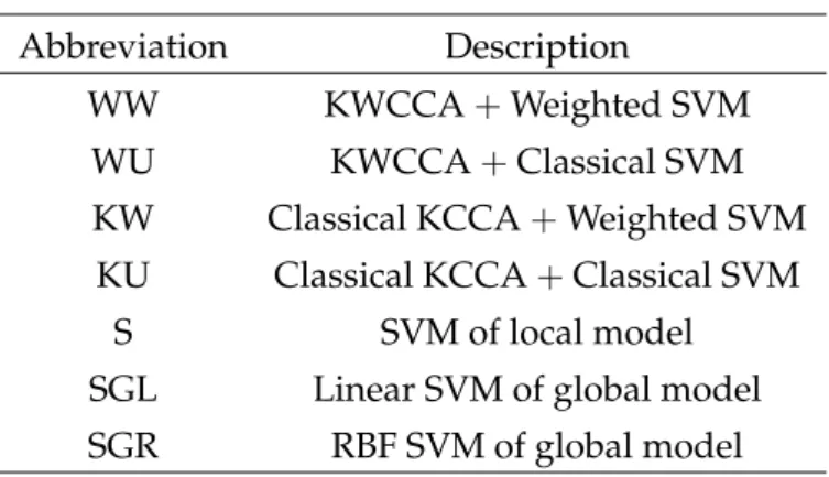
Table 3.1:Abbreviation of methods.
Abbreviation Description
WW KWCCA+Weighted SVM
WU KWCCA+Classical SVM
KW Classical KCCA+Weighted SVM KU Classical KCCA+Classical SVM
S SVM of local model
SGL Linear SVM of global model SGR RBF SVM of global model
of improvement in the performance of this algorithm if careful and suitable parameter selection is done.
For the global model, the kernel which achieves the best performance is the linear kernel. The regularization parameter is chosen asC=10, achieving the best performance among other values.
Results for the case of the RBF kernel with the best Cvalue obtained are also reported for comparison.
The methods based on KWCCA involve two stages upon implementation. First, we exploit KWCCA to extract a set of features for each compound. Second, we use them for training a machine learning algorithm employing SVMs before testing them to make predictions. In total, seven methods are implemented in the experiments: two using SVM in the global model setting, and the other five following the local model. One of the two global model methods uses RBF kernel for SVM, and the other uses the linear kernel. On the other hand, the methods used for the local models are as follows:
SVM, KCCA with classical SVM, KCCA with weighted SVM, KWCCA with classical SVM, and KWCCA with weighted SVM. For simplicity of notation, we shall refer to each of the seven methods using the abbreviations in Table3.1.
3.3.2 Performance Evaluation Criteria
The following criteria were used to compare the seven prediction methods:
1. Area under the ROC curve (AUC) – The receiver operating characteristic (ROC) curve is a plot of the true positive rate (TPR) versus the false positive rate (FPR) where
TPR= TP
TP+FN, FPR= FP FP+TN,
3.3 E X P E R I M E N T S A N D R E S U LT S 21
and TP, FN, FP, and TN are the number of true positives, false negatives, false positives, and true negatives, respectively.
For performance comparison using the ROC, the AUC value is further computed.
2. F-measure – A value which is given by the harmonic mean of precision and recall:
F= 2Prec×Recall Prec+Recall
where the precision Prec and the recall Recall are defined by Prec= TP
TP+FP and Recall= TP TP+FN,
respectively. Since the problem is presented as a binary classification problem, only the maximum value of the F- measure values for each target is considered. The scores obtained via SVM are used as confidence levels, thus, changing the threshold yields different predictions.
These values are calculated for each target protein and averaged over the ten data divisions. However, there are instances when the test set does not contain a true positive interaction, hence AUC and F-measures cannot be computed. Therefore, these values were disregarded and, out of 62 target proteins, AUC and F-measures were computed for 49 of them. The Wilcoxon signed test was used for the statistical significance of the difference among the values of the evaluation measures.
3.3.3 Effects of Using CCA and Weighting
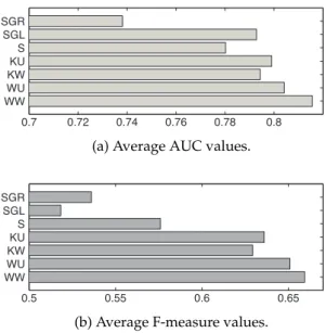
The average AUCs and F-measures are reported in Figures 3.3a and 3.3b, respectively. In comparison with the local models, four CCA-based methods, WW, WU, KW, and KU, achieve remarkably better AUCs and F-measures compared to those of S: the differences between the AUCs and F-measures of KW, the worst among the four CCA-based methods, and S are 0.014 and 0.053, respectively,
P-values:5.81×10⁻⁷and9.49×10−9respectively
. The AUC of the global model SGL is comparable to some of the local models, whereas the F-measure is not worse than that of S. A closer inspection on the results of SGL indicate that it has the lowest average number of true positives over all cross-validations among all models, around 161, which may be the reason behind a very small F-measure value.
22 P R E D I C T I N G P R O T E I N-L I G A N D I N T E R A C T I O N S
0.7 0.72 0.74 0.76 0.78 0.8 WW
WU KW KU S SGL SGR
(a) Average AUC values.
0.5 0.55 0.6 0.65
WW WU KW KU S SGL SGR
(b) Average F-measure values.
Figure 3.3:Average performance of the methods.Data was randomly split into training and test sets, and 10 training-testing data divisions were used for each method. Following the local model, AUC and F-measure were computed for each of the 62 targets. The bar plots represent the average AUC and average F-measure values, respectively, over the 10 cross validation sets and the 49 targets containing true positives. The two KWCCA-based methods, WW and WU, and the other methods were implemented for comparison. The difference of the performances of WW and WU from the other five methods showed to be statistically significant in terms of the P-values (by Wilcoxon signed rank test).
The effects of the weighted extension of CCA are manifested via comparison among four CCA-based methods. WW achieves significantly higher AUC and F-measures in average compared to KW and KU, where the P-values for the difference in the AUCs are 4.85×10⁻¹¹ and 6.91×10⁻¹⁰, and the P-values for the F-measures are3.59×10−7 and3.96×10−6, respectively.
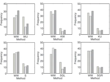
The frequencies of WW besting the AUC or F-measure values of the other methods in predicting interactions for a certain target protein are shown in the histograms in Figure3.4a. These values represent the number of target proteins such that the evaluated AUC and F-measure values for the method WW is better than the AUC and F-measure values of the other method in comparison. Instances when there are ties between the methods were unaccounted. For the evaluated AUC and F-measure values, WW outputs are more desirable than most of the others which indicates higher quality of prediction performance.
3.3 E X P E R I M E N T S A N D R E S U LT S 23
WW WU
0 10 20 30 40
Method
Frequency
WW KW
0 10 20 30 40 50
Method
Frequency
WW KU
0 10 20 30 40 50
Method
Frequency
WW S
0 10 20 30 40 50
Method
Frequency
WW SGL 0
10 20 30 40 50
Method
Frequency
WW SGR 0
10 20 30 40 50
Method
Frequency
(a) Histogram comparisons of the proposed method WW vs. other methods.
(b) Histogram comparisons of Weighted SVM using the weighting scheme in Equation (3.3) vs. Classical SVM.
Figure 3.4:Histograms illustrating the comparisons between the proposed method WW and other methods. Frequencies when the AUC, AUC between 0 and 0.05, and F-measure values of WW outperform the other methods, and vice-versa, are illustrated. It can be observed that AUC and F-measure values histograms for WW are more desirable than the rest.