Prof.FujioMINAMIProf.MasahitoUEDAProf.HidetoKANAMORIProf.MichioMATSUSHITA Thethesisjuryiscomposedof: Prof.MikioKOZUMA inpartialfullﬁllmentoftherequirementsforthedegreeofDoctorofPhilosophy,2007.Thisthesisissupervisedby: TheDepartmentofPhysicsTokyoInstitute

(1)

A thesis entitled

Electromagnetically Induced Transparency with Squeezed Vacuum

written by

Daisuke AKAMATSU

submitted to

The Department of Physics Tokyo Institute of Technology

in partial fullﬁllment of the requirements for the degree of Doctor of Philosophy,

2007.

This thesis is supervised by:

Prof. Mikio KOZUMA

The thesis jury is composed of:

Prof. Fujio MINAMI

Prof. Masahito UEDA

Prof. Hideto KANAMORI

Prof. Michio MATSUSHITA

(2)

(3)

Acknowledgement

It gives me great pleasure to express my deepest respect and sincere gratitude to Prof. Mikio Kozuma for his excellent guidance throughout the duration of this thesis work. His deep insight for getting to the heart of the problem and exceptional capacity to work has been a source of inspiration for me.

I am grateful to Prof. Akira Furusawa, Dr. Nobuyuki Takei, Mr. Hidehiro Yonezawa and Mr. Kentaro Wakui for their valuable comments and stim- ulating discussions on generation of a squeezed vacuum with sub-threshold optical parametric oscillator.

I am grateful to Prof. Takuya Hirano for his fruitful lecture on experimental quantum optics. The concept of a bichromatic homodyne method was born from his lecture.

I would like to thank Dr. Motonobu Kourogi and Dr. Kazuhiro Imai for helpful comments on feed-forward phase lock method.

I wish to express my appreciation to Prof. Hiroki Saito for discussing the mathematical issues on the experiments.

I would like to thank to Prof. Fujio Minami, Prof. Masahito Ueda, Prof.

Hideto Kanamori, and Prof. Michio Matsushita for their valuable comments on the thesis.

I also would like to thank one of my collaborators, Yoshihiko Yokoi, for making excellent electric circuits, which had an active part in our experimental setups.

I wish to express my gratitude to the members of Kozuma lab, Dr.

Koji Usami, Keiichirou Akiba, Norifumi Kanai, Takahito Tanimura, Jun- ichi Takahashi, Ryotaro Inoue, Kousuke Kashiwagi, and Toshiya Yonehara for sharing a great deal of fun time with me.

Special thanks goes to one of my best friends, Brett, who corrected many gramatical mistakes in this thesis and my girlfriend, Natsuki, whose presence is vital to the development of my creativity and humanity.

I must remember the blessings of my family members, who always sup- ported me. I am very much indebted to my parents for their endless sacriﬁce, love and aﬀection.

Finally, I would like to dedicate this thesis to my grandfather, who has always been in my center of heart.

Urawa, Saitama, Japan March, 2007

Daisuke Akamatsu

(4)

(5)

Introduction-scope of the thesis

The laser has been at the heart of various ﬁelds of research since its invention [1], because of its intensity and coherence. In fact, soon after the birth of the laser, its extraordinary intensity generated optical harmonics [2]. A nonlinear crystal pumped by an intense monochromatic (694.3 nm) laser emitted the second harmonic light (347.2 nm). Since Franken’s report, the refractive index and the absorption coeﬃcient of materials have had to be considered variable parameters. The paper marked the beginning of nonlinear optics.

This research was followed by a parametric ampliﬁcation [3], a parametric oscillation [4], a four wave mixing [5, 6], and so on. Recently optical comb generation [7], which plays the main role in frequency measurement of light [8]

has widely attracted attention. Optical comb generation is also an extension of the research.

Although P. A. M. Dirac found the beautiful quantum theory of radiation [9], all of the above phenomena can be explained by the semiclassical theory, in which light is treated as a classical electric ﬁeld. H. P. Yuen introduced the concept of a squeezed state, which one of the main topics in this thesis, and pointed out that the squeezed state can be generated through a degenerate parametric ampliﬁcation [10]. The squeezed state is one of the nonclassical states of light. As squeezed states have potential applications to optical communications [11] and gravitation radiation detectors [12], many experi- mentalists tried to generate the squeezed states. In 1986, R. E. Slusher, et.

al., succeeded in the generation of squeezed vacuum states through parametric ampliﬁcation using a Dye laser [13]. Squeezed vacuum states have less noise than a vacuum state in one of the ﬁeld quadratures. The squeezing level increased to 7dB with a sub-threshold parametric oscillator by 2006 [14].

The squeezed vacuum exhibits a number of quantum features and an EPR type-correlated beam can be produced by overlapping two squeezed vacua. Such an EPR beam plays the main role in quantum teleportation [15, 16, 17]. In 1998, A. Furusawa, et. al., successfully demonstrated the un- conditional quantum teleportation of a light [18]. Since S. L. Braunstein and his colleagues developed the quantum information theory with continuous variables [19, 20], the squeezed vacuum has been regarded as an important information carrier.

The other important property of the laser is coherence, which is used

for coherent manipulation and preparation of the medium. One of the early

applications is the photon echo, which was demonstrated in 1964 [21]. A

(8)

coherently prepared macroscopic electric dipole moment by first laser pulse restores the dephasing after the second laser pulse and emits an echo. The idea of the photon echo came from the spin echo [22], which had been inves- tigated in magneto-resonance. The success of the photon echo means that the laser can be used for the coherent manipulation of dipoles, in the same way as the coherent manipulation of spins by the magnetic field. The optical Bloch equation [23] shows a clear correspondence between atomic dipole manipulation by laser and spin manipulation by a magnetic field.

The optical reaction of atoms dramatically changes through laser-induced coherence of atomic states. The destructive quantum interference between the excitation amplitudes eliminates the absorption at the resonant frequency of a transition. This is referred to as electromagnetically induced transparency (EIT), which is another main issue in this thesis. EIT was ﬁrst observed by S. E. Harris and his colleagues in 1991 [24, 25]. EIT occurs in a three-level atomic system. When a weak probe light is incident on atoms which are irradiated by an intense control light, the transition amplitudes from the ground states to the excited state destructively interfere and the absorption of the probe light disappears as a result.

EIT provides many interesting phenomena, such as lasers without inver- sion [26, 27, 28], giant nonlinearity [29, 30, 31, 32], ultraslow light [33, 34, 35, 36], and so on. EIT can also be explained by the semiclassical theory and all of these experiments have been carried out with laser lights, or lights in a coherent state.

M. Fleishhauer and M. D. Lukin treated the probe light as a quantized ﬁeld and gave the quantum description of the probe light in an EIT medium.

The description is termed a dark state polariton [37, 38]. They also found that the speed of the dark state polariton can be controlled by the intensity of the control light and can be stopped by turning oﬀ the control light. The stopped dark state polarition can be accelerated by turning on the control light again, and the probe light is retrieved from the medium. The whole process is unitary, therefore ideally the quantum information of photons can be stored in the EIT medium. This is called storage of light technique. This paper has attracted attention to the EIT, because the paper provides an easier way to quantum memory.

Quantum Memory — motivation and world trend —

While photons are the fastest and very robust carriers of quantum information, they do not interact with each other and are diﬃcult to localize. In contrast, atoms can interact with each other and can even be stopped by conventional laser cooling techniques but they are not fast carriers of information (Fig1). Therfore one would like to employ atoms to manipulate and store quantum information and photons to carry the information from atoms to atoms. Such a system is termed a quantum network, which was ﬁrst proposed by J. I. Cirac [39].

A single photon state is often used as a qubit state and is one of the most important ingredients in quantum communications. A conceptually

8

(9)

Fastest Carrier Can not be localized Robust

Easy to measure quantum state

Can be localized Interactive Hard to measure quantum state

2JQVQP #VQO

3W CP VW O /G OQ T[

Figure 1: Schematic image of light-atom interface. The disadvantage of photons can be conpensated with atoms, and vice versa. As quantum memory connencts these two feilds, we can cancel the disadvantages of both systems and utilize only advantages with quantum memory.

simple approach to the quantum memory of a single photon is to employ a single two-level atom. It is possible to store and retrieve a single photon state through coherent absorption and emission of a single photon. The interaction Hamiltonian of this process is given by

H = gˆ aˆ σ 12 + h.c., (1)

where ˆ a is the annihilation operator of the light and ˆ σ ₁₂ is the ﬂipping operator from the atomic states | 2 ⟩ to | 1 ⟩ . The interaction strength g is very weak, so placing the atom in a high-Q optical resonator is necessary to ef- fectively increase the interaction [40, 41, 42]. Despite the enormous experimental progress in this ﬁeld it is technically very challenging to achieve the necessary strong-coupling regime [43, 44, 46].

The proposal by M. Fleischhauer and M. D. Lukin [37, 38] is based on an adiabatic transfer of the quantum state of photons to collective atomic excitations with EIT. A collective atomic operator [47] is deﬁned by the sum of the ﬂipping operators of every atom as follows:

˜

σ ₁₂ = 1

√ N

∑

j

ˆ

σ ₁₂ ^(j) . (2)

Here N represents the number of atoms. The Hamiltonian describing the interaction between light and atoms is given by

H = g √

N a ˆ σ ˜ ₁₂ + h.c.. (3)

The interaction strength between the light and the collective atomic excitation is √

N times as large as that between the light and a single atom. This

alleviates the experimental requirements with a single-atom cavity QED. In

fact, preliminary demonstrations of the proposal were soon carried out inde-

pendently by two groups [48, 49]. One of the groups also demonstrated that

the phase of the stored pulse can be manipulated by applying a magnetic

ﬁeld during storage [50].

(10)

#WUVTCNKC 2-.CO#07 4D

̌UVQTCIGQHUSGWW\GFXCEWWO̍

75#

.8*CW*CTXCTF 0C$'%

̌.KIJVCPF/CVVGTYCXGKPVGTHCEG̍

,CRCP

/-Q\WOC6+6GEJ 4D

̌UVQTCIGQHUSWGG\GFXCEWWO̍

&GPOCTM

'52QN\KM#CTJWU

%U

̌3WCPVWOOGOQT[YKVJ30&̍

75#

/&.WMKP*CTXCTF 4D

̌UVQTCIGQHUKPINGRJQVQPU̍

75#

#-W\OKEJ)+6 4D/16

̌UVQTCIGQHUKPINGRJQVQPU̍

'+6ITQWRU

1RVKECNJQOQF[PG

2JQVQEQWPVKPI

Figure 2: Some groups on quantum memory with atomic ensembles.

Recently several groups have succeeded in storing and retrieving light of single photons with storage of light technique [51, 52]. These experiments have demonstrated nonclassical characteristics of the retrieved light ﬁeld, such as photon antibunching and violation of classical inequalities. Although their demonstrations are large steps towards scalable quantum information processing with single photons, it should be noted that the advantage of quantum memory with atomic ensembles is not only its simplicity of im- plimantation but also its storage capacity. While one can store only single photons with single atoms in a high-Q cavity, atomic ensembles can be used for storage of arbitrary states of photons ¹ .

Arbitrary states of photons can be converted into those of atoms and vice versa with “genuine” quantum memory, that is, the “genuine” quantum memory connects these two fields. In order to verify such a quantum memory, one has to estimate the density matrix of the light by using homodyne detection. Note that, unlike a photon counting method, homodyne detection is sensitive to the vacuum state. E. S. Polzik and his colleagues are trying to map an arbitrary quantum state of light onto an atomic ensemble from another approach. They utilize quantum nondemolition measurement of atomic spins [53, 54] and verified storage of a coherent state of light with a homodyne method [55], however, their method does not restore the stored state as a radiation field. While some improvement of the system is needed to retrieve the stored state as radiation field [56], the EIT approach can be used for “genuine” quantum memory as it is. Figure 2 schematically shows some groups working on quantum memory with atomic ensembles on the world map.

For demonstration of “genuine” quantum memory with EIT, we adopted a squeezed vacuum state as an input state. The squeezed vacuum carries

1

Stricktly speaking, the number of stored photons must be much less than that of atoms.

10

(11)

lower quadrature noise than the coherent state, therefore after storage of the squeezed vacuum, the spin noise of the atomic system is reduced. Such a state is termed “spin squeezed state” [57] and has attracted much attentions [58, 59, 60]. Recently the squeezed vacuum was employed for generation of Schr¨ odinger kitten state [61, 62], therefore storage of squeezed vacuum will leads us to Schr¨ odinger kitten state of atomic systems. The storage of the squeezed vacuum will open the door to a new stage of quantum manipulation of lights and atoms.

The experiment in this thesis is a milestone in the storage of a squeezed vacuum. The thesis is divided into two parts:

• Generation of a Squeezed Vacuum with Periodically Poled KTiOPO ₄ crystals

• Electromagnetically Induced Transparency with a Squeezed Vacuum

In Chapter 1, the basic concept of a squeezed vacuum is presented. To observe a quadrature noise, a balanced homodyne method has been employed for a long time. The theory of the homodyne method is also presented.

In Chapter 2, the experiment on generation of squeezed vacuum resonant on rubidium D ₁ line is reported. At the beginning of the research, there were no reports on generation of squeezed vacuum resonant on rubidium. We have developed two methods; one is with periodically poled lithium niobate waveguides, which is not written in this thesis, the other method is with periodically poled KTiOPO ₄ crystals in cavities. The observed squeezing level − 2.75 dB was the world record at that time. This experimental results can be also seen in [63]

In Chapter 3, the experiment on electromagnetically induced transparency with a squeezed vacuum is presented. This experiment was the ﬁrst demonstration of EIT with a quantum probe light. A theory of EIT with a quantum probe light is presented before the details of the experiment. The experimental results can also be seen in [64]

In Chapter 4, the experiment on observation of ultraslow propagation of a

squeezed vacuum is presented. To observe the squeezed vacuum after passing

through the sub-MHz EIT window, we developed a new homodyne method,

which enables us to observe the quadrature squeezing of the carrier frequency

component. With the new homodyne method, we observed the delay of the

squeezed vacuum by 1.3 µs. Although there are a few reports on the delay of

nonclassical light[65, 66], the obtained delay time in our experiment is quite

larager than the previous ones.

(12)

(13)

Part I

Generation of Squeezed vacuum

(14)

(15)

Chapter 1 Squeezed State

In this chapter, the concept of a squeezed vacuum state is presented. A single- mode squeezed state reduces the ﬁeld quadrature noise for a certain direction in the phase-space. The single-mode theory is expanded to the two-mode theory, in which the concept of two-mode quadrature is introduced. A two- mode squeezed state is deﬁned as the state, of which two-mode quadrature noise is lower than the vacuum state.

In order to observe a squeezed vacuum, a balanced homodyne method has been employed for a long time. It should be noted that not a single- single mode quadratrure noise but a two-mode quadrature noise is measured with the conventional homodyne method. A theoritical treatment for the homodyne method is also presented in this chapter.

1.1 Single-mode Electric Field Theory

A quantized single-mode electric ﬁeld (in a Heisenberg picture) is written as E(z, t) = ˆ 1

2 [√ 2 ~ ω

ε ₀ V ˆ a exp( − i(ωt − kz)) + h.c.

]

, (1.1)

where ω, k and V are the angular frequency, the wave number of the field, and the quantization mode volume, respectively. ˆ a is an annihilation operator of the field and satisfies the following commutation relation,

[ˆ a, ˆ a

^†

] = 1. (1.2)

(1.1) can be transformed into E(z, t) = ˆ

√ 2 ~ ω ε ₀ V

[ x ˆ

ϕ

cos(ωt − kz − ϕ) + ˆ x

_ϕ+π/2

sin(ωt − kz − ϕ) ]

, (1.3) with quadrature operators deﬁned as

ˆ

x

ϕ

= ˆ ae

⁻^iϕ

+ ˆ a

^†

e

^iϕ

2 , (1.4)

ˆ

x

_ϕ+π/2

= ˆ ae

⁻^iϕ

− ˆ a

^†

e

^iϕ

2i . (1.5)

(16)

The commutation relation between the quadratures is given by [ˆ x

_ϕ

, x ˆ

_ϕ+π/2

] = i

2 . (1.6)

Therefore the uncertainty relation is written as

⟨ (∆x

_ϕ

) ² ⟩ ⟨

(∆x

_ϕ+π/2

) ² ⟩

≥ 1

16 , (1.7)

where the noise or the variance of the quadrature is deﬁned as

⟨ (∆ˆ x

ϕ

) ² ⟩

= ⟨ ˆ x ²

_ϕ

⟩

− ⟨ x ˆ

ϕ

⟩ ² . (1.8)

1.1.1 Single-mode Vacuum State

The vacuum state | 0 ⟩ is deﬁned as ˆ

a | 0 ⟩ = 0. (1.9)

The expectation value of the electric ﬁeld and the square of the electric ﬁeld are calculated as

⟨ 0 | E ˆ | 0 ⟩ = 0, (1.10)

⟨ 0 | E ˆ ² | 0 ⟩ = ~ ω

2ϵ ₀ V , (1.11)

respectively. Therefore the noise of the electric ﬁeld is given by

⟨ 0 | (∆ ˆ E) ² | 0 ⟩ = ~ ω

2ϵ 0 V . (1.12)

The expectation value of the quadrature, the square of the quadrature, and the quadrature noise are given by

⟨ 0 | x ˆ

_ϕ

| 0 ⟩ = 0, (1.13)

⟨ 0 | x ˆ ²

_ϕ

| 0 ⟩ = 1

4 , (1.14)

⟨ 0 | (∆ˆ x

_ϕ

) ² | 0 ⟩ = 1

4 , (1.15)

respectively. Since the vacuum state satisﬁes the equality of (1.7), the vacuum state is one of the minimum uncertainty state with respect to the quadrature.

1.1.2 Single-mode Coherent State

One of the quantum states, which seems closest to a classical picture, is called a coherent state. A coherent state is deﬁned by a displacement operator

D(α) = exp ˆ (

αˆ a

^†

− α

^∗

ˆ a )

, (1.16)

16

(17)

where α = | α | e

^iθ

. The displacement operator displaces the annihilation operator (creation operator) by α (α

^∗

) ¹

D ˆ

^†

(α)ˆ a D(α) = ˆ ˆ a + α, (1.17) D ˆ

^†

(α)ˆ a

^†

D(α) = ˆ ˆ a

^†

+ α

^∗

. (1.18) The coherent state | α ⟩ is given by operating the displacement operator to the vacuum state,

| α ⟩ = ˆ D(α) | 0 ⟩ . (1.19) Since the quadrature noise of the light in a coherent state is given by

⟨ α | (∆ˆ x

_ϕ

) ² | α ⟩ = 1

4 , (1.20)

the coherent state is also one of the minimum uncertainty state. The expectation value of the electric ﬁeld of a coherent state is given by

⟨ α | E ˆ | α ⟩ =

√ 2 ~ ω

ϵ ₀ V | α | cos(ωt − kz − θ). (1.21) The electric ﬁeld is proportional to | α | . The square of the electric ﬁeld for the coherent state is given by

⟨ α | E ˆ ² | α ⟩ = ~ ω 2ϵ ₀ V

[ 4 | α | ² cos ² (ωt − kz − θ) + 1 ]

, (1.22)

and the noise of the electric ﬁeld is written as

⟨ α | (∆ ˆ E) ² | α ⟩ = ~ ω

2ϵ ₀ V . (1.23)

It should be noted that the noise of the electric field of the coherent state is independent on | α | and the same as that of the vacuum state. Since the amplitude of the electric field is proportional to | α | , the ratio of the electric field noise to the amplitude of the field is 1/ | α | . This means that the noise of the electric field, which originates the quantization, can be ignored when the light in a coherent state is intense enough. A laser is known as one of the lights in a coherent state.

1.1.3 Single-mode Squeezed State

The quantum theory does not restrict the way to distribute the quadrature noise. We can consider such a state that ⟨ (∆ˆ x

_ϕ

) ² ⟩ is smaller than 1/4 while

⟨ (ˆ x

_ϕ+π/2

) ² ⟩

is larger than 1/4. Such states is called a squeezed state. A single-mode squeezed state is deﬁned by

| ψ ⟩

S

= ˆ S

S

(η) | 0 ⟩ , (1.24)

1

We can prove the formula with Baker-Hausdorﬀ formula: exp(ξ A) ˆ ˆ B exp( − ξ A) = ˆ ˆ B +

ξ[ ˆ A, B] + ˆ

^ξ_2!²

[ ˆ A, [ ˆ A, B]] + ˆ

^ξ_3!³

[ ˆ A, [ ˆ A, [ ˆ A, B]]] + ˆ · · · +

^ξ_n!ⁿ

[ ˆ A, [ ˆ A, [ ˆ A, . . . [ ˆ A, B]]]] + ˆ · · · .

(18)

(a) (b) (c)

Figure 1.1: Phase-space image showing the uncertainty in (a) a single-mode vacuum state | 0 ⟩ , (b) a single-mode coherent state | α ⟩ , and (c) a single-mode squeezed state | ψ ⟩ .

with a unitary squeezing operator S ˆ

S

(η) ≡ exp

[ 1 2

[ η

^∗

a ˆ ² − η(ˆ a

^†

) ² ]]

, η = re

^iθ

, (1.25)

where r is called a squeezing parameter. The squeezing operator has the following useful transformation properties

S ˆ

S^†

(η)ˆ a S ˆ

S

(η) = ˆ a cosh r − ˆ a

^†

e

^iθ

sinh r, (1.26) S ˆ

_S^†

(η)ˆ a

^†

S ˆ

S

(η) = ˆ a

^†

cosh r − ˆ ae

⁻^iθ

sinh r. (1.27) The expectation values of the quadrature x

_ϕ

for the squeezed state is given by

S

⟨ ψ | x ˆ

_ϕ

| ψ ⟩

S

= 0, (1.28)

S

⟨ ψ | x ˆ ²

_ϕ

| ψ ⟩

S

= 1

4 (cosh 2r − cos(θ − 2ϕ) sinh 2r). (1.29) When θ = 2ϕ, the quadrature noise are simply written as

S

⟨ ψ | (∆ˆ x

_ϕ

) ² | ψ ⟩

_S

= 1

4 e

⁻

^2r , (1.30)

S

⟨ ψ | (∆ˆ x

_ϕ+π/2

) ² | ψ ⟩

S

= 1

4 e ^2r . (1.31)

This state satisﬁes (1.7), i.e., the squeezed state is also one of the minimum uncertainty states and the quadrature noise ⟨ (∆ˆ x

_ϕ

) ² ⟩ is less than that of the vacuum state when r > 0.

18

(19)

1.2 Two-mode Electric Field theory

The two-mode ﬁeld consisting of ω ± δ can be written as E(z, t) = ˆ 1

2 √ 2

√ 2 ~ ω

ε ₀ V [ˆ a

_ω+δ

exp( − i((ω + δ)t − kz)) + h.c.]

+ 1

2 √ 2

√ 2 ~ ω

ε 0 V [ˆ a

_ω₋_δ

exp( − i((ω − δ)t − kz)) + h.c.] . (1.32) The commutation relations between the ﬁeld operators are given by

[ ˆ

a

_ω_±_δ

, a ˆ

^†_ω_±_δ

]

= 1, (1.33)

[ ˆ

a

_ω_±_δ

, a ˆ ⁽

_ω^†_∓

⁾

_δ

]

= 0. (1.34)

(1.32) can be rewritten as E(z, t) = ˆ

√ 2 ~ ω ε ₀ V

[ X(δ, ϕ) cos(ωt ˆ − kz − ϕ) + ˆ X(δ, ϕ + π/2) sin(ωt − kz − ϕ) ]

. (1.35) Here the (Hermite) two-mode quadrature phase amplitudes are

X(δ, ϕ) = ˆ a ˆ

_ω+δ

e

⁻^i(δt+ϕ)

+ ˆ a

^†_ω+δ

e

^i(δt+ϕ)

+ ˆ a

_ω₋_δ

e

⁻ⁱ⁽⁻^δt+ϕ)

+ ˆ a

^†_ω₋_δ

e

ⁱ⁽⁻^δt+ϕ)

2 √

2 ,

(1.36) X(δ, ϕ ˆ + π/2) = a ˆ

_ω+δ

e

^−i(δt+ϕ)

− ˆ a

^†_ω+δ

e

^i(δt+ϕ)

+ ˆ a

_ω₋_δ

e

^{−i(−δt+ϕ)}

− ˆ a

^†_ω₋_δ

e

^i(−δt+ϕ)

2 √

2i .

(1.37) The commutation relation between two-mode quadratures is given by

[ ˆ X(δ, ϕ), X(δ, ϕ ˆ + π/2)] = i

2 , (1.38)

and the uncertainty inequality is written as

⟨

(∆ ˆ X(δ, ϕ)) ²

⟩ ⟨

(∆ ˆ X(δ, ϕ + π/2)) ²

⟩ ≥ 1

16 . (1.39)

1.2.1 Two-mode Squeezed State

In the previous section, we discussed a squeezed vacuum state consisting of a single mode ˆ a. In this section, we expand the concept to the two-mode state. The two-mode squeezed vacuum is deﬁned as

| ψ ⟩

T

= ˆ S

T

(η) | 0 ⟩ , (1.40) where a two-mode squeezing operator ˆ S

T

is given by

S ˆ

T

(η) ≡ exp(η

^∗

ˆ a

ω+δ

a ˆ

ω−δ

− ηˆ a

^†_ω+δ

ˆ a

^†_ω₋_δ

), η = re

^iθ

. (1.41)

(20)

The following commutation relation

[ηˆ a

^†_ω+δ

ˆ a

^†_ω₋_δ

− η

^∗

ˆ a

_ω+δ

ˆ a

_ω₋_δ

, ˆ a

_ω_±_δ

] = − ηˆ a

^†_ω_∓_δ

, (1.42) generates a useful formula

S ˆ

_T^†

(η)ˆ a

_ω_±_δ

S ˆ

T

(η) = exp(ηˆ a

^†_ω+δ

ˆ a

^†_ω₋_δ

− η

^∗

ˆ a

_ω+δ

ˆ a

_ω₋_δ

)ˆ a

_ω_±_δ

exp(η

^∗

ˆ a

_ω+δ

a ˆ

_ω₋_δ

− ηˆ a

^†_ω+δ

ˆ a

^†_ω₋_δ

)

= ˆ a

_ω_±_δ

+ [ηˆ a

^†_ω+δ

ˆ a

^†_ω₋_δ

− η

^∗

ˆ a

_ω+δ

ˆ a

_ω₋_δ

, ˆ a

_ω_±_δ

] + 1

2! [ηˆ a

^†_ω+δ

ˆ a

^†_ω₋_δ

− η

^∗

ˆ a

_ω+δ

a ˆ

_ω₋_δ

, [ηˆ a

^†_ω+δ

ˆ a

^†_ω₋_δ

− η

^∗

a ˆ

_ω+δ

ˆ a

_ω₋_δ

, ˆ a

_ω_±_δ

]] + · · ·

= ˆ a

_ω_±_δ

− ηˆ a

^†_ω_∓_δ

+ 1

2! ηη

^∗

ˆ a

_ω_±_δ

− 1

3! η ² η

^∗

a ˆ

^†_ω_∓_δ

+ 1

4! η ² η

^∗

² ˆ a

_ω_±_δ

− · · ·

= ˆ a

_ω_±_δ

− re

^iθ

ˆ a

^†_ω_∓_δ

+ 1

2! r ² a ˆ

_ω_±_δ

− 1

3! r ³ e

^iθ

ˆ a

^†_ω_∓_δ

+ 1

4! r ⁴ a ˆ

_ω_±_δ

− · · ·

= ˆ a

_ω_±_δ

cosh r − ˆ a

^†_ω_∓_δ

e

^iθ

sinh r, (1.43) with Baker-Hausdorﬀ formula.

Since the expectation values of the two-mode quadrature noise and the square thereof are written as

T

⟨ ψ | X(δ, ϕ) ˆ | ψ ⟩

T

= 0, (1.44)

T

⟨ ψ | X ˆ ² (δ, ϕ) | ψ ⟩

T

= 1

4 (cosh 2r − cos(θ − 2ϕ) sinh 2r), (1.45) respectively, the two-mode quadrature noise is given by

T

⟨ ψ | (∆ ˆ X(δ, ϕ)) ² | ψ ⟩

T

= 1

4 (cosh 2r − cos(θ − 2ϕ) sinh 2r) . (1.46) When θ = 2ϕ, the quadrature noise is written as

T

⟨ ψ | (∆ ˆ X(δ, ϕ)) ² | ψ ⟩

T

= 1

4 e

^−2r

, (1.47)

T

⟨ ψ | (∆ ˆ X(δ, ϕ + π/2)) ² | ψ ⟩

T

= 1

4 e ^2r . (1.48)

The quadrature noise of the two-mode vacuum state is given by

T

⟨ 0 | (∆ ˆ X(δ, ϕ)) ² | 0 ⟩

T

= 1

4 , (1.49)

therefore

⟨

(∆ ˆ X(δ, ϕ)) ²

⟩

is smaller than that of vacuum state, when r > 0.

1.3 Balanced Homodyne Method with Monochro- matic Local Oscillator

In order to measure the quadarature noise of a signal light, an optical balanced homodyne method has been employed for a long time. The method is schematically shown in Fig. 1.3. A signal beam ˆ a _S is mixed on the beam

20

(21)

(a) (b)

Figure 1.2: Phase-space image showing the uncertainty in (a) a two-mode vacuum state | 0 ⟩ , (b) a two-mode squeezed state | ψ ⟩ .

Spectrum Analyzer

PD A

PD B BS

Figure 1.3: A schematic of a homodyne method. A local oscillator light

is in a single-mode coherent state. The power of the diﬀerential current is

measured by a spectrum analyzer.

(22)

Local Oscillator

Squeezed Vacuum

Frequency

Measured Components

Figure 1.4: Schematic image of a homodyne method with a monochromatic local oscillator. The measured frequency components of the squeezed vacuum are ω ± δ.

splitter with a monochromatic local oscillator ˆ a _LO in a coherent state. Each output ˆ a _A,B is detected by the photodetectors A and B, respectively, and the power spectrum of the diﬀerential current is measured by a spectrum analyzer. From the input-output relation of the beam splitter, the output ﬁelds can be written as

ˆ

a A (t) = 1

√ 2 { ˆ a LO (t) + iˆ a S (t) } , (1.50) ˆ

a _B (t) = 1

√ 2 { iˆ a _LO (t) + ˆ a _S (t) } , (1.51) respectively. Since the local oscillator light is in a coherent state, the annihilation operator of the ﬁeld can be treated as a complex variable

ˆ

a LO (t) = αe

⁻^iωt

, (1.52)

α = | α _mono | e

^iθ

. (1.53)

Usually a squeezed vacuum generated by nonlinear crystal is broad (∆ω >

10MHz). We can, however, ignore the frequency components of the signal ﬁeld other than ˆ a

_ω_±_δ

e

^i(ω^±^δ)t

, since the spectrum analyzer measures a power of a beat δ (Fig. 1.4). Therefore the signal ﬁeld can be written as

ˆ

a _S (t) = ˆ a

_ω+δ

e

⁻^i(ω+δ)t

+ ˆ a

_ω₋_δ

e

⁻^i(ω⁻^δ)t

. (1.54) (1.52) and (1.54) are substituted into (1.50) and (1.51), and we obtain

ˆ

a _A (t) = 1

√ 2 (αe

⁻^iωt

+ iˆ a

_ω+δ

e

⁻^i(ω+δ)t

+ iˆ a

_ω₋_δ

e

⁻^i(ω⁻^δ)t

), (1.55) ˆ

a _B (t) = 1

√ 2 (iαe

⁻^iωt

+ ˆ a

_ω+δ

e

⁻^i(ω+δ)t

+ ˆ a

_ω₋_δ

e

⁻^i(ω⁻^δ)t

). (1.56)

22

(23)

The diﬀerential current between PD A and PD B is given by

∆ ˆ I = C(ˆ a

^†

_A (t)ˆ a _A (t) − ˆ a

^†

_B (t)ˆ a _B (t))

= iC[(α

^∗

ˆ a

_ω+δ

− αˆ a

^†_ω₋_δ

)e

⁻^iδt

+ (α

^∗

ˆ a

_ω₋_δ

− αˆ a

^†_ω+δ

)e

^iδt

]

= C | α _mono | [ˆ a

_ω+δ

e

⁻^i(δt+(θ⁻^π/2))

+ ˆ a

^†_ω+δ

e

^i(δt+(θ⁻^π/2))

+ ˆ a

_ω₋_δ

e

⁻ⁱ⁽⁻^δt+(θ⁻^π/2))

+ ˆ a

^†_ω₋_δ

e

ⁱ⁽⁻^δt+(θ⁻^π/2))

]

= 2 √

2C | α _mono | X(δ, θ ˆ − π/2), (1.57) where two-mode quadrature ˆ X(δ, θ) is deﬁned by (1.37). According to the Wiener-Khintchine theorem, the spectral density function

⟨ S ˆ _mono

⟩

of ∆ ˆ I is given by

⟨ S ˆ _mono (δ

^′

)

⟩

= 1 π

∫

_∞

−∞

dτ

⟨

∆ ˆ I (t)∆ ˆ I(t + τ )

⟩

cos δ

^′

τ. (1.58) Substituting (1.57) into (1.58), we obtain

⟨ S ˆ _mono (δ

^′

)

⟩

= 8(C | α _mono | ) ²

⟨ X ˆ ² (δ, θ − π/2)

⟩

δ(δ

^′

− δ), (1.59) where δ(δ

^′

− δ) is the Dirac delta function. If the signal ﬁeld is in a vacuum state, the measured noise is given by

⟨ S ˆ _mono (δ, θ) ⟩ vac = 2(C | α _mono | ) ² . (1.60) The power spectrum of the diﬀerential current normalized by vacuum noise level is given by

S ˆ mono (δ, θ) = 4 ˆ X ² (δ, θ − π/2). (1.61) It should be noted that the quadrature noise of various directions can be measured by changing the phases of the local oscillator.

When the signal state | ψ ⟩ is a two-mode squeezed vacuum state, the expectation value of the power spectrum is written as

⟨ ψ | S ˆ mono (δ, θ) | ψ ⟩ = cosh 2r − cos(ϕ − 2θ + π) sinh 2r. (1.62) As discussed in the next chapter, ϕ represents the phase of the pump ﬁeld in the optical parametric ampliﬁer. Without any loss of generality, we can set ϕ = π. Figure 1.5 shows the dependence of the normalized noise power on the phase of the local oscillator θ when the squeezing parameter r = 0.3. The maximum squeezing ( − 2.6 dB) and antisqueezing (+2.6 dB) can be observed when θ = 0 and θ = π/2, respectively.

Spatial overlapping of signal beam with local oscillator

In the previous discussion, we did not consider the spatial modes of the

signal light and the local oscillator light, which has, implicitly, been assumed

to be exactly the same. As the homodyne method measures the quadrature

(24)

0 1 2 3

-3 -2 -1

antisqueeze

squeeze

Th e N o rma lized Noise Power (dB)

Figure 1.5: The dependence of the normalized power on the phase of the local oscillator with the picture of the phase space image. The squeezing parameter r=0.3. The normalized noise power is usually expressed with the unit of dB, i.e., 10 log ₁₀

⟨ S ˆ

⟩ (dB).

24

(25)

noise of the ﬁeld of the same spatial mode as that of the local oscillator, the spatial overlapping between the signal light and the local oscillator is very important. Let ξ be the spatial overlap of the local oscillator with the signal beam ² . The local oscillator is devided into the two modes.

ˆ

a _LO = ξˆ a

^∥

_LO + √

1 − ξ ² ˆ a

^⊥

_LO , (1.63) where the spatial mode of ˆ a

^∥

_LO is exactly same as the signal beam, whereas the spatial mode of ˆ a

^⊥

_LO is orthogonal to that of the signal beam. (1.50) and (1.51) can also devided into two modes

ˆ

a

^∥

_A (t) = 1

√ 2 { ˆ a

^∥

_LO (t) + iˆ a

^∥

_S (t) } , (1.64) ˆ

a

^∥

_B (t) = 1

√ 2 { iˆ a

^∥

_LO (t) + ˆ a

^∥

_S (t) } , (1.65) ˆ

a

^⊥

_A (t) = 1

√ 2 { ˆ a

^⊥

_LO (t) + iˆ a

^⊥

_S (t) } , (1.66) ˆ

a

^⊥

_B (t) = 1

√ 2 { iˆ a

^⊥

_LO (t) + ˆ a

^⊥

_S (t) } . (1.67) The parallel and orthogonal annihilation operators of the local oscillator in a coherent state are written as

ˆ

a

^∥

_LO (t) = ξαe

^−iωt

, (1.68)

ˆ

a

^⊥

_LO (t) = √

1 − ξ ² αe

⁻^iωt

, (1.69) respectively. The power of the diﬀerential current can be given by

S ˆ _mono (δ, θ) = ξ ² S ˆ _mono

^∥

(δ, θ) + (1 − ξ ² ) ˆ S _mono

^⊥

(δ, θ), (1.70) with

S ˆ _mono

^∥

⁽

^⊥

⁾ (δ, θ) = 8(C | α _mono | X ˆ

^∥

⁽

^⊥

⁾ (δ, θ)) ² , (1.71) where ˆ X

^∥

⁽

^⊥

⁾ represents the quadrature noise of the mode parallel (orthogonal) to the local oscillator. Since the state, to which ˆ X

^⊥

operates, is a vacuum, the normalized power spectrum of the diﬀerential current is given by

S ˆ mono (δ, θ) = 4ξ ² ( ˆ X

^∥

(δ, θ)) ² + 1 − ξ ² . (1.72) The above discussion can be expanded to the case which a squeezed vacuum experiences the intensity loss L before the homodyne detector. The expression of the normalized power spectrum is written as

S ˆ mono (δ, θ) = 4ζ( ˆ X

^∥

(δ, θ)) ² + 1 − ζ, (1.73)

where we introduce the detection eﬃciency factor ζ = (1 − L)ξ ² . Figure

1.6 shows the dependence of the power spectrum on the phase of the local

oscillator θ when the squeezing parameter r = 0.3, the visibililty ξ = 0.95,

(26)

0 1 2 3

-3 -2 -1

antisqueeze

squeeze

Th e N o rma lized Noise Power (dB)

Figure 1.6: The dependence of the power spectrum on the phase of the local oscillator with the picture of the phase space image. The squeezing parameter r = 0.3, the visibililty ξ = 0.95, and the loss L = 0.2.

and the loss L = 0.2. The maximum squeezing ( − 1.7 dB) and antisqueezing (+2.0 dB) is observed by varying the phase of the local oscillator. It should be noted that the squeezing level decreases by 0.9 dB (=2.6dB − 1.7dB), while the antisqueezing level decreases by only 0.6 dB (=2.6 dB − 2.0 dB).

The squeezing is more sensitive to the optical loss or visibility than the anitsqueezing.

This fact can be understood as follows. In quantum theory of radiation, the loss means not only reduction of the number of the photons, but also invasion of the vacuum noise. Consider a pure squeezed vacuum of which quadrature noises are given

⟨ x ˆ ²

_ϕ

⟩

= 1 8

(

= 1

2 × ⟨ 0 | x ˆ ²

_ϕ

| 0 ⟩ )

, (1.74)

⟨ x ˆ ²

_ϕ+π/2

⟩

= 1 2

( = 2 × ⟨ 0 | x ˆ ²

_ϕ

| 0 ⟩ )

, (1.75)

respectively. In other words, the squeezing and the antisqueezing level of the squeezed vacuum are − 3.0 dB and +3.0 dB, respectively. If half of the squeezed vacuum is absorbed and the vacuum noise is injected to the state

2

ξ is also called as a visibility.

26

(27)

(+3.0 dB)

(-3.0 dB)

(0 dB)

(0 dB) (-1.2 dB)

(+1.8 dB)

Figure 1.7: Schematic diaglam of loss. The − 3dB-squeezed vacuum passes through the loss L = 0.5. After the absorption, the observed squeezing level is decreases to − 1.2 dB.

(Fig. 1.7), the quadrature noise changes to

⟨ x ˆ ²

_ϕ

⟩

→ 0.5 × 1

8 + 0.5 × 1 4 = 3

16 , (1.76)

⟨ x ˆ ²

_ϕ+π/2

⟩

→ 0.5 × 1

2 + 0.5 × 1 4 = 3

8 , (1.77)

respectively. In other words, the squeezing and the antisqueezing level of the squeezed vacuum changes − 1.2 dB and + 1.8 dB, respectively. While the squeezing level changes by 1.8 dB, the antisqueezing level decreases by only 1.2 dB. This diﬀerence increases if the initial squeezing level is higher. A high level squeezed vacuum is very sensitive to optical loss. From a simple consideration, more than − 3 dB squeezing can not be obtained with the existence of 50%-loss.

The dependences of the maximum squeezing and antisqueezing on the detection eﬃciency are shown in Fig. 1.8 with the squeezing parameter r = 0.3.

antisqueezing

squeezing

0 0.2

0.4 0.6 0.8 1

1 2 3

-3 -2 -1

No rm ali zed No ise Power (dB)

Figure 1.8: The dependence of the power spectrum on the detection eﬃciency

ζ. The squeezing parameter r = 0.3.

(28)

(29)

Chapter 2 Generation of a Squeezed Vacuum Resonant on

Rubidium with Periodically Poled KTiOPO ₄

We succeeded in the generation of a continuous-wave squeezed vacuum resonant on the Rb D ₁ line (795nm) using periodically poled KTiOPO ₄ crystals in cavities. We observed a squeezing level of − 2.75 ± 0.14 dB and an antisqueezing level of +7.00 ± 0.13 dB.

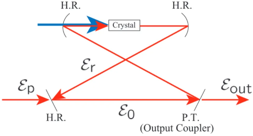
To generate a squeezed vacuum, we have to construct two inevitable parts, i.e., a doubler, and an optical parametric ampliﬁer (squeezer). The theory of the second nonlinear optics in the cavity is presented before the details of the experiment.

2.1 Formalism of Wave Propagation in Non- linear Medium[68]

First we derive equations describing a light propagating in a nonlinear medium.

Generally the polarization of a medium loses proportionality to the ﬁeld un- der an intense light. Such an intense light induces a nonlinear polarization, proportional to the second or higher order of the ﬁeld. The polarization P can be divided into linear P

_L

and nonlinear P

_{N L}

P = P

_L

+ P

_{N L}

, (2.1)

where

P

_L

= ε ₀ χ ⁽¹⁾ · E, (2.2)

P

N L

= ε 0 χ ⁽²⁾ · EE + ε 0 χ ⁽³⁾ · EEE + · · · . (2.3)

Here χ ⁽ⁱ⁾ is the ith order susceptibility, which is generally (i + 1)th order

tensor. From Maxwell equations, the electromagnetic wave propagation in a

(30)

medium is described by

∇ ² E − µ ₀ ε ∂ ² E

∂t ² = µ ₀ ∂ ² P

_{N L}

∂t ² , (2.4)

where ε = ε ₀ (1 + χ ⁽¹⁾ ). In the following discussion, we focus on the second order nonlinear effect, so we ignore the higher order effect. For simplicity, let us limit our consideration to a field made up of three x-polarized plane waves propagating in the z direction with frequencies ω ₁ , ω ₂ , and ω ₃ according to

E ^(ω

¹

⁾ (z, t) = 1

2 E 1 (z)e

^i(ω¹^t⁻^k¹^z)

+ c.c., (2.5) E ^(ω

²

⁾ (z, t) = 1

2 E 2 (z)e

^i(ω²^t⁻^k²^z)

+ c.c., (2.6) E ^(ω

³

⁾ (z, t) = 1

2 E 3 (z)e

^i(ω³^t⁻^k³^z)

+ c.c.. (2.7) Here E

i

is a slowly varying complex amplitude and we ignore its time dependence. The total instantaneous ﬁeld is, then,

E(z, t) = E ^(ω

¹

⁾ (z, t) + E ^(ω

²

⁾ (z, t) + E ^(ω

³

⁾ (z, t). (2.8) In order to couple the ﬁelds through the nonlinear polarization, we assume that ω ₃ = ω ₁ + ω ₂ . Furthermore, χ ⁽²⁾ is assumed to be a scalar, and P to be parallel to x axis. (2.4) can be rewritten as

∇ ² E(z, t) − µ ₀ ε ∂ ² E(z, t)

∂t ² = µ ₀ ε ₀ χ ⁽²⁾ ∂ ²

∂t ²

( E(z, t) ² )

. (2.9)

We substitute (2.8) into the wave equation (2.9) with (2.5)-(2.7), and sepa- rate the resulting equation into three equations, each containing only terms oscillating at one of the three frequencies. Using the slowly varying amplitude and phase approximation (SVAP), we obtain the basic equations describing second order nonlinear interactions:

d E 1

dz = − iω ₁ 2

√ µ ₀

ε ε ₀ χ ⁽²⁾ E 3 E 2

^∗

e

⁻^i(k³⁻^k²⁻^k¹

^)z , (2.10) d E ₂

^∗

dz = iω ₂ 2

√ µ ₀

ε ε ₀ χ ⁽²⁾ E 2 E 3

^∗

e

⁻^i(k¹⁻^k³

^+k

²

^)z , (2.11) d E 3

dz = − iω ₃ 2

√ µ ₀

ε ε ₀ χ ⁽²⁾ E 1 E 2 e

⁻^i(k¹

^+k

²⁻^k³

^)z . (2.12)

2.2 Optical Second-Harmonic Generation

Irradiation of a nonlinear crystal by an intense laser light (fundamental light) generates the second harmonic wave. The second harmonic generation process can be described by using (2.10)-(2.12). The frequency of a fundamental light is ω and the amplitude is E ^(ω) , then we put ω ₁ = ω ₂ = ω and

30

(31)

E 1 = E 2 = E ^(ω) . The second harmonic light is represented by E 3 = E ^(2ω) and ω ₃ = 2ω. (2.12) is transformed into

d E ^(2ω)

dz = − iω

√ µ ₀

ε ε ₀ χ ⁽²⁾ ( E ^(ω) ) 2

e

^i∆kz

, (2.13) where ∆k = k ₃ − 2k ₁ . For simplicity, we ignore the depletion of the fundamental light due to conversion to the second harmonic light. We can easily integrate the equation, and the amplitude of the second harmonic light at the end facet of the crystal z = d is written as

E ^(2ω) (d) = − iω

√ µ ₀

ε ε ₀ χ ⁽²⁾ (

E ^(ω) ) 2 e

^i∆kd

− 1

i∆k . (2.14)

The output power of the second harmonic light is given by I ^(2ω) (d) = 1

2 cε ₀ |E ^(2ω) | ² = ( µ ₀

ε ) 3/2

(ωε ₀ χ ⁽²⁾ ) ² ( I ^(ω) ) 2

d ² sin ² (∆kd/2)

(∆kd/2) ² . (2.15) The power of second harmonic light is proportional to the square of that of the fundamental light. We deﬁne the conversion eﬃciency

η = I ^(2ω) ( I ^(ω) ) ² =

( µ ₀ ε

) 3/2

(ωε ₀ χ ⁽²⁾ ) ² d ² sin ² (∆kd/2)

(∆kd/2) ² , (2.16) and the loss factor due to the conversion

β = I ^(2ω) I ^(ω) =

( µ 0

ε ) 3/2

(ωε ₀ χ ⁽²⁾ ) ² I ^(ω) d ² sin ² (∆kd/2)

(∆kd/2) ² . (2.17)

2.2.1 Quasi Phase Matching

The phase of nonlinear polarization evolves by 2k ₁ , and that of electric wave by k ₃ . ∆k = k ₃ − 2k ₁ represents the discrepancy of the wave number of nonlinear polarization from that of the electric wave. When 2k 1 = k 3 , these phases get into step. This condition is referred to as phase matching condition. Whereas the intensity of the ﬁeld grows up by z ² when ∆k = 0, the function of the intensity is periodic when ∆k ̸ = 0, so the intensity is suppressed.

The refraction index normally increases with ω, or k. One of the techniques to satisfy the phase matching condition takes advantage of the natural birefringence of anisotropic crystals. In practice, to generate a squeezed vacuum resonant on cesium the birefringence of KNbO ₃ has been widely used.

In our experiment, we adopted an alternative technique for the phase

matching proposed by Yariv[69]. The method, which is referred to as quasi

phase-matching, utilizes a crystal of which the nonlinear coeﬃcient is pe-

riodically modulated by reversing the direction of one of its principal axes

periodically. The periodic nonlinear coeﬃcient χ ⁽²⁾ (z) can be expanded in a

(32)

Fourier series

χ ⁽²⁾ (z) = χ ⁽²⁾ ₀ [

_∞

∑

m=−∞

a

_m

exp (

im 2π Λ z

)]

, (2.18)

a

_m

= 1 Λ

∫ _Λ

0 χ ⁽²⁾ (z) χ ⁽²⁾ ₀

exp (

− im 2π Λ z

)

dz, (2.19)

where Λ represents the period of χ ⁽²⁾ (z). Substituting (2.18) into (2.10), we obtain

d E 1

dz = − iω ₁ 2

√ µ ₀

ε ε ₀ χ ⁽²⁾ ₀ E 3 E 2

^∗

∑

∞ m=−∞

a

_m

exp [

i (

m 2π

Λ − k ₃ + k ₂ + k ₁ )

z ]

. (2.20) If some integer m satisﬁes

m 2π

Λ = k ₃ − k ₂ − k ₁ , (2.21)

phase matching is obtained. It should be noted that we can ignore non- phase-matched terms in (2.18), since their contribution averages out to zero over the long integration of z. When χ ⁽²⁾ (z) switches from χ ⁽²⁾ ₀ to − χ ⁽²⁾ ₀ every Λ/2,

a

_m

= 1 − cos mπ

mπ , (2.22)

so that choosing m = 1, the eﬀective nonlinear constant is χ ⁽²⁾ _eﬀ = a ₁ χ ⁽²⁾ ₀ = 2

π χ ⁽²⁾ ₀ . (2.23)

2.2.2 Optimal Focusing in a Nonlinear Crystal

The discussion in 2.2 is based on a plane wave model, so we do not care about the interaction volume. In practice, Gaussian beams, which have ﬁnite cross sections, are widely used. The confocal length z ₀ = πw ² ₀ n/λ characterizes the distance from the beam waist in which the beam area is double that of the waist. If the crystal is much shorter than the confocal length, we can ignore the spread of the beam, and the conversion eﬃciency is given by

η = ( µ ₀

ε ) 3/2 (

ωε ₀ χ ⁽²⁾ d ) 2

πw ² ₀

sin ² (∆kd/2)

(∆kd/2) ² . (2.24)

The beam of smaller waist gives a larger conversion efficiency. If the length of the crystal is comparable to or longer than the confocal length, the trade-off emerges. The tight focused beam has a large conversion efficiency at the focal spot. Since the confocal length of such a beam is small, the beam spreads rapidly with propagation in the crystal. Therefore the conversion efficiency rapidly decreases with propagation. From a further consideration[70], the optimal focusing condition is given by

w ₀ =

√ d

2.84k . (2.25)

32

Prof.FujioMINAMIProf.MasahitoUEDAProf.HidetoKANAMORIProf.MichioMATSUSHITA Thethesisjuryiscomposedof: Prof.MikioKOZUMA inpartialfullﬁllmentoftherequirementsforthedegreeofDoctorofPhilosophy,2007.Thisthesisissupervisedby: TheDepartmentofPhysicsTokyoInstitute

A thesis entitled

Electromagnetically Induced Transparency with Squeezed Vacuum

written by

Daisuke AKAMATSU

submitted to

The Department of Physics Tokyo Institute of Technology

in partial fullﬁllment of the requirements for the degree of Doctor of Philosophy,

2007.

This thesis is supervised by:

Prof. Mikio KOZUMA

The thesis jury is composed of: