Study on the stability of stationary solutionsof the artificial compressible system

九州大学学術情報リポジトリ

Kyushu University Institutional Repository

Study on the stability of stationary solutions of the artificial compressible system

寺本, 有花

http://hdl.handle.net/2324/2236043

出版情報：九州大学, 2018, 博士（数理学）, 課程博士 バージョン：

権利関係：

Study on the stability of stationary solutions of the artificial compressible system

Yuka Teramoto

Graduate School of Mathematics, Kyushu University,

Nishi-ku, Motooka 744, Fukuoka, 819-0395, JAPAN

Abstract

Stability of stationary solutions of the incompressible Navier-Stokes system and the corresponding artificial compressible system is consid- ered. Both systems have the same sets of stationary solutions and the incompressible system is obtained from the artificial compressible one in the zero limit of the artificial Mach number ϵ which is a singular limit. It is proved that if a stationary solution of the incompressible system is asymptotically stable and the velocity field of the station- ary solution satisfies an energy-type stability criterion by variational method with admissible functions being only potential flow parts of velocity fields, then it is also stable as a solution of the artificial com- pressible one for sufficiently smallϵ. The result is applied to the Tay- lor problem. In general, the range ofϵfor which the above mentioned stability result holds shrinks when the spectrum of the linearized op- erator for the incompressible system approaches to the imaginary axis.

This can happen when a stationary bifurcation occurs. It is proved that when a stationary bifurcation from a simple eigenvalue occurs, the range of ϵ can be taken uniformly near the bifurcation point to conclude the stability of the bifurcating solution as a solution of the artificial compressible system.

Acknowledgements. I am deeply grateful to Professor Yoshiyuki Kagei for his constant support and encouragement. I would like to thank Profes- sor Takaaki Nishida from Kyoto University valuable advice and comments.

Thanks are also due to Professor Shuichi Kawashima from Waseda Univer- sity, Professor Masashi Misawa from Kumamoto University and Professor Ryo Takada from Kyushu University for their kind support and help.

Contents

1 Introduction 5

2 Notation 11

3 Stability criterion for stationary solutions 13 3.1 Stability criterion . . . 14 3.2 Application to the Taylor problem . . . 15 3.3 Proof of Theorem 3.1 . . . 20 4 Stability of bifurcating stationary solutions 42 4.1 Formulation and results . . . 42 4.2 Proofs of Theorems 4.5 and 4.6 . . . 48 4.3 Applications . . . 59 5 Derivation of solution formula (3.33) with ψ=0 61

1 Introduction

This thesis studies the stability of stationary solutions of the artificial com- pressible system which originates from the incompressible Navier-Stokes sys- tem

divv = 0, (1.1)

∂_tv−ν∆v+v· ∇v+∇p = g. (1.2) Here v = ^⊤(v¹(x, t), v²(x, t), v³(x, t)) and p = p(x, t) denote the unknown velocity field and pressure, respectively, at time t > 0 and position x ∈ Ω, where Ω is a bounded domain of R³ with smooth boundary ∂Ω; g = g(x) is a given external force. The artificial compressible system for (1.1)–(1.2) then takes the form

ϵ²∂tp+ divv = 0, (1.3)

∂_tv−ν∆v+v· ∇v+∇p = g. (1.4) Here ϵ >0 is a small parameter, called the artificial Mach number.

We consider (1.1)–(1.2) and (1.3)–(1.4) under the boundary condition

v|∂Ω=v_∗. (1.5)

Herev_∗ is a given velocity field satisfying∫

∂Ωv_∗·ndS = 0, wherendenotes the unit outward normal to ∂Ω.

In this thesis we are interested in the relation of stability properties be- tween stationary solutions of (1.1)–(1.2) and (1.3)–(1.4) under the boundary condition (1.5).

The artificial compressible system (1.3)–(1.4) was proposed by A. Chorin ([3, 4, 5]) and R. Temam ([23, 24]). In [3, 4, 5], the system (1.3)–(1.4) was introduced to find numerically stationary solutions of the incompressible Navier-Stokes equation (1.1)–(1.2). The idea is as follows. Obviously, the set of stationary solutions of (1.1)–(1.2) is the same as that of (1.3)–(1.4).

If solutions of the artificial compressible system (1.3)–(1.4) converge to a functionus =^⊤(ps,vs) as t→ ∞, then the limitusis a stationary solution of (1.3)–(1.4), and thus, u_s is a stationary solution of (1.1)–(1.2). By using this method, Chorin numerically obtained stationary cellular convection patterns of the B´enard convection problem described by the Oberbeck-Boussinesq

equation

divv = 0, (1.6) Pr⁻¹(∂_tv+v· ∇v)−∆v+∇p−√

Raθe₃ = 0, (1.7)

∂_tθ+v· ∇θ−∆θ−√

Rav·e₃ = 0 (1.8) in the infinite layer {x = (x^′, x₃);x^′ = (x₁, x₂) ∈ R²,0 < x₃ < 1}. Here θ(x, t) is the temperature deviation from the heat conductive state; e₃ =

⊤(0,0,1) ∈ R³; Pr > 0 and Ra > 0 are non-dimensional parameters, called the Prandtl and Rayleigh numbers, respectively

Since the limit function u_s in Chorin’s method is a large time limit of solutions of (1.3)–(1.4),usis stable as a solution of (1.3)–(1.4). The following questions were then addressed in [19]:

(a) whether u_s is stable as a solution of (1.1)–(1.2) with (1.5), in other words, whether u_s represents an observable stationary flow in the real world,

(b) conversely, what kind of stationary flows can be computed by Chorin’s method.

These questions were formulated in [19] as stability problems of stationary solutions of the incompressible system and the corresponding artificial com- pressible one. Since the incompressible system (1.1)–(1.2) is obtained from the artificial compressible one (1.3)–(1.4) as the limit ϵ → 0, one could ex- pect that solutions of (1.1)–(1.2) would be approximated by solutions of (1.3)–(1.4) with ϵ ≪ 1. However, the limiting procedure is a singular limit, so it is not straightforward to conclude that stability properties of u_s as a solution of (1.1)–(1.2) are the same as those as a solution of (1.3)–(1.4) even if 0< ϵ≪1.

The convergence of solutions asϵ→0 was discussed in [23, 24, 25] for the system (1.3)–(1.4) with the additional stabilizing nonlinear term +¹₂(divv)v on the left of (1.4); and it was shown that there exists a weak solution^⊤(pϵ,vϵ) for each ϵ >0 such that v_ϵ′ →v inL²(0, T;L²(Ω)³) and ∇p_ϵ′ → ∇p weakly in H⁻¹(Ω×(0, T)) for all T >0 along a sequence ϵ^′ →0, where ^⊤(p,v) is a weak solution of (1.1)–(1.2). We also mention interesting works by Donatelli [9, 10] and Donatelli Marcati [11, 12] where similar convergence results were obtained in the case of unbounded domains by using dispersive estimates for the linear semigroup therein. For the stability questions, we need to investi- gate the spectrum of the linearized operators around a stationary solution.

The purpose of this thesis is to investigate whether (1.3)–(1.4) gives a good approximation of (1.1)–(1.2), when 0 < ϵ ≪ 1, from the view point of the stability of stationary solutions.

In [19], the above questions were considered for the Oberbeck-Boussinesq equation (1.6)–(1.8) in the infinite layer under the boundary conditionv=0, θ = 0 on{x3 = 0,1}and a periodic boundary condition inx^′ = (x1, x2). The results can be restated for the systems (1.1)–(1.2) and (1.3)–(1.4) in the following way.

We introduce the linearized operators around a stationary solution us=

⊤(p_s,v_s) associated with the systems (1.1)–(1.2) and (1.3)–(1.4) under (1.5).

Here and in what follows ^⊤· stands for the transposition. Let L :L²_σ(Ω) → L²_σ(Ω) be the operator defined by

L=−νP∆ +P(v_s· ∇+^⊤(∇v_s))

with domain D(L) = [H²(Ω)∩H₀¹(Ω)]³ ∩L²_σ(Ω). Here H^k(Ω) denotes the k th order L²-Sobolev space on Ω, P is the orthogonal projection, called the Helmholtz projection, from L²(Ω)³ to L²_σ(Ω), and L²_σ(Ω) denotes the set of all L²-vector fields w on Ω satisfying divw = 0 and w·n|∂Ω = 0, where n denotes the unit outward normal to ∂Ω. We define the operator L_ϵ :H_∗¹(Ω)×L²(Ω)³ →H_∗¹(Ω)×L²(Ω)³, acting on u=^⊤(p,w), by

L_ϵ=

(0 _ϵ¹2div

∇ −ν∆ +v_s· ∇+^⊤(∇v_s) )

with domain D(L_ϵ) = H_∗¹(Ω)×[H²(Ω)∩H₀¹(Ω)]³. Here H_∗¹(Ω) denotes the set of H¹ functions on Ω that have zero mean value over Ω.

As for the question (a), it was proved in [19] that if there exists a positive number b₀ such that ρ(−L_ϵn) ⊃ {λ ∈ C; Reλ ≥ −b₀} for some sequence ϵ_n →0 asn→ ∞, then there exists a positive constantb₁ such thatρ(−L)⊃ {λ ∈C; Reλ≥ −b1}. Therefore, a stationary solution obtained by Chorin’s method with 0 < ϵ ≪1 is stable as a solution of the incompressible system (1.1)–(1.2). Furthermore, the instability result was proved: if σ(−L)∩ {λ∈ C; Reλ >0} ̸=∅, then σ(−Lϵ)∩ {λ ∈C; Reλ >0} ̸=∅ for 0< ϵ≪1. This shows that unstable stationary solutions of (1.1)–(1.2) cannot be obtained by Chorin’s method with 0 < ϵ≪1.

As for the question (b), it was shown in [19] that if ρ(−L) ⊃ {λ ∈ C; Reλ ≥ −b₀} for some positive constant b₀, then there exist positive con- stants κ₀ and b₁ such that ρ(−L_ϵ) ⊃ {λ ∈ C; Reλ ≥ −b₁} for 0 < ϵ ≪ 1,

provided that

infw∈H₀¹(Ω)³,w̸=0

Re (w· ∇vs,w)_L²

∥∇w∥²_L2

≥ −κ₀. (1.9) This gives a sufficient condition for u_s to be computed by Chorin’s method with 0< ϵ≪ 1. The corresponding result for the Oberbeck-Boussinesq sys- tem (1.6)–(1.8) is stated exactly in the same form; and the result is applicable to stable bifurcating cellular convective patterns of the system (1.6)–(1.8), such as roll pattern, hexagonal pattern and etc., since they bifurcate from v =0, θ= 0, and hence, the condition (1.9) is satisfied near the bifurcation point. (Observe that the condition (1.9) is independent of θ_s and θ.) How- ever, the condition (1.9) is stringent since most of its applications might be limited to stationary flows whose velocity fields are sufficiently small. We note that the condition (1.9) seems to be the standard energy stability cri- terion; but this is not the case; the standard energy stability criterion for the Oberbeck-Boussinesq system (1.6)–(1.8) should be formulated in order for the functional

∥∇w∥²L²+∥∇θ∥²L²−Re{2√

Ra(w·e₃, θ)_L²−Pr⁻¹(w·∇v_s,w)_L²−(w·∇θ_s, θ)_L²} to be positive definite. Here u_s = ^⊤(p_s,v_s, θ_s) is a stationary solution of (1.6)–(1.8). In fact, the condition (1.9) arises from a compressible aspect of the system (1.3)–(1.4), more precisely, eigenvalues related to diffusion waves whose imaginary parts are of order O(ϵ⁻¹). This suggests us one direction to investigate the nature of the condition (1.9).

In this thesis we consider the following two subjects:

(i) improvement of the condition (1.9),

(ii) stability of bifurcating stationary solutions.

The aim of the first subject (i) is to improve the condition (1.9) in such a way that we could treat stationary flows whose velocity fields are not nec- essarily small and also could see some of compressible aspects of the system (1.3)–(1.4) with (1.5). We show that the condition (1.9) can be replaced by

infw∈H₀¹(Ω)³,w̸=0

Re ((Qw)· ∇vs,Qw)_L²

∥∇Qw∥²_L2

≥ −κ0. (1.10)

Here Q = I − P is the orthogonal projection from L²(Ω)³ to the space G²(Ω) = {∇p;p ∈ H_∗¹(Ω)} which is the orthogonal complement of L²_σ(Ω).

More precisely, if ρ(−L)⊃ {λ ∈C; Reλ ≥ −b0} for some positive constant b₀, then there exist positive numbers ϵ₀, κ₀ and b₁ such thatρ(−L_ϵ)⊃ {λ∈ C; Reλ≥ −b₁} for 0< ϵ≤ϵ₀, provided that the condition (1.10) holds. See Theorem 3.1 below.

The same result also holds for the case of the Oberbeck-Boussinesq system (1.6)–(1.8). For simplicity, in this thesis, we consider the above improvement only in the context of the Navier-Stokes system (1.1)–(1.2).

As an application, we consider the Taylor problem, namely, a flow between two concentric infinite cylinders, whose inner cylinder rotates with a uniform speed and outer one is at rest. If the rotation speed is sufficiently small, then a laminar flow, called the Couette flow, is stable. When the rotation speed increases, beyond a certain value of the rotation speed, the Couette flow is getting unstable, and a vortex pattern is observed. The vortex pattern is periodic in the direction of the axis of the cylinders and it is called the Taylor vortex. This phenomenon has been studied mathematically as a bifurcation problem for the incompressible system (1.1)–(1.2) (see [6, 16, 17, 20, 26]). The velocity field near the bifurcation point of the Taylor vortex is not necessarily small, but one can show that the condition (1.10) is satisfied with v_s being the Taylor vortex under axi-symmetric perturbations (i.e., w in (1.10) are axi-symmetric). In section 5, we discuss not only the stability of the Taylor vortex but also the stability and instability of the Couette flow by applying the main result of this thesis and the instability result of [19].

As was shown in [19], the spectrum of −L_ϵ near the imaginary axis is divided into two parts. One part locates in a region with imaginary part of O(1) as ϵ → 0, and this part is obtained by small perturbations of eigen- values of −L when 0 < ϵ ≪ 1. The other part locates in a region with imaginary part of O(ϵ⁻¹), and this part consists of eigenvalues arising from a compressible aspect of−Lϵ. In [19] the condition (1.9) was used to show that the eigenvalues in this region have negative real parts. The idea to obtain the condition (1.10) instead of (1.9) is as follows. By using the Helmholtz decomposition,w in (1.9) is written as a sum of the incompressible part Pw and the potential flow part ∇ϕ = Qw. Since −L is sectorial, we see that

∥(λ+L)⁻¹F∥L² =O(|Imλ|⁻¹)∥F∥L² as|Imλ| → ∞. So, if |Imλ|=O(ϵ⁻¹), then we expect that the incompressible partPwbecomes small inL²asϵ→0 since |Imλ|⁻¹ =O(ϵ)→0, which implies that the parts including Pw of the numerator in (1.9) is getting smaller when ϵ→0. In fact, we can show that

if wis the velocity component of (λ+L_ϵ)⁻¹F withλnear the imaginary axis and |Imλ|=O(ϵ⁻¹), then

∥Pw∥L²(Ω) ≤C{ϵ∥F∥H¹(Ω)×L²(Ω)+ϵ¹⁴∥Qw∥L²(Ω)}. (1.11) Using this estimate, one can show that the condition (1.9) can be replaced by the condition (1.10). To obtain (1.11), we establish the estimate

|λ|∥v∥L²(Ω)+∥v∥H²(Ω)+∥p∥H¹(Ω)

≤C{∥g∥L²(Ω)+|λ|³⁴∥ψ∥L²(∂Ω)+∥ψ∥_H³_2(∂Ω)} (1.12) for a solution ^⊤(p,v) of the Stokes system with nonhomogeneous boundary

data: 





divv = 0, λv−∆v+∇p = g, v|∂Ω = ψ,

(1.13) where λ ∈ {λ ∈ C; |argλ| ≤ π −a} for some 0 < a < ^π₂, g ∈ L²(Ω) and ψ ∈H³²(∂Ω) with ψ·n|∂Ω = 0. See Lemma 3.12 below.

As for the second subject (ii), we note that ϵ₀ in Theorem 3.1 depends on b₀ and it may occur that ϵ₀ →0 as b₀ → 0. So if b₀ approaches to zero, we have to take the range of ϵ smaller and smaller. This is inconvenient to consider the stability of a bifurcating stationary solution near the bifurcation point; the range of ϵ shrinks when the bifurcation parameter approaches its critical value. We show that the range of ϵ can be taken uniformly near the bifurcation point when the stability of a bifurcating solution from a simple eigenvalue is considered.

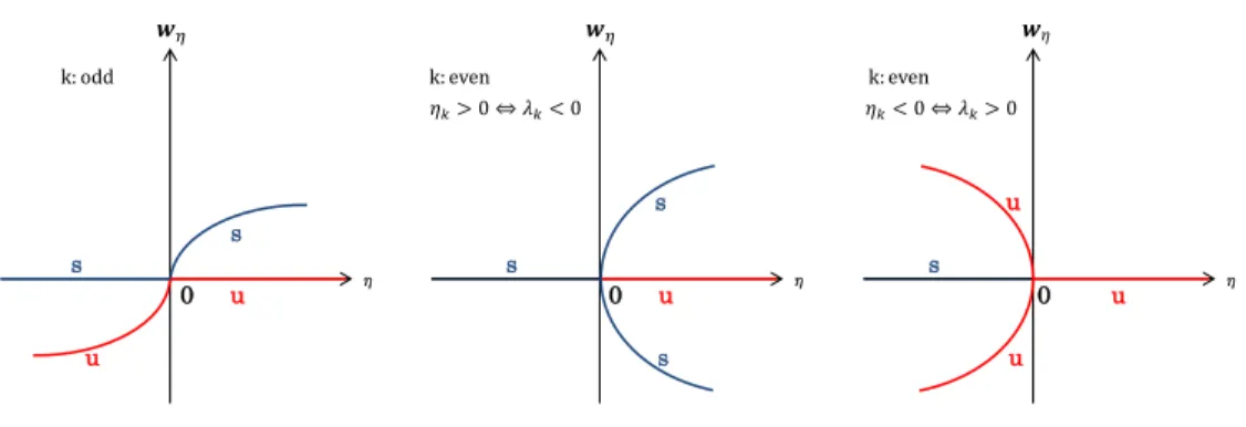
The properties of the eigenvalues of the linearized operator around bi- furcating solution near the bifurcation point is well known. Let v_η be a basic stationary solution with a bifurcation parameter η, and let Lη de- note the linearized operator around v_η for (1.1)–(1.2). We assume that ρ(−Lη) ⊃ {λ ∈ C; Reλ ≥ −˜b₀}\{λ_η} uniformly in η ∈ [−η₀, η₀] for some positive constants ˜b₀ and η₀. Here λ_η is a simple eigenvalue of −Lη and λ_η crosses the origin when η crosses 0. Then a stationary bifurcation occurs at η = 0 and there exists a nontrivial solution branch {η(δ),v(δ)˜ }, where η(δ) and ˜v(δ) are analytic in δ(0 <|δ| ≤ δ₀). We denote by L(δ) the linearized operator around ˜v(δ).

As for the spectrum of−L(δ), it holds that ρ(−L(δ))⊃ {λ∈C; Reλ≥ −3

4

˜b0}\{λ(δ)}

for 0<|δ| ≤δ₀. Here λ(δ) is analytic in δ and satisfies λ(0) = 0. Therefore, the stability of ˜v(δ) as a solution of (1.1)–(1.2) is determined by sgn(λ(δ)) the sign of λ(δ).

We denote byL(ϵ, δ) the linearized operator around ˜v(δ) for the artificial compressible system (1.3)–(1.4). We will show, by a perturbation argument, that the spectrum of −L(ϵ, δ) near the origin is given by a simple eigenvalue λ(ϵ, δ) which satisfies

λ(ϵ, δ) =c₁(ϵ², δ)λ(δ),

wherec₁(ϵ², δ) satisfiesc₁(ϵ², δ)≥ ₂¹ uniformly for 0< ϵ≤ϵ₁and 0<|δ| ≤δ₀. As a consequence, we have

sgn(λ(ϵ, δ)) = sgn(λ(δ))

for 0 < ϵ ≤ ϵ₁ and 0 < |δ| ≤ δ₀. This implies that if ˜v(δ) is unstable as a solution of (1.1)–(1.2). Then it is also unstable as a solution of (1.3)–(1.4) for 0 < ϵ ≤ ϵ₁. Furthermore, if sgn(λ(δ)) > 0 and (1.10) is satisfied with v_s = ˜v(δ) for 0<|δ| ≤δ₀, then ˜v(δ) is stable as a solution of (1.3)–(1.4) for 0< ϵ≤ϵ₁.

This thesis is organized as follows. In section 2 we introduce notations used in this thesis. In section 3 we give an improvement of the condition (1.9).

In section 3.1 we state the result about the stability criterion for stationary solutions (Theorem 3.1). We apply Theorem 3.1 to the Taylor problem in section 3.2. In section 3.3 we prove Theorem 3.1. We show that the condition (1.9) can be replaced by the condition (1.10). In section 4 we consider the stability of bifurcating stationary solutions. In section 4.1 we state the result about the stability of bifurcating stationary solutions (Theorems 4.5 and 4.6). Section 4.2 is devoted to the proofs of Theorems 4.5 and 4.6. Section5 is devoted to a derivation of a solution formula for the problem (1.13) with ψ =0.

2 Notation

We first introduce notation used in this thesis. For 1≤p≤ ∞we denote by L^p(D) the usual Lebesgue space over Dand its norm is denoted by∥ · ∥L^p(D). The mth order L² Sobolev space overD is denoted byH^m(D), and its norm is denoted by ∥ · ∥H^m(D). When D = Ω, we simply denote these norms by

∥ · ∥p, ∥ · ∥H^m. The inner product ofL²(D) is denoted by (·,·)_L²_(D), i.e., (f, g)_L²_(D)=

∫

D

f(x)g(x)dx.

Here ¯z denotes the complex conjugate of z ∈ C. When D = Ω we simply denote (·,·)_L²_(D) by (·,·). We also defined the weighted inner product⟨⟨·,·⟩⟩_ϵ by

⟨⟨u₁, u₂⟩⟩ϵ=ϵ²(p₁, p₂) + (w₁,w₂) for u_j =^⊤(p_j,w_j), j = 1,2.

We set

H₀¹(D) = theH¹(D)-closure of C₀^∞(D), H⁻¹(D) = the dual space ofH₀¹(D),

H˙¹(D) = {f ∈L²_loc(D) : ∥∇f∥L²(D) <∞}, H˙⁻¹(D) = the dual space of ˙H¹(D).

We define L²_∗(Ω) and H_∗^k(Ω) by

L²_∗(Ω) ={f ∈L²(Ω);

∫

Ω

f(x)dx= 0}, H_∗^k(Ω) =H^k(Ω)∩L²_∗(Ω) (k ≥1).

We set

L²_σ(Ω) ={v ∈L²(Ω)³; divv = 0 in Ω, v·n|∂Ω = 0}.

Here and in what follows, n denotes the unit outward normal to ∂Ω. It is known that (L²(Ω))³ =L²_σ(Ω)⊕G²(Ω), where G²(Ω) = {∇p; p∈H_∗¹(Ω)} is orthogonal complement of L²_σ(Ω).

The orthogonal projectionPfromL²(Ω)³ontoL²_σ(Ω) is called the Helmholtz projection. We set Q=I−P.

We denote the resolvent set of an operator A by ρ(A) and the spectrum of A by σ(A). Let X and Y be Banach spaces. We denote by B(X, Y) the set of bounded linear operators from X to Y.

We introduce the linearized operators for the Navier-Stokes and the cor- responding artificial compressible systems. Let u_s = ^⊤(p_s,v_s) be a smooth

stationary solution of (1.1)–(1.2), (1.5). The equations for the perturbation is then written as

divw = 0, (2.1)

∂tw−ν∆w+vs· ∇w+w· ∇vs+w· ∇w+∇p = 0. (2.2) The boundary condition is the non-slip one:

w|Ω =0. (2.3)

Applying the Helmholtz projection P we have dw

dt +Lw+P(w· ∇w) =0. (2.4) Here L is the linearized operator around v_s on L²_σ(Ω) defined by

D(L) = (H²(Ω)∩H₀¹(Ω))³∩L²_σ(Ω),

Lw=−νP∆w+P(v_s· ∇w+w· ∇v_s), (w∈D(L)).

The corresponding artificial system is written as du

dt +L_ϵu+N(u, u) = 0. (2.5) Hereu=^⊤(p,w);L_ϵ is the linearized operator aroundu_s onH_∗¹(Ω)×L²(Ω)³ defined by

D(Lϵ) = H_∗¹(Ω)×(H²(Ω)∩H₀¹(Ω))³, L_ϵ =

(0 _ϵ¹2div

∇ −ν∆ +vs· ∇+^⊤(∇vs) )

;

and N(u, u) is the nonlinear operator given byN(u, u) =^⊤(0,w· ∇w) (u=

⊤(p,w)).

3 Stability criterion for stationary solutions

In this section, we consider what kind of stationary flows can be computed by Chorin’s method and improve the stability result given in [19].

3.1 Stability criterion

We give a sufficient condition in order for a stable stationary solution of (1.1)–(1.2) to be stable as a solution of (1.3)–(1.4) for 0< ϵ≪1.

Theorem 3.1. Suppose that ρ(−L)⊃ {λ ∈ C; Reλ ≥ −b₀} for some posi- tive constant b₀. Then there exist positive constants ϵ₀, κ₀ and b₁ such that if

inf

w∈H₀¹(Ω)³,w̸=0

Re ((Qw)· ∇v_s, Qw)

∥∇Qw∥²2

≥ −κ₀, (3.1) then ρ(−L_ϵ)⊃ {λ∈C; Reλ ≥ −b₁} for all 0< ϵ≤ϵ₀.

Remark 3.2. If we consider flows an unbounded domain Ω which is trans- lation invariant in the unbounded directions of Ω such as an infinite lager and a cylindrical domain, then we can consider a stationary flow which is periodic in the unbounded directions of Ω. For definiteness, let us consider a cylindrical domain whose unbounded direction is the x₁-axis. The problem is then formulated in the basic period domain Ω_per under the periodic boundary condition in x₁. In this case, if the stationary solution v_s which is periodic in x₁ satisfies ∂_x1v_s ̸= 0, then 0 is always an eigenvalue of −L, due to the translation invariance in x₁. As in [19], one can prove the following result instead of Theorem 3.1.

Suppose that ρ(−L) ⊃ {λ ∈ C; Reλ ≥ −b₀} \ {0} for some positive constantb₀ and0is a simple eigenvalue withKer (−L) = span{∂_x1v_s}. Then there exist positive constants ϵ₀, κ₀ and b₁ such that if

inf

w∈H_0,per¹ (Ωper)³,w̸=0

Re ((Qw)· ∇v_s, Qw)

∥∇Qw∥²2

≥ −κ₀,

then ρ(−L_ϵ) ⊃ {λ ∈ C; Reλ ≥ −b₁} \ {0} for all 0 < ϵ ≤ ϵ₀ and 0 is a simple eigenvalue with Ker (−L_ϵ) = span{∂_x1u_s}. Here H_0,per¹ (Ω_per) denotes the set of allH¹ functions onΩ_per which vanish on∂Ωand satisfy the periodic boundary condition in x₁; and u_s =^⊤(p_s,v_s) with p_s being the corresponding pressure.

Remark 3.3. On can easily see from the proofs of Theorem 3.1 and [19, Theorem 3.3] that the same result also holds for the case of the Oberbeck- Boussinesq system (1.6)–(1.8).

As an application of Theorem 3.1 we will consider the Taylor problem.

3.2 Application to the Taylor problem

We consider the Navier-Stokes equation

divv = 0, (3.2)

∂_tv−ν∆v+v· ∇v+ 1

ρ_∗∇p = 0, (3.3)

in a domain Ω_R1,R2 between two concentric cylinders with radii R₁ and R₂, R₁ < R₂. In the cylindrical coordinates (r, θ, z), the domain Ω_R1,R2 is repre- sented as

Ω_R1,R2 ={(r, θ, z) : R₁ < r < R₂, θ ∈[0, 2π], z∈R}, and the velocity field v is given by

v =v^re_r+v^θe_θ+v^ze_z

with e_r = ^⊤(cosθ,sinθ,0), e_θ = ^⊤(−sinθ,cosθ,0), e_z = ^⊤(0,0,1). Here v^r, v^θ andv^z are ther, θ andz-components ofv, respectively. The inner and outer cylinders rotate with constant angular velocitiesω₁andω₂, respectively.

We assume that ω1 >0.

The boundary conditions are given by

v^r|r=R1,R2 =v^z|r=R1,R2 = 0, v^θ|r=R1 =ω₁R₁, v^θ|r=R2 =ω₂R₂. (3.4) We impose a periodic boundary condition in z, i.e.,

v, pare 2π

α_∗-periodic in z, (3.5)

where α_∗ >0 is a given wave number.

We rewrite the problem (3.2)–(3.5) in a non-dimensional form. We intro- duce the following non-dimensional variables:

x=dx,˜ v =ω₁R₁v, t˜ = d²

ν ˜t, p= ρ_∗νω1R1

d p,˜ where d=R2−R1. Then (3.2) and (3.3) are transformed into

div_x˜v˜ = 0, (3.6)

∂˜tv˜−∆_x˜v˜+Rv˜· ∇˜xv˜+∇x˜p˜ = 0, (3.7)

whereR= ^ω1R_ν^1d is the Reynolds number. The domain Ω_R1,R2 is transformed into Ω:

Ω ={(˜r,θ,˜ z) :˜ η

1−η <r <˜ 1

1−η, θ˜∈[0,2π], z˜∈R}. Here R= ^dR_ν^1ω1 is the Reynolds number; and η= ^R_R¹

2. The boundary condi- tions (3.4) and (3.5) become

˜

v^r˜|r=˜ _1−η^η ,_1−η¹ = ˜v^z˜|r=˜ _1−η^η ,_1−η¹ = 0, v˜^θ˜|r=˜ ₁₋^η_η = 1, ˜v^θ˜|˜r=_1−η¹ = ω

η, (3.8) where ω = ^ω_ω²

1, and

˜

v,p˜are 2π

α -periodic in ˜z, (3.9)

whereα >0 is a wave number. In what follows we omit the tildes ” ˜ ” in the non-dimensional quantities ˜x, ˜t, v,˜ p, and simply write them as˜ x, t, v, p.

In the cylindrical coordinates (r, θ, z) and v = v^re_r+v^θe_θ +v^ze_z, the problem (3.6)–(4.21) is written as









divv = 0,

∂_tv^r+R[(v· ∇)v^r−¹_r(v^θ)²] = −∂_rp+ (∆v^r−_r¹2v^r− _r²2∂_θv^θ),

∂_tv^θ+R[(v· ∇)v^θ+¹_rv^rv^θ] = −_r¹∂_θp+ (∆v^θ− _r¹²v^θ+_r²2∂_θv^r),

∂_tv^z+R(v· ∇)v^z = −∂_zp+ ∆v^z,

v^r|r=₁₋^η_η,₁₋¹_η =v^z|r=₁₋^η_η,₁₋¹_η = 0, v^θ|r=₁₋^η_η = 1, v^θ|r=₁₋¹_η = ω η, and

v, p are 2π

α -periodic in z.

Here divv = ¹_r∂_r(rv^r) + ¹_r∂_θv^θ + ∂_zv^z, v · ∇ = v^r∂_r + ¹_rv^θ∂_θ +v^z∂_z and

∆ = ∂_r²+¹_r∂_r+_r¹2∂_θ²+∂_z².

This problem has a stationary solution ^⊤(p_C,v_C), the Couette flow, of the form

v_C =v_C^θ(r)e_θ, v_C^θ(r) =ar+ b r, p_C =p_C(r) = R

∫ _r

{v_C^θ(s)}² s ds,

where

a= ω−η²

η(1 +η), b= η(1−ω) (1−η)(1−η²). The perturbation ^⊤(q,w) = (p−p_C,v−v_C) is governed by

divw = 0,

∂_tw−∆w+R(v_C· ∇w+w· ∇v_C) +Rw· ∇w+∇q = 0, (3.10) w|r=_1−η^η ,_1−η^η =0, (3.11) and

w, q are 2π

α -periodic in z. (3.12)

We introduce function spaces. We denote the basic period domain by Ω_α: Ω_α ={(r, θ, z) : η

1−η < r < 1

1−η, θ ∈[0,2π],−π

α < z < π α}.

The symbol C_per^∞ stands for the space of restrictions to Ω_α of functions in C^∞(Ω) which are ^2π_α-periodic inz; andC_0,per^∞ denotes the space of restrictions to Ω_α of functions in C^∞ which are ^2π_α-periodic in z and vanish near r =

η

1−η, ₁₋¹_η. We set

L²_per = the L²(Ω_α)-closure of C_0,per^∞ , H_per^k = the H^k(Ωα)-closure of C_per^∞, H_0,per¹ = the H¹(Ω_α)-closure of C_0,per^∞ .

We note that if f ∈ H_0,per¹ , then f|z=−π/α = f|z=π/α and f|_r= ^η

1−η,₁₋¹_η = 0.

The inner product of f_j ∈L²_per (j = 1,2) is denoted by (f₁, f₂) =

∫

Ωα

f₁f₂rdrdθdz,

where f denotes the complex conjugate of f. The mean value of a function f over Ω_α is denoted by⟨f⟩:

⟨f⟩= 1

|Ω_α|

∫

Ωα

f rdrdθdz.

The set of all f ∈L²_per with ⟨f⟩= 0 is denoted by L²_per,∗, i.e., L²_per,∗ ={f ∈L²_per : ⟨f⟩= 0}.

Furthermore, we set

H_per,^k _∗ =H_per^k ∩L²_per,∗.

We denote byC_0,per,σ^∞ the set of all vector fieldsv in (C_0,per^∞ )³ with divv= 0. We set

L²_per,σ = the L²(Ω_α)³-closure of C_0,per,σ^∞ .

It is known that (L²_per)³ = L²_per,σ ⊕G²_per, where G²_per = {∇p; p ∈ H_per,¹ _∗} is the orthogonal complement of L²_per,σ.

Applying the Helmholtz projection P to (3.10) we have d

dtw+LR,Cw=−RP(w· ∇w).

Here L_R,C is the linearized operator around v_C which is defined by LR,C : L²_σ,per →L²_σ,per,

D(L_R,C) = (H_per² ∩H_0,per¹ )³∩L²_σ,per,

L_R,Cw=−P∆w+RP(v_C· ∇w+w· ∇v_C) (w∈D(L_R,C)).

The corresponding artificial compressible problem are written as d

dtu+L_R,C,ϵu=−R ( 0

w· ∇w )

,

where u =^⊤(q,w) and L_R,C,ϵ is the linearized operator around the Couette flow defined by

L_R,C,ϵ : H_per,¹ _∗×(L²_per)³ →H_per,¹ _∗×(L²_per)³, D(L_R,C,ϵ) = H_per,¹ _∗×(H_per² ∩H_0,per¹ )³, L_R,C,ϵ =

(0 _ϵ¹2div

∇ −∆ +R(v_C· ∇+^⊤(∇v_C)) )

.

Since the Couette flow and Taylor vortices are axisymmetric, in what follows, we restrict the consideration to axisymmetric functions, namely, we consider vector fields v = v^re_r +v^θe_θ +v^ze_z and scalar functions q with v^r, v^θ, v^z

and q independent ofθ. For simplicity, function spaces of axisymmetric ones and the linearized operators restricted to such function spaces are denoted by the same symbols.

The instability of the Couette flow and the occurrence of the formation of Taylor vortex patterns are stated mathematically in the following way. We fix α, ω and η and assume that ω≥0.

There exists a critical number Rc > 0 such that when R < Rc, the Couette flowv_Cis asymptotically stable, whereas, whenR>Rc, the Couette flowvC becomes unstable; in other words, ifR<Rc, thenρ(−LR,C)⊃ {λ∈ C; Reλ ≥ −b₀} for some positive constant b₀ = b₀(R), whereas, if R > Rc, then σ(−L_R,C)∩ {λ ∈C; Reλ >0} ̸=∅.

When R > Rc, for each R with 0 < R − Rc ≪ 1, there exists an axisymmetric stationary solution (the Taylor vortex) v_T = v_C + ˜v_T with

∂_zv˜_T ̸= 0 which bifurcates from v_C at R = Rc supercritically. The bifur- cating solution is unique for R ∼ Rc up to translations in z. Furthermore, v_T is orbitally stable, more precisely, the linearized operator LR,T around v_T satisfies ρ(−L_R,T) ⊃ {λ; Reλ ≥ −˜b₀} \ {0} for some positive constant

˜b0 = ˜b0(R) and 0 is a simple eigenvalue due to the translation invariance in z, the eigenspace is spanned by ∂_zv_T.

The existence of the bifurcating branch of Taylor vortices v_T was shown by Velte [26], Iudovich [16], and Kirchg¨assner and Sorger [20]; and the su- percritical bifurcation of v_T and spectral properties of LR,T are shown by numerical computations for a certain range of values of α, η, ω and R when ω ≥ 0 (even when ω is slightly negative); see the book [6] by Chossat and Iooss. Hereafter we assume that the above mentioned instability of v_C, su- percritical bifurcation of v_T and the spectral properties of L_R,T hold true.

A direct computation gives Re ((Qw)·∇vC,Qw) = 0 forw=w^r(r, z)er+ w^θ(r, z)e_θ+w^z(r, z)e_z, sinceQw =∂_rϕ_r+∂_zϕ_z for such w and v_c=v_θ(r)_θ. Applying Theorem 3.1 and the instability result [19, Theorem 3.2] to L_R,C, we have the following result.

Theorem 3.4. If R < Rc, then ρ(−L_R,C,ϵ) ⊃ {λ ∈ C; Reλ ≥ −b₁} with some positive constantb₁ =b₁(R)for sufficiently smallϵ >0; and ifR >Rc, then σ(−L_R,C,ϵ)∩ {λ ∈C; Reλ >0} ̸=∅ for sufficiently small ϵ >0.

We next consider the stability of the Taylor vortexv_T. Sincev_T =v_C+ ˜v_T bifurcates from v_C at Rc, we see that ∥∇v˜_T∥_∞ → 0 as R → Rc. We then

find that

Re ((Qw)· ∇vT,Qw)

∥∇Qw∥²₂ = Re ((Qw)· ∇v˜T,Qw)

∥∇Qw∥²₂ ≥ −C∥∇v˜_T∥∞≥ −κ₀ for R, 0<R − Rc ≪1. We apply Theorem 3.1 (cf., Remark 3.2) to obtain the following result.

Theorem 3.5. If R > Rc and R − Rc ≪ 1, then ρ(−L_R,T,ϵ) ⊃ {λ ∈ C; Reλ≥ −˜b₁} \ {0} with some positive constant ˜b₁ = ˜b₁(R) for sufficiently small ϵ > 0 and 0 is a simple eigenvalue with Ker (−L_R,T,ϵ) = span{∂_zu_T}. Here u_T =^⊤(p_T,v_T) with p_T being the pressure of the Taylor vortex.

3.3 Proof of Theorem 3.1

In this section we give a proof of Theorem 3.1. We consider the resolvent problem for −L_ϵ:

λu+Lϵu=F, u=^⊤(p,w)∈D(Lϵ), (3.13) where F =^⊤(f,g)∈H_∗¹(Ω)×L²(Ω)³ is given.

For simplicity we setν = 1. The problem (3.13) is then written as ϵ²λp+ divw = ϵ²f, (3.14) λw−∆w+vs· ∇w+w· ∇vs+∇p = g, (3.15)

w|∂Ω = 0. (3.16)

Throughout this section we assume that

ρ(−L)⊃ {λ∈C; Reλ≥ −b₀} (3.17) for some positive constant b₀.

The following two propositions imply that the part of the spectrumσ(−Lϵ) near the imaginary axis can lie only in a region Imλ=O(ϵ⁻¹) under the as- sumption (3.17).

Proposition 3.6. There exist positive constants a and b such that {λ ∈ C; Reλ≥ −aϵ²|Imλ|² +b} ⊂ρ(−L_ϵ) for all 0< ϵ≤1.

Proposition 3.6 can be proved by the standard Matsumura-Nishida energy method as in the proof of [19, Proposition 6.1]. We omit the proof.