九州大学学術情報リポジトリ
Kyushu University Institutional Repository
従属観測データにおける局所漸近二次構造モデルの モデル比較
江口, 翔一
https://doi.org/10.15017/1931722
出版情報:Kyushu University, 2017, 博士(数理学), 課程博士 バージョン:
権利関係:
Model comparison for LAQ models with dependent observations
Doctoral dissertation February 14, 2018
Shoichi Eguchi
Graduate School of Mathematics, Kyushu University.
744 Motooka, Nishi-ku, Fukuoka 819-0395, Japan.
Abstract
This doctoral dissertation is based on three original papers [21], [22], and [23]. Through this thesis, we consider the Bayesian model comparison and parametric estimation of ergodic diffusion processes. Some numerical examples and real data examples are given in order to check whether the proposed method can show a good performance.
For a model-comparison purpose, we study the asymptotic behavior of the marginal quasi-log likelihood associated with a family of locally asymptotically quadratic (LAQ) statistical experiments. Our result entails a far-reaching extension of the applicable scope of the classical approximate Bayesian model comparison due to Schwarz, with frequentist-view theoretical foundation. In particular, the proposed statistics can treat possibly misspecified generalized linear models with dependent observations. Further- more, the proposed statistics can deal with both ergodic and non-ergodic stochastic process models, where the corresponding M-estimator may of multi-scaling type and the asymptotic quasi-information matrix may be random. We deduce the consistency of the multistage optimal-model selection where we select an optimal sub-model structure step by step, so that computational cost can be much reduced.
Further, we study parametric estimation of ergodic diffusions observed at high fre- quency. Different from the previous studies, we suppose that model-time scale (sam- pling stepsize) is unknown, thereby making the conventional Gaussian quasi-likelihood not directly applicable. In this situation, we construct estimators of both model pa- rameters and model-time scale in a fully explicit way and prove that they are jointly asymptotically normally distributed. The Lq-boundedness of the obtained estimator is also derived. Moreover, we propose the BIC type statistics for model selection and show its model-selection consistency.
Acknowledgements
First, I would like to express my deepest gratitude to Professor Hiroki Masuda for his valuable guidance, suggestions and encouragement. I am grateful to Professor Ryuei Nishii, Professor Yoshihiko Maesono, Associate Professor Yoshiyuki Ninomiya and As- sociate Professor Kei Hirose for their valuable comments. I also thank to my friends for their kind support during my studies. At last but not least, my gratitude goes to my family whose heartfelt assistance to my daily life.
Shoichi Eguchi February, 2018
Contents
1 Introduction 5
2 Quasi-Bayesian information criterion 8
2.1 Setup . . . 8
2.2 Bayesian model selection principle . . . 9
2.3 Quasi-Bayesian information criterion (QBIC) . . . 11
2.3.1 Stochastic expansion . . . 12
2.3.2 Convergence of the expected values . . . 16
2.4 Model selection consistency . . . 17
2.4.1 Single-scaling case . . . 17
2.4.2 Multi-scaling case: Adaptive model comparison . . . 19
2.5 Proofs . . . 22
2.5.1 Proof of Theorem 2.3.8 . . . 23
2.5.2 Proof of Theorem 2.3.15 . . . 24
2.5.3 Proof of Theorem 2.4.2 . . . 26
2.5.4 Proof of Theorem 2.4.4 . . . 27
2.5.5 Proof of Theorem 2.4.5 . . . 28
3 QBIC for Generalized linear models 29 3.1 Model setup . . . 29
3.2 Asymptotic behavior of the QMLE . . . 30
3.3 Stochastic expansion of the the marginal quasi-log likelihood . . . 36
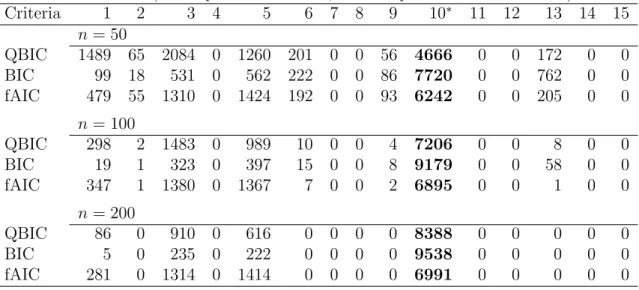
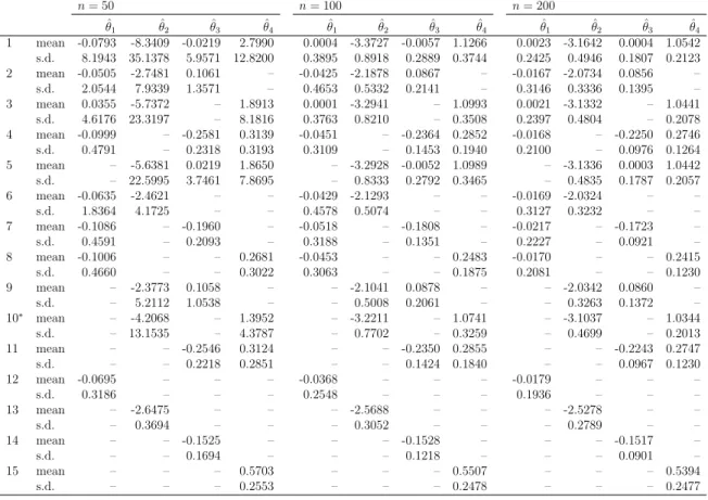
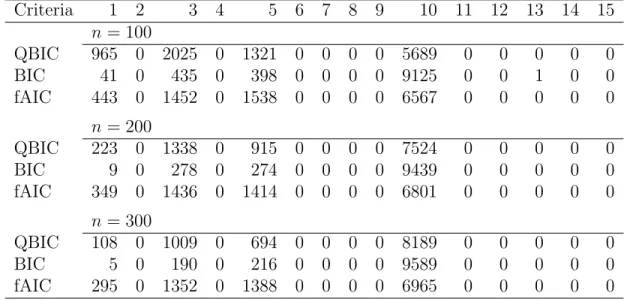
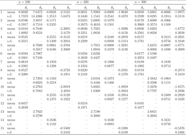
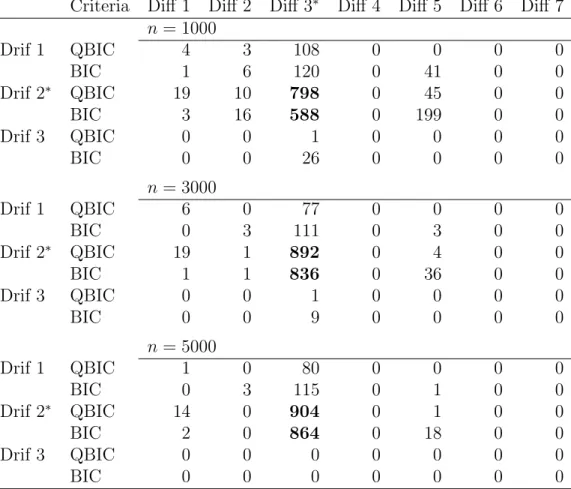
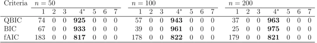
3.4 Simulation results . . . 38
3.4.1 Model selection in a correctly specified model . . . 38
3.4.2 Model selection in a misspecified model . . . 40
3.4.3 Model selection in univariate time series model . . . 41
3.5 Real data example . . . 43
3.6 Proofs . . . 46
3.6.1 Proof of Theorem 3.2.9 . . . 46
3.6.2 Proof of Theorem 3.2.11 . . . 46
3.6.3 Proof of Theorem 3.3.3 . . . 48
4 QBIC for stochastic differential equations 50
4.1 Gaussian quasi-likelihood . . . 50
4.2 Ergodic diffusion process . . . 51
4.3 Continuous semimartingale . . . 56
4.4 Simulation results . . . 57
4.4.1 Ergodic diffusion process . . . 58
4.4.2 Continuous semimartingale . . . 61
4.4.3 Non-ergodic diffusion process . . . 66
4.5 Proofs . . . 68
4.5.1 Proof of Theorem 4.2.4 . . . 68
4.5.2 Proof of Theorem 4.3.3 . . . 71
5 Data driven time scale in Gaussian quasi-likelihood inference 72 5.1 Gaussian quasi-likelihood inference with unknown time scale . . . 75
5.1.1 Setup . . . 75
5.1.2 Joint estimation . . . 75
5.1.3 Stepwise estimation . . . 82
5.1.4 Polynomial type large deviation inequality . . . 83
5.2 Consistent model selection . . . 85
5.3 Simulation experiments . . . 88
5.3.1 Parameter estimation . . . 88
5.3.2 Model selection . . . 89
5.4 Real data example . . . 95
5.5 Proofs . . . 97
5.5.1 Proof of Theorem 5.1.5 . . . 97
5.5.2 Proof of Theorem 5.1.10 . . . 107
5.5.3 Proof of Theorem 5.1.13 . . . 108 6 Implementation of model selection function in Yuima package 117
7 Appendix 121
Chapter 1 Introduction
The objective of this thesis is Bayesian model comparison for a general class of sta- tistical models, which includes various kinds of stochastic process models that cannot be handled by preceding results. There are two classical principles of model selection:
the Kullback–Leibler divergence (KL divergence) principle and the Bayesian one, acted over Akaike information criterion (AIC, [1, 2]) and Schwarz or Bayesian information criterion (BIC, [57]), respectively. A common knowledge is that there are no universal politic between AIC and BIC type statistics, and they are indeed used for different pur- poses. On the one hand, the AIC is a predictive model selection criterion minimizing the KL divergence between prediction and true models, not intended to pick up the true model consistently even if it does exist in the candidate-model set. On the other hand, the BIC is used to look for better model description, putting importance not only on underfitting but also on overfitting. The BIC usually takes the form
BICn=−2ℓn(ˆθnMLE) +plogn,
where ℓn, ˆθnMLE, and p denote the log-likelihood function, the maximum-likelihood es- timator (MLE), and the dimension of the parameter space of the statistical model to be assessed, respectively. The model selection consistency via BIC type statistics has been studied by many authors in several different model setups, for example, [8, 11], and [55], to mention just a few old ones. An extension of the BIC-derivation logic to subsume smoothly regularized likelihood estimation can be found in [41].
There also do exist many studies of the BIC methodology in the time series context.
The underlying principles, such as maximization of posterior model selection probabil- ity, remain the same in this case. It should be mentioned that [12] demonstrated that derivation of the classical BIC could be generalized into general √
n-consistent frame- work with constant asymptotic information. Their argument supposes the almost-sure behaviors of the likelihood characteristics, especially of the observed information ma- trix. Our stance is similar to theirs, but more general so as to subsume a much broader spectrum of models that cannot be handled by [12]. We note that much less has been known about theoretically guaranteed information criteria concerning sampled data
from stochastic process models; to mention some of them, we refer to [59, 60, 61, 62]
and [66].
Our primary interest is to extend the range of application of Schwarz’s BIC to a large degree in a unified way, so as to be able to target a wide class of dependent data models especially including the locally asymptotically mixed-normal family of statistical experiments. The Bayesian principle of model selection amounts choosing the model that is most likely in terms of the posterior model selection probability, which is typically measured by approximating the (expected) marginal quasi-log likelihood.
Unfortunately, a mathematically rigorous derivation of BIC type statistics is sometimes missing in the literature, especially when the underlying model is non-ergodic. In this thesis, we will focus on locally asymptotically quadratic (LAQ) statistical models. We will introduce the quasi-BIC (QBIC) through the stochastic expansion of the marginal quasi-likelihood. Here, we use the terminology “quasi” to mean that the model may be misspecified in the sense that none of candidate models may not include the true one;
see [48] for information criteria for a class of generalized linear models for independent data. Our proof of the expansion essentially utilizes the polynomial type large deviation inequality of [71]; quite importantly, the asymptotic information matrix then may be random (i.e., suitably scaled observed information (random bilinear form) has a random limit in probability), enabling us to deal with non-ergodic models in a unified way. We note the two things, though we do not go into any detail in this thesis: the popular cointegration models (see [7] and the references therein) would be in the scope of the QBIC as well; the QBIC may be closely related to the correct BIC in the context of non- stationary time series models [40], where the observed information matrix is involved in the bias-correction term. Further, it is worth mentioning that QBIC may be used even for semiparametric models, where possibly infinite-dimensional nuisance element, whenever a suitable quasi-likelihood is available.
There are many other works on the model selection, which includes the risk infor- mation criterion [27], the generalized information criterion [42], the “parametricness”
index [47], and many extensions of AIC and BIC including [15,48]. We refer to [10,16], and [43] for comprehensive accounts of information criteria, and also to [20] for an il- lustration from practical point of view.
This thesis is organized as follows. In Chapter 2, we describe some related back- grounds and present the asymptotic expansions of the marginal quasi-log likelihood (equivalently, the Bayes factor or the Kullback-Leibler divergence). We also discuss the model selection consistency with respect to the optimal model, which is naturally defined to be a minimal model among those minimizing the quasi-entropy quantities.
When in particular the quasi-maximum likelihood estimator is of multi-scaling type, we prove the consistency of the multistage optimal model selection procedure, where we partially select an optimal model structure step by step, resulting in a reduced com- putational cost. Chapter 3 presents the asymptotic properties of the quasi-maximum likelihood estimator and the BIC type statistics in possibly misspecified generalized
linear models for dependent data. In Chapter 4, we illustrate the proposed model selection method by the Gaussian quasi-likelihoods, with focuses on estimation of an ergodic diffusion process and volatility-parameter estimation for a class of continuous semimartingales, both based on high-frequency sampling; to the best of our knowledge, this is the first place that mathematically validates Schwarz’s methodology of model comparison for high-frequency data from a stochastic process. In Chapter5, we propose the modified logarithmic Gaussian quasi-likelihood and parameter estimation method and present asymptotic properties of the estimators of the model parameter and the model-time scale. We also give the sufficient conditions of the polynomial type large deviation inequality under the modified logarithmic Gaussian quasi-likelihood. Further- more, we derive the BIC type statistics in case where the model-time scale is unknown and discuss the model selection consistency with respect to the true model. Chapter 6 shows the specification of the model selection function IC in R package yuima.
We introduce some basic notations used throughout this thesis. The convergence in probability and convergence in distribution are denoted by−→P and−→L , respectively. We denote by|A| the Frobenius norm of a tensor A. If in particular, A is a square matrix, then |A| is used also for the determinant; there will be no confusion for this multiple uses. The notation′means the transpose, and the symbol ∂ak stands fork-times partial differentiation with respect to variablea. We denote byCa universal positive constant, which may change at each appearance, and write An ≲Bn if An ≤CBn a.s. for every n large enough.
Chapter 2
Quasi-Bayesian information criterion
2.1 Setup
We begin with describing our basic model setup for this thesis. Denote by X an observation random variable defined on an underlying probability space (Ω,F,P), and byGn(dx) =gn(x)µn(dx) the true distributionL(Xn), whereµnis aσ-finite dominating measure on a Borel state space ofXn, that is, Gn(dx) =P◦X−n1(dx).
Suppose that we are given a set of M candidate model M1, . . . , MM; Mm ={(
pm, πm,n(θm),Hm,n(·|θm))
|θm ∈Θm}, m = 1, . . . , M, where the ingredients in each Mm are given as follows.
• pm >0 denotes the relative likeliness of the model-Mmoccurrence amongM1, . . . , MM; we have ∑M
m=1pm = 1.
• πm,n : Θm → (0,∞) is the prior distribution L(θm) of mth-model parameter θm, here defined to be a probability density function possibly depending on the sample size n, with respect to the Lebesgue density on a bounded convex domain Θm ⊂Rpm.
• The measurable function x7→Hm,n(x|θm) for eachθm ∈Θm defines a logarithmic regular conditional probability density of L(Xn|θm) with respect to µn(dx).
EachMm may be misspecified in the sense that the true data generating model gn(x) does not belong to the family {exp{Hm,n(·|θm)}|θm ∈ Θm}; we will, however, assume suitable regularity conditions for the associated statistical random fields.
Concerning the modelMm, the random functionθm 7→exp{Hm,n(Xn|θm)}, assumed to be a.s. well-defined, is referred to as the quasi-likelihood of L(Xn|θm). The quasi- maximum likelihood estimator (QMLE) ˆθm,n associated with Hm,n is defined to be any
maximizer of Hm,n:
θˆm,n ∈argmax
θ∈Θ¯m
Hm,n(Xn|θ).
We will assume the a.s. continuity ofHm,n over the compact set ¯Θm, so that ˆθm,n always exists.
Our objective includes estimators of multi-scaling type, meaning that the compo- nents of ˆθm,n converges at different rates, which can often occur when considering high- frequency asymptotics. A typical example is the Gaussian quasi-likelihood estimation of ergodic diffusion process: see [39], also Section 4.2. Let Km ∈N be a given number, which represents the number of the components having different convergence rates in Mm, and assume that the mth-model parameter vector is divided into Km parts:
θm = (θm,1, . . . , θm,Km)∈
Km
∏
k=1
Θm,k = Θm,
with each Θm,k being a bounded convex domain inRpm,k,k ∈ {1, . . . , Km}, wherepm =
∑Km
k=1pm,k. Then, the QMLE in themth model takes the form ˆθm,n = (ˆθm,1,n, . . . ,θˆm,Km,n).
The optimal value of θm associated with Hm,n, to be precisely defined later on, is de- noted by θm,0 = (θm,1,0, . . . , θm,Km,0),θm,k,0 ∈Θm,k. The rate matrix in the model Mm
is then given in the form
Rm,n =Rm,n(θm,0) = diag(
rm,1,n(θm,0)Ipm,1, . . . , rm,Km,n(θm,0)Ipm,Km)
, (2.1.1) where Ip denotes the p-dimensional identity matrix and rm,k,n (θm,0) are deterministic positive sequences satisfying that
rm,k,n(θm,0)→0, rm,i,n(θm,0)/rm,j,n(θm,0)→0 (i < j), n → ∞. (2.1.2) The diagonality ofRm,n(θ0) is just for simplicity.
Since we are allowing not only data dependency but also the possibility of model misspecification, we may deal with a wide range of quasi-likelihoodsHm,n, even includ- ing semiparametric situations such as the Gaussian quasi-likelihood; see Section4.3for related models.
2.2 Bayesian model selection principle
The quasi-marginal distribution ofXn in themth modelMm is given by density x7→fm,n(x) :=
∫
Θm
exp{Hm,n(x|θm)}πm,n(θm)dθm.
Typical reasoning in Bayesian principle of model selection inM1, . . . ,MM is to choose the model that is most likely to occur in terms of the posterior probability, namely to choose the model maximizing
log (
fm,n(x)pm
∑M
i=1fi,n(x)pi
)
= logfm,n(x) + logpm−log ( M
∑
i=1
fi,n(x)pi )
overm= 1, . . . , M. This is equivalent to finding argmax
m≤M {logfm,n(x) + logpm}.
Then, one proceeds with suitable almost-sure (Ω ∋ ω-wise) asymptotic expansion of the logarithm of the quasi-marginal likelihood logfm,n(x) forn → ∞around a suitable estimator, a measurable function ofx=xn for each n: when√
n(ˆθm,n−θm,0) = Op(1), the resulting form may be quite often given by
logfm,n(x) + logpm ≈Hn(x|θˆm,n)−pm
2 logn+O(1) a.s. (2.2.1) This is the usual scenario of derivation of the classical-BIC type statistics; see [12] and [48] as well as [57].
We recall that the expansion (2.2.1) is also used to approximate the Bayes factor.
The logarithmic Bayes factor of Mi against Mj is defined by the (random) ratio of posterior and prior odds: lettingP(Mi|Xn) denote the posterior probability of the ith model, we have
log BFn(i, j) := logP(Mi|Xn)/P(Mj|Xn)
pi/pj = log fi,n(Xn)
fj,n(Xn). (2.2.2) The Bayes factor measures change in model selection odds betweenMi and Mj when observing Xn. We relatively prefer Mi to Mj if log BFn(i, j) > 0, and vice versa.
A selected model via the Bayes factor minimizes the total error rates compounding false-positive and false-negative probabilities, while, different from the AIC, it has no theoretical implication for predictive performance of the selected model. For a more detailed account of the philosophy of the Bayes factor, we refer to [45].
As was explained in [48], we have yet another interpretation based on the Kullback–
Leibler (KL) divergence between the true distribution gn and the mth quasi-marginal distributionfm,n:
KL(fm,n;gn) :=−
∫ (
logfm,n(x) gn(x)
)
gn(x)µn(dx)
=∫ {
loggn(x)}
gn(x)µn(dx)−∫ {
logfm,n(x)}
gn(x)µn(dx); (2.2.3)
recall that in the classical AIC methodology we instead look at KL{fm,n(·; ˆθm,n);gn} where ˆθm,n = ˆθm,n( ˜Xn) denotes the MLE in the mth correctly specified model, con- structed from an i.i.d. copy ˜Xn of Xn. Based on (2.2.3), we choose a relatively optimal one amongM1, . . . ,MM, the model index of which equals
argmin
m≤M
KL(fm,n;gn) = argmin
m≤M
∫ {logfm,n(x)}
gn(x)µn(dx).
Comparison offi,n and fj,n is equivalent to looking at the sign of KL(fj,n;gn)−KL(fi,n;gn) =
∫ log
(fi,n(x) fj,n(x)
)
gn(x)µn(dx)
=E {
log
(fi,n(Xn) fj,n(Xn)
)}
. (2.2.4)
As was noted in [48], it is important to notice that this reasoning remains valid even when any of candidate models does not coincide with the true model. We also refer to [31] for another Bayesian variable selection device based on the KL projection.
2.3 Quasi-Bayesian information criterion (QBIC)
We here focus on a single model Mm and consider the asymptotic expansion related to Hm,n. From now on, we will omit the model index “m” from the notation, simply denoting the prior density and the quasi-log likelihood byπn(θ) andHn(θ) =Hn(Xn|θ), respectively. The parameter θ∈Θ⊂Rp is graded into K parts, say
θ = (θ1, . . . , θK), θk ∈Rpk. Here we wrote p = ∑K
k=1pk. Let θ0 ∈ Θ be a constant, which will serve as the optimal parameter defined in Section 2.4. We are thinking of situations where the contrast function Hn provides an M-estimator ˆθn such that the Rn(θ0)(ˆθn−θ0) tends in distribution to a non-trivial asymptotic distribution. The rate matrix Rn(θ0) is of the form (2.1.1) satisfying (2.1.2):
Rn =Rn(θ0) = diag(
r1,n(θ0)Ip1, . . . , rK,n(θ0)IpK) ,
where positive decreasing sequences rk,n(θ0) such that rk,n−1(θ0)/r−l,n1(θ0) → 0 for k > l;
we will assume thatRn(ˆθn)−Rn(θ0)→−P 0 (see Theorem2.3.8(ii)), so that log|Rn(ˆθn)|=
∑K
k=1pklogrk,n(ˆθn). The statistical random field associated with Hn is given by Zn(u) =Zn(u;θ0) := exp{
Hn
(θ0+Rnu)
−Hn(θ0)}
, (2.3.1)
which is defined on the admissible domain Un =Un(θ0) = {
u∈Rp;θ0+Rnu∈Θ} .
The objective here is to deduce the asymptotic behavior of the marginal quasi-log likelihood function
log (∫
Θ
exp{
Hn(θ)}
πn(θ)dθ )
, and then derive an extension of the classical BIC.
2.3.1 Stochastic expansion
We begin with the stochastic expansion of the marginal quasi-log likelihood function.
Dnote by θj the jth element of θ and by Rn,ii the (i, i)th element of Rn (i.e., Rn,ii = rj,n(θ0) for some j ∈ {1, . . . , K}). We write θk = (θ1, . . . , θk) and θk = (θk, . . . , θK), with θk,0 and θk,0 in a similar manner. Let
Yk,n(θk;θk−1) =rk,n2 (θ0)(
Hn(θk−1, θk, θk+1)−Hn(θk−1, θk,0, θk+1))
and Yk,0(θk) be random function for any k ∈ {1, . . . , K}. By convention, we neglect symbols with index K+ 1 like θK+1 and ones with index 0 likeθ0.
Assumption 2.3.1. Hn(θ) is of class C3(Θ) and satisfies the following conditions:
(i) ∆n = ∆n(θ0) := Rn∂θHn(θ0) = Op(1);
(ii) Γn = Γn(θ0) := −Rn∂θ2Hn(θ0)Rn = Γ0 +op(1), and Γ0 = diag(Γ1,0, . . . ,ΓK,0) denotes the a.s. positive definite, where Γk,0 ∈ Rpk ⊗Rpk is the a.s. positive definite for all k = 1, . . . , K;
(iii) sup
θ
Rn∂θ3Hn(θ)Rn=Op(1).
Assumption 2.3.1 implicitly sets down the optimal value θ0; of course, as in the usual M-estimation theory (e.g. [67], Chapter 5) it is possible to put more specific conditions in terms of the uniform-in-θ limits of suitable scaled quasi-log likelihoods function, but we omit them. The quadratic form Γ0 is the asymptotic quasi-Fisher information matrix, which may be random. A truly random example is the volatility- parameter estimation of a continuous semimartingale (see Section 4.3). In particular, Assumption 2.3.1 leads to the LAQ approximation of logZn:
sup
u∈A
logZn(u)− (
∆n[u]−1
2Γ0[u, u])
=op(1) (2.3.2)
for each compact set A⊂Rp.
Assumption 2.3.2. For every k = 1, . . . , K−1, the following conditions are satisfied:
(i) sup
θk+1
rk,n(θ0)∂θkHn(θk,0, θk+1)=Op(1);
(ii) sup
θk+1
−rk,n2 (θ0)∂θ2
kHn(θk,0, θk+1)−Γk,0=Op(1).
Assumption 2.3.3. There exists an a.s. positive definite random matrixΣ0 ∈Rp⊗Rp such that
(∆n,Γn)→−L (Σ−01/2η,Γ0),
where η ∼Np(o, Ip) is a random variable defined on an extension of the original prob- ability space.
Assumption 2.3.4. There exists an a.s. positive random variable χ0 such that for each κ >0,
sup
θ1;|θ1−θ1,0|≥κ
Y1,0(θ1)∨ sup
θ2;|θ2−θ2,0|≥κ
Y2,0(θ2)∨ · · · ∨ sup
θK;|θK−θK,0|≥κ
YK,0(θK)≤ −χ0κ2 a.s.
Assumption 2.3.5. There exists a constant q∈(0,1) for which (r1,n(θ0))−q
sup
θ
Y1,n(θ)−Y1,0(θ1)∨(
r2,n(θ0))−q sup
θ2
Y2,n(θ2;θ1,0)−Y2,0(θ2)
∨ · · · ∨(
rK,n(θ0))−q
sup
θK
YK,n(θK;θK−1,0)−YK,0(θK)−→P 0.
Let Π(dθ) denote the prior distribution over Θ.
Assumption 2.3.6. The distribution Π admits a bounded Lebesgue density p(θ)which is continuous and positive at θ0.
Assumption 2.3.4ensures thatθk,0 is an unique maximizer of Yk,0(θk) for allk, that is,
{θk,0}= argmax
θk
Yk,0(θk), k= 1, . . . , K.
Moreover, Assumption2.3.5implies that for everyk = 1, . . . , K,Yk,n(θk,θˆk+1,n, . . . ,θˆK,n; θk−1,0)−→P Yk,0(θk) uniformly in θk.
Theorem 2.3.7. Under Assumptions 2.3.4 and 2.3.5, we have θˆn−→P θ0.
Under Assumptions2.3.4and2.3.5, we can apply the argmax theorem (see for exam- ple [67]) to the proof of the consistency of ˆθk,nsince ˆθk,n ∈argmaxθkYk,n(θk,θˆk+1,n, . . . ,θˆK,n; θˆ1,n, . . . ,θˆk−1,n). Hence, Theorem 2.3.7 is established. The next theorem shows the asymptotic expansion of the marginal quasi-log likelihood function.
Theorem 2.3.8. Suppose that Assumptions 2.3.1 to 2.3.6 are satisfied.
(i) We have the asymptotic expansion log
(∫
Θ
exp{
Hn(θ)}
πn(θ)dθ )
=Hn(θ0) +
∑K k=1
pklogrk,n(θ0) + p
2log 2π+ logπn(θ0)
− 1
2log|Γ0|+1 2Γ−01[
∆⊗n2]
+op(1).
(ii) If further logrk,n(ˆθn) = logrk,n(θ0) +op(1) for all k = 1, . . . , K, then log
(∫
Θ
exp{
Hn(θ)}
πn(θ)dθ )
=Hn(ˆθn) +
∑K k=1
pklogrk,n(ˆθn) + p
2log 2π+ logπn(ˆθn)
− 1
2log−Rn(ˆθn)∂θ2Hn(ˆθn)Rn(ˆθn)+op(1).
Remark 2.3.9. Assume that Assumptions2.3.1 and2.3.6hold and that logrk,n(ˆθn) = logrk,n(θ0) + op(1) for all k = 1, . . . , K. Theorem 2.3.8 is satisfied if the following condition hold: for anyϵ >0 there exist M > 0 andN ∈N such that
sup
n≥NP (∫
Un∩{|u|≥M}Zn(u)du > ϵ )
< ϵ. (2.3.3)
See [23] for details.
In view of Theorem2.3.8 (ii), we obtain log
(∫
Θ
exp{
Hn(θ)}
πn(θ)dθ )
=Hn(ˆθn)−1
2log−∂θ2Hn(ˆθn)+Op(1)
=Hn(ˆθn)−1 2
∑K k=1
pklogr−k,n2(ˆθn) +Op(1).
Ignoring the Op(1) parts, we define the quasi-Bayesian information criterion (QBIC) and Bayesian information criterion (BIC)by
QBICn=−2Hn(ˆθn) + log−∂θ2Hn(ˆθn), (2.3.4)
BICn=−2Hn(ˆθn) +
∑K k=1
pklogrk,n−2(ˆθn), (2.3.5) respectively. Note that in the classical case of single√
n-scaling (2.3.5) reduces to the familiar form
BICn=−2Hn(ˆθn) +plogn.
The statistics QBICn thus provides us with a far-reaching extension of derivation ma- chinery of the classical BIC. Although the QBIC (2.3.4) may have higher computa- tional load than the BIC (2.3.5), it enables us to incorporate a model-complexity bias correction taking the volume of observed information into account. In particular, to re- flect data information for dependent-data models, (2.3.4) would be more suitable than (2.3.5) whose bias correction is only based on the rate of convergence.
Let QBIC(1)n , . . . ,QBIC(Mn ) be the QBIC values in each candidate model. We com- pute QBIC(1)n , . . . ,QBIC(M)n and select the best modelMm0 in the sense of approximate Bayesian model description:
{m0}= argmin
1≤m≤M
QBIC(m)n ,
the uniqueness being implicitly assumed. The best model can be selected using the BIC in a similar manner.
Remark 2.3.10. Making use of the observed information matrix (2.3.4) for regulariza- tion has been already mentioned in the literature; for example, [8]; [38], and [58] contain such statistics for some variants of the AIC statistics. Further, it is worth mentioning that using the observed-information is a right way for some non-stationary models (see [40]).
Remark 2.3.11(Variants of QBIC). In practice, we may conveniently consider several variants of the QBIC (2.3.4). When Γ0 takes the form Γ0 = diag(Γ1,0, . . . ,ΓK,0) with each Γk,0 ∈Rpk ⊗Rpk being a.s. positive definite, we may slightly simplify the form of the QBIC as follows. We can see that under Assumption 2.3.1,
−rk,n(θ0)rl,n(θ0)∂θk∂θlHn(ˆθn) = op(1), k̸=l.
Taking logarithmic determinant of a positive definite matrix is continuous, the asymp- totic expansion in Theorem 2.3.8 (ii) becomes
log (∫
Θ
exp{
Hn(θ)}
πn(θ)dθ )
=Hn(ˆθn)− 1 2
∑K k=1
log−∂θ2
kHn(ˆθn)+Op(1), resulting in the QBIC of the form
−2Hn(ˆθn) +
∑K k=1
log−∂θ2
kHn(ˆθn). (2.3.6)
In particular, this is the case if Rn−1(ˆθn− θ0) is asymptotically mixed normally dis- tributed, with a block diagonal asymptotic (random) covariance matrix Σ0 = diag(Σ1,0, . . . ,ΣK,0) where each Σk,0 ∈Rpk ⊗Rpk is a.s. positive definite. We will deal with such an example in Section 4.2.
We may also consider finite-sample manipulations of QBIC without breaking its asymptotic behavior. For example, the problem caused by | −∂θ2Hn(ˆθn)| ≤ 0 can be avoided by using
−2Hn(ˆθn) +I{−∂θ2Hn(ˆθn)>0}
log−∂θ2Hn(ˆθn) +I{−∂θ2Hn(ˆθn)≤0}∑K
k=1
pklog(
rk,n−2(ˆθn))
instead of (2.3.4); obviously, the difference between this quantity and QBICnis ofop(1).
Further, we may useany Γˆn such that ˆΓn−→P Γ0:
−2Hn(ˆθn)−2 logRn(ˆθn)+ log|Γˆn|,
which would be convenient if ˆΓnis more likely to be stable than−Rn(ˆθn)∂θ2Hn(ˆθn)An(ˆθn);
for example, if we beforehand know the specific form of Γ0 = Γ0(θ), then it would be numerically more stable to use Γ0(ˆθn) instead of −Rn(ˆθn)∂θ2Hn(ˆθn)Rn(ˆθn).
2.3.2 Convergence of the expected values
From the frequentist point of view where Xn is regarded as a random element, it is desirable to verify the convergence of expected marginal quasi-log likelihood, which follows from the asymptotic uniform integrability of the sequence
{−2 log (∫
Θ
exp{
Hn(θ)}
πn(θ)dθ )
−QBIC♯n }
n
, where QBIC♯n =−2Hn(ˆθn) + log| −∂θ2Hn(ˆθn)| −2 logπn(ˆθn)−plog 2π.
Assumption 2.3.12. The random function Hn is of class C3(Θ) a.s. and for every r >0
sup
n E (
|∆n|r+ sup
θ
Γn(θ)r+
∑p i=1
sup
θ
Rn(θ0)∂θ3Hn(θ)Rn(θ0)r)
<∞.
Assumption 2.3.13. There exists an a.s. positive definite random matrix Γ0 such that Γn(θ0)−→P Γ0, and for some q > 3p we have
lim sup
n E(
sup
θ
λ−minq (
Γn(θ)))
<∞, where λmin(·) denotes the smallest eigenvalue of a given matrix.
The moment bounds in Assumption2.3.13was studied in [13] and [14] for some time series models, with a view toward prediction. The integrability in Assumption 2.3.13 is related to the key indexχ0 of [65] in case of volatility estimation of a continuous Itˆo process.
Under Assumptions 2.3.12 and 2.3.13, we have λ−minq (Γn(θ0)) −→P λ−minq (Γ0) by the continuous mapping theorem, and alsoλ−min1 (Γ0)∈Lq(P) as well as Γ0 ∈∩
r>0Lr(P).
Finally, we impose the boundedness of moments of the normalized estimator ˆ
un :=Rn−1(ˆθn−θ0).
Assumption 2.3.14. supnE(|uˆn|r)<∞ for somer >3.
We can now state the L1(P)-converge result.
Theorem 2.3.15. If Assumptions2.3.2to2.3.6, 2.3.12, and2.3.14hold, then we have
nlim→∞E{ −2 log
(∫
Θ
exp{
Hn(θ)}
πn(θ)dθ )
−QBIC♯n }
= 0.
In particular, QBIC♯n is an asymptotically unbiased estimator of the logarithmic quasi- marginal likelihood.
2.4 Model selection consistency
As long as concerned with good prediction performance, model selection consistency itself does not matter in an essential way. Given a set of models, it does when attempting to find the one “closest” (in the sense of KL divergence) to the true data-generating model structure itself as much as possible. For example, estimation of daily integrated volatility in econometrics would be the case, for econometricians usually builds up daily- volatility prediction model through a time series model such as, among others, ARFIMA models; an underlying continuous-time dynamics and a daily-volatility time series are separately modeled. This section is devoted to studying the validity of model selection consistency in our general setting. In particular, we propose an adaptive (stepwise) model selection strategy when we have more than one scaling rate. We start with a single-norming case, and then, before moving on to the multi-scaling case, we look at the case of ergodic diffusions since it well illustrates the proposed method.
2.4.1 Single-scaling case
We first consider cases where
rn =rm,k,n(θ0)→0
for each m ∈ {1, . . . , M} and k ∈ {1, . . . , Km}. Suppose that there exists a random functionHm,0 such that
rn2Hm,n(θm)→−P Hm,0(θm) (2.4.1) uniformly in θm ∈ Θ¯m as n → ∞ (m = 1, . . . , M). Moreover, we assume that the optimal parameter θm,0 ∈Θm in the model Mm is the unique maximizer of Hm,0:
{θm,0}= argmax
θm∈Θm
Hm,0(θm) a.s.
Ifm0 satisfies
{m0}= argmin
m∈M dim(Θm),
whereM= argmax1≤m≤MHm,0(θm,0), we say that Mm0 is the optimal model. That is, the optimal model is, if exists, an element of the optimal model set M which has the smallest dimension.
Remark 2.4.1. If we consider the correctly specified model, the optimal parameter and true parameter are equal.
Let Θi ⊂ Rpi and Θj ⊂ Rpj be the parameter space associated with Mi and Mj, respectively. We say that Θi is nested in Θj when pi < pj and there exist a matrix F ∈Rpj×pi withF′F =Ipi×pi and a constantc∈Rpj such thatHi,n(θi) = Hj,n(F θi+c) for all θi ∈ Θi. That is, when Θi is nested in Θj, any model given by a parameter in Θi can also be generated by a parameter in Θj, so that Mj includes Mi. Denote by QBIC(m)n the QBIC in Mm.
Theorem 2.4.2. Assume that (2.4.1) is satisfied and that Mm0 is the optimal model.
Let m∈ {1, . . . , M} \ {m0}, and let Assumptions 2.3.1 to 2.3.6 hold, and suppose that either
(i) Θm0 is nested in Θm, or
(ii) Hm,0(θm)̸=Hm0,0(θm0,0) a.s. for any θm ∈Θm. Then we have
nlim→∞P(
QBIC(mn 0)−QBIC(m)n <0)
= 1, (2.4.2)
nlim→∞P(
BIC(mn 0)−BIC(m)n <0)
= 1. (2.4.3)
This theorem indicates that the probability that QBIC and BIC choose the optimal model tends to 1 asn → ∞.
2.4.2 Multi-scaling case: Adaptive model comparison
For simplicity of exposition, we consider the two-scaling case, that is, K = 2. We propose a multi-step model selection procedure, which seems natural and more effective especially when an adaptive estimation procedure is possible in such a way that we can estimate a first componentθm1 without knowledge of a second one θm2. That is to say, it should be possible to select an optimal “partial” model structure associated withθm1, with regarding θm2 as a nuisance element.
We suppose that the full model is “decomposed” into two parts, each consisting of M1andM2candidates, resulting inM1×M2models in total. Write (Mm1,m2)m1≤M1;m2≤M2 for the set of all the candidate models. We are given the “full” quasi-log likelihood func- tion Hm1,m2,n(θm1, θm2). Roughly speaking, we proceed as follows.
• First, introducing an auxiliary quasi-log likelihood which is only associated with the first-component parameter θm1 and does not involve θm2, we obtain an esti- mate ˆθm1,n of θm1. Then we compare the corresponding (Q)BICs to select a first- stage optimal index, say m∗1,n ∈ {1, . . . , M1}; note that this strategy reduces the model-candidate set from{Hm1,m2,n(θm1, θm2)}m1,m2to{Hm∗1,n,m2,n(ˆθm∗
1,n,n, θm2)}m2.
• Second, based on the “partly optimized” full quasi-log likelihoods Hm∗1,n,1,n, . . . , Hm∗1,n,M2,n, we find a second-stage optimal index m∗2,n ∈ {1, . . . , M2} through (Q)BIC again.
• Finally, we pick the model Mm∗1,n,m∗2,n as our optimal model.
This adaptive procedure apparently reduces the computational cost (the number of com- parison) to much extent compared with the joint-(Q)BIC case, that is, from “O(M1× M2)” to “O(M1 +M2)”; needless to say, the amount of reduction becomes larger for K ≥3.
Remark 2.4.3. It is not essential in the above argument that the final step is based on the original quasi-log likelihood Hm1,m2,n. What is essential for the model selection consistency is that at each stage we have a suitable auxiliary quasi-likelihood function based on which we can estimate a suitably separated optimal model. We here do not go into this direction.
To be specific, we here focus on the ergodic diffusion discussed in Section 4.2, and then briefly mention the general case.
Example: Ergodic diffusion. Here we consider the same setting as in Section 4.2, that is, the model Mm1,m2 is given by (4.2.1):
dXt=am1(Xt, αm1)dwt+bm2(Xt, βm2)dt, t∈[0, Tn], X0 =x0.