The profitability effect in asset pricing model performance : an empirical study on Chinese and Japanese equity market

(1)

The profitability effect in asset pricing model performance : an empirical study on Chinese and Japanese equity market

著者（英） Dong Liu

学位名（英） Doctor of Culture and Information Science 学位授与機関（英） Doshisha University

学位授与年月日 2018‑09‑20

学位授与番号 34310甲第965号

URL http://doi.org/10.14988/di.2019.0000000177

(2)

2018 Doctoral Thesis

The profitability effect in asset pricing model performance:

An empirical study on Chinese and Japanese equity market

Graduate School of Culture and Information Science, Doshisha University

48151005 DONG LIU

Superviser Prof. Hiroshi Yadohisa

May 2018

(3)

Abstract

The question of what drives stock returns is perennial in modern finance. The Fama-French-three-factor model has been the benchmark to explain expected returns during the past two decades because the book-to-market ratio (a measure of value) and market capitalization (size) have strong explanatory power in empirical analysis. Value and size premium are always the most important factor in asset pricing model.

However, recently more and more papers question the Fama-French-three-factor model, (eg, Chen & Zhang (2010); Hou et al. (2015); Fama & French (2015)), because it has been diﬃcult to explain the cross-sectional variation in expected returns recently, especially value factor which is a redundant factor on the US market (Fama & French (2015)). People hope to find new factors that replace size and value premium.

Profitability eﬀects have attracted attention of researchers seeking to explain cross-sectional variations in stock returns. Researchers attend to profitability eﬀects because they can be used to assess the quality of firms and investment decisions.

Based on Novy-Marx (2013), gross profitability is associated with risk that cannot be captured by the value factor, the size factor. The profitability strategies belong to large growth strategies. In fact, the profitability strategy, despite generating significant returns on its own, loads strongly and negatively on the size and value factors.

Highly gross profitable firms earn higher excess returns and significantly higher abnormal returns than those with lower gross profitability firms. That reveals gross profitability have possibility to replace size and value premium.

Most of the literature is based on the US stock market and limited on the Japanese and Chinese stock market. Due to political and cultural diﬀerences, each capital

(4)

market embraces diﬀerent investment environment. Therefore, the price formation process and risk factors might be diﬀerent. Hence, we try to provide additional evidence for the literature concerning the search for a better asset pricing model.

In the chapter 3, on the Japanese market, we follow Ball et al. (2015) to investigate and compare firms’ gross profit, operating profit, and net income as predictors of returns for a cross-section of publically traded Japanese equities spanning 1994-2016. We test the predictive power of profit measures on cross-sectional stock returns using portfolio tests and Fama-MacBeth regressions, find that gross-profit- to-book-equity ratios significantly predict returns on sampled stocks. Consistent with Novy-Marx (2013), we also find that sorting portfolios by gross profitability and book-to-market ratios outperforms on the Japanese market. Hence, we create a Market-Profitability-Value model that captures value and profitability premium among returns of sampled stocks. Based on Gibbons-Ross-Shanken test and economic value, we demonstrate that our enhanced model outperforms Fama-French multiple-factor model in isolating influences on equity returns.

In the chapter 4, on the Chinese market, we follow Novy-Marx (2011, 2013) to investigate and compare firms’ gross profit, operating leverage as predictors of returns for a cross-section of traded Chinese equities spanning 1996-2016. We use portfolio tests and Fama-MacBeth regressions, find that gross-profit-to-market-capitalization ratios significantly predict returns on sampled stocks. We also find that sorting portfolios by gross profitability and size outperforms on the Chinese market. Hence, we create aMarket-Size-Profitability model that captures profitability and size premium among returns of sampled stocks. Based on Gibbons-Ross-Shanken test and economic value, we demonstrate that our enhanced model outperforms Fama-French multiple-factor model in isolating influences on equity returns.

The research contributes to the international literature on profitability eﬀect. The evidence of Japanese and Chinese stock market also provides out-of-sample tests for the existing contradicting studies which mainly focus on US market.

(5)

Chapter 1 Introduction

Chapter 1 includes a comprehensive introduction of the study. Section 1.1 describes the Research background. Section 1.2 is research problem statement. Sec- tion 1.3 explains research objectives. Section 1.4 introduces contributions of study.

Section 1.5 presents the outline of the study.

1.1 Research background

The question of whether asset prices are predictable is as central as it is old. From Harry Markowitz model (1959) to Fama-French-five-factor model (2015). Until in the AFA Annual 2018 Meeting (most famous finance distinguished meeting), still have 1/3 papers focus on the topics (see Daniel et al. (2018)). A lot of researches have been done to trace the evidence of anomaly made by the eﬀect of security returns.

People keen on researching asset pricing model, because they can put into use the evaluating mutual fund performance, measuring abnormal returns in event studies, estimating expected returns for portfolio choice, obtaining cost of equity estimates for capital budgeting, stock valuation and so on.

Fama-French-three-factor model has been popular in the last two decades, because the book-to-market ratio (value) and market capitalization (size) factors indeed have strong explanation power in empirical analysis. However, size and book-to-market ratio directly involve in market equity price information. Using price information

(9)

to explain price itself is full of controversy. Meanwhile, it is important to note that although Fama-French-three-factor models have been tested on the international markets, they show less explanatory power compared with the US evidence.

We believe that there are many anomalies affecting stock returns, and different regions have different asset pricing model to explain expected returns.

1.2 Research problem statement

There are several studies on the asset pricing impact on profitability.

Firstly, profitability has important impacts for real-world investment practices.

For example, value investors such as Benjamin Graham, Warren Buﬀett mainly attend to profitability eﬀects because they can be used to judge the quality of firms and investment decisions.

Secondly, size and value eﬀect are losing their power in many empirical researches recently, while, profitability eﬀect play important roles in generating the cross- sectional variation of expected returns. Novy-Marx (2013) shows that gross profitability is the other side of the value. Fama & French (2015), and Ball et al. (2015) reveal that profitability earns a high positive premium and helps to capture most asset-pricing anomalies that plague theFama-French-three-factor model.

Thirdly, profitability premium provides an excellent hedge for the size and value premiums and expand the investor’s investment opportunity. In addition, the forecasting power of profitability is economically and statistically strong compared to the well-known size, value and momentum eﬀects.

We research profitability eﬀect, and present a new framework that allows for multiple tests and derive recommended statistical significance levels for current research in asset pricing.

1.3 Research objective

There is ample literature focused on the profitability of stock returns especially in the developed markets. However, most of the literature is based on the US stock market and limited on the Japanese and Chinese stock markets.

(10)

China and Japan are ranked second and third, regarding GDP and stock market value in the world. The research for the two main markets are good supplement for asset pricing model theory. After all, these factors are just proved eﬀective on the US market, which is lack of persuasion. Compared to US market, Chinese and Japanese equity markets’ performance will give us more interesting stories. Meanwhile, we can also compare the diﬀerences between emerging markets and emerged markets.

1.4 Research motivation

Profitability eﬀect is widely used in US since Novy-Marx (2011,2013) and Fama &

French (2015) in the last few years. However, profitability is not directly observable, so there exists little supporting empirical evidence, especially in Japanese and Chi- nese equity markets. Hence, we try to provide additional evidence for the literature concerning the search for a better asset pricing model.

Firstly, to examine whether profitability factor is eﬀective on the Japanese and Chinese stock markets. Secondly, to examine which profitability variable is a better proxy for predicting stock returns. Thirdly, to check whether the value factor and size factor are eﬀective from the academic viewpoint. Fourthly, there is no unique factor model that explains stock returns. We try to add to profitability factor that explains stock returns well on the Japanese and Chinese market based on recent research on factor model.

1.5 Contribution of the study

The key concepts and major tasks of the dissertation are summarized as follows.

The research contributes to the international literature on profitability eﬀect. The evidence of Japanese and Chinese stock markets also provides out-of-sample tests for the existing contradicting studies which mainly focuses on US market.

Firstly, we test all kinds of profitability, operating leverage and other variables, which are not tested before on the Japanese and Chinese markets. We confirm the role of gross profitability. The research revealed gross profitability strong explained

(11)

Secondly, we are replacing the ineﬀective factors, such as book-to-market ratio (B/M) factor in China and size factor in Japan. We mirror the most famous three factor model, theFama-French-three-factor model (1993) andHou-Xue-Zhang- factor model (2015) and create local factor models on the Japanese and Chinese markets to explain returns respectively. The results prove that our enhancedMKT- GP-B/M-factor model outperforms in Japan and MKT-Size-GP-factor model outperforms in China.

Thirdly, we testified of the application of new factor model, using MSCI smart- beta index, including Large cap, Small cap, Minimum Volatility, High Dividend Yield, Risk Weighted, which can evaluate our enhanced factor model performance comprehensively. Our central contribution is to provide a new workhorse factor model for estimating expected returns.

1.6 Outline of the research

The thesis is as follows. Chapter 1 presents the introduction, the problem statement, and the motivation of the research. Chapter 2 presents an overview of the relevant literature. Chapter 3 discusses the Japanese stock market. Chapter 4 discusses the Chinese stock market. Chapter 5 summaries the major findings and implications, followed by the limitation of the research and recommendations for future research.

(12)

Chapter 2 Overview of the relevant literature

Chapter 2 includes a comprehensive theoretical and empirical literature review of the study. Section 2.1 discusses the CAPM theory. Section 2.2 reviews the evidence of factors in the prior study. Section 2.3 explains multifactor model theory. Section 2.4 introduces Japanese stock market and Chinese stock market. Section 2.5 presents the research methods used in the study. Section 2.6 explains calculation of factors.

Section 2.7 explainsGRS test. Section 2.8 provides a summary of the chapter 2.

2.1 The logic of the CAPM theory

The CAPM builds on the model of portfolio choice developed by Harry Markowitz (1959). In Markowitz’s model, investors choose “mean-variance-eﬃcient” portfolios, in the sense that the portfolios minimize the variance of portfolio return, given expected return, and maximize expected return, given variance. Thus, the Markowitz approach is often called a “mean-variance-model”. Sharpe (1965) and Lintner (1965) add two key assumptions to the Markowitz model to identify a portfolio that must be mean-variance-eﬃcient. That is The Capital Asset Pricing Model (CAPM).

The CAPM assumes that all investors have the same investing behaviour. There- fore, by aggregating utilities, a securities market line can be defined and an optimal investment portfolio can be determined. The CAPM is associated with two types of returns: risk free return of the government bonds and beta times the return on the market portfolio.

(13)

Tests of the CAPM are based on three implications of the relation between expected return and market beta implied by the model. Firstly, expected returns on all assets are linearly related to their betas, and no other variable has marginal explanatory power. Secondly, the beta premium is positive, meaning that the expected return on the market portfolio exceeds the expected return on assets whose returns are uncorrelated with the market return. Thirdly, in the Sharpe-Lintner version of the model, assets uncorrelated with the market have expected returns equal to the risk-free interest rate, and the beta premium is the expected market return minus the risk-free rate.

The formular is described as follows:

R_it−R_{f t} =α_i+β_i(R_mt−R_{f t}) +e_it. (2.1) If the markets are eﬃcient and the Sharpe-Litner version of the CAPM is the correct model, then alpha should be zero. Statistical inference to test the hypothesis α =0 is the basis of many empirical tests of the validity of the CAPM. The theory of the CAPM is that it oﬀers powerful and intuitively pleasing predictions about how to measure risk and the relation between expected return and risk.

Fama & MacBeth (1973) reveals that there is a positive cross-sectional relation between market risks and expected stock returns. The authors test the relationship between average return and risk in the New York Stock Exchange. Their result shows that the risk-return regressions are consistent with the “eﬃcient capital market”

hypothesis in which the prices of securities fully reflect the available information in the market.

However, Roll (1977) argued CAPM for two reasons. Firstly, the mean-variance eﬃciency of the market portfolio is equivalent to the CAPM equation where the stock’s unconditional α depends primarily on the covariance between its β and the market risk premium. This statement is a mathematical intuition and does not require model assumptions. Given a proxy for the market portfolio, testing the CAPM equation is equivalent to testing the mean-variance eﬃciency of the portfolio.

Secondly, the validity of the CAPM is equivalent to the market being mean-variance eﬃcient with respect to all the investment opportunities. Without looking into all

(14)

the investment opportunities, it is not possible to test whether the portfolio is mean- variance eﬃcient. Therefore, it is not possible to test the CAPM.

Unfortunately, the empirical record of the model is also poor-poor enough to invalidate the way it is used in applications. The CAPM’s empirical problems may reflect theoretical failings, the result of many simplifying assumptions.

2.2 Evidence of factors in the prior study

2.2.1 Market capitalization and value premium

Following this, many other researchers have found that the market beta alone cannot fully capture all the dimensions of risk such as the book to market eﬀect and the size eﬀect.

The size eﬀect was first tested by Banz (1981) on the US stock market and both found a return premium on small market capital stocks. The size eﬀect considers that market equity has significant marginal explanatory power on security returns.

Blume & Stambaugh (1983) confirmed the size effects using US data with the size of the bias in daily returns on stocks of small firms which is sufficient to alter the conclusions about the size effect. The biases can arise in any study that forms equally weighted rebalanced portfolios and the biases can be greatly reduced by using returns implicit in a buy and hold strategy. Moreover, Hawawini & Keim (1995) research results showed a size effect in Japan and several European markets.

Rosenberg et al. (1985) was the first who discovered a positive relationship between a return premium on the US stock markets and the high ratio of a firm’s book to market value. Since then, subsequent researchers such as Chan et al. (1991), K. Daniel & Titman (1997) have shown that the book to market eﬀect does play an important role in explaining the cross sectional variation of the Japanese stock market.

2.2.2 Momentum eﬀect

There are some other cross sectional explanatory variables used to test the rela-

(15)

tendency for rising asset prices to keep rising further and falling prices to keep falling.

Jegadeesh & Titman (1993) showed that stocks with strong past performance con- tinue to outperform stocks with poor past performance in the next period with an average excess return of about 1 % per month on US market.

Fama & French (2012) examined North America, Europe, Japan, and Asia Pacific market, indicated that the factors that lead to the momentum eﬀect in the US are not prominent in the Asian markets including Japan.

2.2.3 Profitability eﬀect

Regarding profitability eﬀect, first, we should learn about how to cause the profitability eﬀect. Inspired by valuation theory, Fama & French (2006) concludes that why these variables are related to average returns can be explained via the dividend discount model.

M_t=

∑n 1

E(D_t+n)/(1 +r)ⁿ (2.2)

The equation (2.2), M_t means market value of a share of stock, is expected dividend per share in period t+n, r is internal rate of return on dividends. Equation (2.2) says that if at timet the stocks of two firms have the same expected dividends but diﬀerent prices, the stock with a lower price has a higher expected return.

M_t =

∑n 1

E(Y_t+n−dB_t+n−1,t+n)/(1 +r)ⁿ (2.3)

The equation (2.3), D_t+n can be rewrite as Y_t+n−B_t+n₋_1,t+n,Y_t+n is total equity earnings for periodt+n, stands for expected profitability anddB_t+n =B_t+n−B_t+n₋₁ is the change in total book equity, stands fot expected investment. r is internal rate of return on dividend,stands for expected return.

The equation (2.4), dividing by time t book equity gives M_t

B_t =

∑_n

1(Y_t+n−B_t+n₋_1,t+n)/(1 +r)ⁿ

B_t (2.4)

Firstly, fix everything in (2.4) exceptB_t/M_tandr, a higher book-to-market equity

(16)

ratio, B_t/M_t, implies a higher expected return. Then fix everything in (2.4) except Y_t/B_t, will have positive relationship with the expected stock return, we callY_t/B_tas profitability. Then, fix everything in (2.4) exceptdB_t+n₋_1,t+n/B_t, will have negative relationship with the expected stock return. We call investment pattern.

Earnings in equation (2.4) represents a firm’s true economic profitability. That is theory of size, book to market ratio, profitability eﬀect and investment pattern eﬀect.

Regarding profitability premium, we consider three types of profitability, that is gross profitability, operating profitability, and net income.

Fama & French (2008) find that gross profits-to-assets has far more power than earnings. However, predicting the cross section of returns. Novy-Marx (2013) concludes that gross profit scaled by book value of total assets outperforms other measures of profitability such as earnings, cash flows, and dividends. Gross profits-to- assets is another dimension of value. They find that profitability firms measured by gross profits-to-assets (sales minus cost of goods sold and scaled by total book assets) have historically generated significantly higher returns than firms having low profitability.

Regarding the operating profitability premium, Fama & French (2015) defines the measure of operating profitability, OP, as annual revenues minus the cost of goods sold, interest expense, selling, and general and administrative expenses during the previous fiscal year divided by the end book value of equity. Operating profitability has power predicting the cross section of returns.

Ball et al. (2015) also test profitability effect, but more refining. The analysis proceeds in two stages. Firstly, they re-evaluate whether gross profitability has greater predictive power than net income, also investigate the predictive power of operating profitability. They find that operating profitability explains the cross section of expected returns better than other commonly used measures. Secondly, they compare gross profitability effect, operating profitability effect, and net income effect by same denominator, like by book value of total assets, book equity and the market value of equity.

(17)

2.3 Multifactor model theory

Except Capital Asset Pricing Model (CAPM), there are several famous multifactor models. The Fama-French-three-factor model, Carhart-four-factor model, Hou-Xue-Zhang-factor model and Fama-French-five-factor model.

Fama & French (1992) were the first to prove that market beta cannot explain the cross-sectional variation of expected returns on US stocks using the non-financial stocks traded on the New York Stock Exchange (NYSE), American Stock Exchange (AMEX), and NASDAQ during the 1963-1990 periods. Further,Fama-French-three- factor model (1993) was created.

Chen & Zhang (2010) say that the market factor, an investment factor, and a return-on-assets factor summarize the cross-sectional variation of expected stock returns. The new three-factor model substantially outperforms traditional asset pricing models in explaining anomalies associated with short-term prior returns, financial distress, net stock issues, asset growth, earnings surprises, and valuation ratios. The model’s performance, combined with its economic intuition based onq- theory, suggests that it can be used to obtain expected return estimates in practice.

The new factor model outperforms traditional asset pricing models in explaining a wide range of anomalies in the cross-section of returns.

Also inspired by q-theory, Hou et al. (2015) proposed a four-factor model which includes a market factor, size factor, investment factor and a profitability factor.

Research which applies data to test the performance of such models has shown that both models work well on the American share market.

Fama & French (2015) summarize these theories, add profitability and investment pattern to model, find that the five-factor model outperforms the three-factor model in explaining the cross section of stock returns.

(18)

2.4 Overview of the Japanese and Chinese stock markets

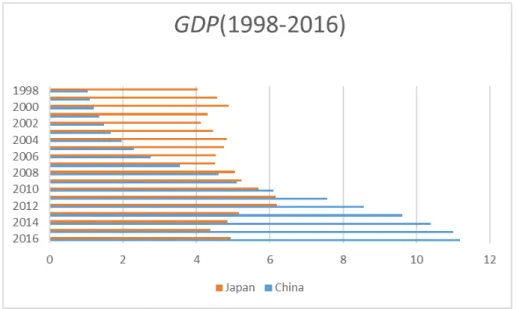
Japan is third of the world’s largest economies and one of the most important financial hubs in Asia. The Japanese GDP growth rate in Japan averaged 0.50 % from 1980 until 2017, reaching a high of 3.20 % in the second quarter of 1990 and a record low of −4.90 % in the first quarter of 2009.

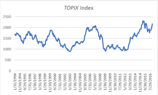
The Tokyo Stock Exchange (TSE) is the main stock exchange of the Japanese stock market. It is the world’s third largest by market capitalization. The TSE trades through two primary indexes which areNikkei 225 and theTOPIX. Currently, there are four stock exchanges operating in other Japanese cities including Osaka, Nagoya, Fukuoka and Sapporo.

Figure 2.1: The T OP IX index fluctuation (1994-2016).

After experiencing last decade’s intense reforms and development, Chinese market has increased significantly and is even comparable with that of US. The Gross Domestic Product (GDP) in China was worth 11199.15 USD Billions in 2016. The GDP value of China represents 18.06 % of the world economy. GDP in China averaged 1790.50 USD Billions from 1960 until 2016, reaching an all-time high of 11199.15 USD Billions in 2016 and a record low of 47.21 USD Billions in 1962.

Starting from ground zero in 1990, the Chinese stock market is one of the fastest

(19)

Exchanges at the end of 1990. Starting with only eight stocks listed on Shanghai and six listed on Shenzhen, the number of stocks on the two exchanges rose to 311 by the end of 1995, 720 by 1997, 1,060 by 2000 and 2,868 by 2016. Combined the two exchanges together, the total market capitalization reached 57 trillion RMB (9 trillion USD) by the end of 2017, putting China in second place globally, only after the United States (from the World Federation of Exchanges monthly report of Dec 2017), even bigger than Japan.

There are three diﬀerent types of shares in China’s stock market: A, B and H shares. A shares are dominated in renminbi (RMB) and are open mostly to domestic investors. B shares, usually dominated in U.S. dollars on the Shanghai Stock Exchange and Hong Kong dollars on the Shenzhen Stock Exchange, are mainly for foreign investors. Domestic investors are restricted from investing abroad and foreign investors are also restricted from investing in the A-share market in mainland China.

Based on Professor Robert Schiller (winner of Nobel economic award in 2013), the market is significantly underestimated when the market capitalization is below 50% or less compared to the country’s GDP scale. 50% to 75 % means somewhat underestimated, 75% to 90% means reasonable, over 90% is overvalued. From this point of view,Chinese equities are underestimated in the long term.

According to the World Bank database, China is 14.9% of global GDP, 11.7% of total exports (goods and services) and 10.0% of total imports (goods and services), but Chinese equities’ weight in theMSCI AC World Index is only 2.3%. One possible reason for such under-representation of Chinese equities may be the restrictions in market accessibility for Chinese A-shares. From this point of view, Chinese equities are under-represented in the global equity market universe relative to its economic influence.The current opening up of Chinese A-share markets allows global investors to capture China’s growth in a more direct and eﬃcient manner.

Chinese stock market has its characteristics and attract our attention. Since the number of stocks is small and the statistical information of each issue is often cut oﬀ in the middle, the maintenance of the data is incomplete. This makes the detailed analysis on the Chinese stock market diﬃcult. At the same time, on the

(20)

stock market, it is thought that there are many accounting information dressed up, there is a spread of speculative behavior, the rational institutional investors are few, and general investors in the secondary market occupy more than 70%. Because of these problems, the factors influencing the Chinese stock market may diﬀer from the Western countries and the mature markets such as Japan.

Figure 2.2: Shanghai A-share index fluctuation 1996-2016.

Figure 2.3: GDP growth rate in Japan and China 1998-2016.

(21)

2.5 Research methods used in the study

2.5.1 Single sorting

Following Novy-Marx (2013), five portfolios were formed every month, at the beginning of each month, based on profitability in order to test the relationship between the profitability and the expected stock return. All firms in the sample size were sorted based on profitability and divided equally into five groups. Portfolio 1 is the lowest fifth of all firms with the highest profitability, while portfolio 2 is the four fifth of all firms, etc. Portfolio 5 is the highest fifth of all firms with profitability. A portfolio of value weighted raw return will be computed.

2.5.2 Double sorting method

Following Fama & French (1993), the portfolios are formed to study the impact of asset pricing over the idiosyncratic risk and cross-sectional eﬀects such as size, book to market, profitability. A portfolio strategy is the most common method used in asset pricing research because it is easy to analyze and interpret the stock returns.

First of all, we sort the stocks into 5 portfolios according to its characteristics (for example: size) in the previous month at the beginning of each month. Secondly, the stocks are sorted again into 5 portfolios according to the stocks IV within each stock portfolio control variable such as size. Thirdly, 25 stock portfolios are formed which accommodate the same amount of stocks. Besides that, value-weighted portfolio raw returns for the current month were computed.

For example, by using size as the control variable, the stocks are first sorted into 5 portfolios according to the stock’s size. Therefore, the size 1 portfolio contains the first top 20 % stocks with the highest size; the size 2 portfolio contains the second top 20 % stocks, the size 3 portfolio contains the third top 20 % stocks, the size 4 portfolio contains the fourth top 20 % stocks, the size 5 portfolio contains the lowest 20 % of all stocks with low size values. After that, stocks are further sorted into 5 portfolios according to the stocks IV within each size portfolio. On the other hand, size-IV portfolios accommodate same amount of stocks. Finally, 25 portfolios were formed and can be identified as size 1-IV Low, size 1-IV 2, size 1-IV 3, size 1-IV

(22)

4, and size 1-IV-High, size 2-IV Low, size 2-IV2 and so on. This method was also appropriate for other control variables.

2.5.3 Fama-MacBeth-two-step regression

Fama & MacBeth (1973) propose a method for addressing the inference problem caused by correlation of the residuals in cross-section regressions. Instead of estimating a single cross-sectional regression of average monthly returns on beta. The Fama-MacBeth-two-step regression is a practical way of testing how these factors describe portfolio or asset returns. The goal is to find the premium from exposure to these factors. In the first step, each portfolio’s return is regressed against one or more factor time series to determine how exposed it is to each one (factor exposures).

In the second step, the cross-section of portfolio returns is regressed against the factor exposures, at each time step, to give a time series of risk premia coeﬃcients for each factor. The insight of Fama-MacBeth is to then average coeﬃcients, once for each factor, to give the premium expected for a unit exposure to each risk factor over time.

Finally, we follow the same method to explicitly test whether these variables are priced risk factor using the simple rolling cross-sectional regression methodology.

2.6 Calculation of asset pricing model

Following Fama & French (2015), we calculate the following five asset pricing factors for each region: MKT (market factor), SMB (small minus big) factor, HML (high minus low) factor, RMW (robust minus weak) factor.

Regarding of calculations of SMB, HML, RMW, we firstly classify the largest market capitalization stocks as big stocks. All remaining stocks are classified as small stocks. Then, for the region’s big stocks, we determine the usual 30 % (growth), middle 40 % (neutral), and the top 30 % (value) breakpoints for the B/M ratio and apply these breakpoints to big and small stocks. These classifications allow us to form the six value-weighted portfolios which we denote by SG, SN, SV, BG, BN, and BV where S and B refers to small and big, and G, N, and V indicate

(23)

growth, neutral, and value. SMB is the value-weighted average of the returns for the three small stock portfolios minus the average of returns for the three big stock portfolios. We construct value minus growth returns for small and big stocks,HM L_s

=SV −SG,HM L_b =BV −BG, and HML is the value-weighted average ofHM L_s and HM L_b.

The calculation of the RMW is identical to the calculation of the HML factor except that the second sort at time t is made not on the stock’s B/M ratio but on the prior year’s gross profitability. The intersection of the independent size and gross profitability sorts produces six value-weighted portfolios, SR, SN, SW, BR, BN and BW, where S and B indicate small or big, and R, N, and W indicate robust, neutral, and weak (top 30 %, middle 40 % and bottom 30 %, respectively).

We form robust minus weak returns for small and big stocks, RM W_s = SR−SW and RM W_b = BR−BW, and RMW is the value-weighted average of RM W_s and RM W_b.

2.7 GRS test

About evaluating model performance, Gibbons et al. (1989) propose the most widely used statistical test of empirical validity for asset-pricing models (GRS test).

The null hypothesis (H₀) of the GRS test is that a_i=0 jointly for all i, while the alternative hypothesis (H₁) is that at least one ai is non-zero. Under the assumption that the error term (e_i) is normally and independently distributed with zero means and nonsingular covariance matrixσ, the GRS test is a finite-sample F-test whose statistic is given by such analysis completely ignores the power of the test.

We assume that we test equation (2.1) using GRS test.The GRS Test is described as follows:

1. The GRS test is a statistical test of the hypothesis that a_i =0.

2. Equivalently, it is a test that some linear combination of the factor portfolios is on the minimum variance boundary.

3. Equivalently, it is also a test that each factor portfolio is multifactor minimum variance.

(24)

Kim & Shamsuddin (2016) consider that proportion between the maximum sharpe ratio of the three factor portfolios and the slope of the eﬃcient frontier based on all assets is an important index, which reflect ecomemic importance. Although a perfectly eﬃcient portfolio with the value of exactly and literally equal to one cannot exit in practice, the proportion the higher, the economic value is higher. We call the proportion as economic value.

In the other hand, Lewellen et al. (2010) critique the usual practice of using cross- sectional R²s and pricing errors to judge success and show that the explanatory power of many previously documented factors are spurious.

Overall, our work follow Gibbons et al. (1989), Kim & Shamsuddin (2016), and Lewellen et al. (2010), use GRS P value and economic value not cross-sectionalR², focuses on evaluating the statistical and economic significance of a factor.

2.8 Conclusion

This chapter presented the research methods used in the study which includes the single portfolios sorting, the double portfolios sorting and the Fama and Mac- beth approach. The chapter also describes overview of Japanese and Chinese stock markets. Further, this study investigates book to market ratio, momentum size and profitability eﬀect. And the detail empirical analysis will be presented in Chapter 3 and Chapter 4.

(25)

Chapter 3 Capturing profitability in asset pricing models for Japanese

equities 1994-2016

This chapter discusses the Japanese equity market. Section 3.1 describes background. Section 3.2 is literature review. Section 3.3 describes the data collection process and the definitions of the control variables used in the study. Section3.4 is empirical results. Section 3.5 discusses conclusions. Section 3.6 discusses Notes.

3.1 Introduction

Fama & French (2012), Fama & French (2017) say that Japanese market is always an exception compared to US, Europe, Asia pacific market. Like, the size premium is not so eﬀective, but value premium is stronger than other markets.

In Japan, several studies have tested asset pricing model, from three-factor model to five-factor model. Many factors own strong theory base and have been proved eﬀective on the US equity market, but not addressed on the existing literature on the Japanese equity markets. Actually, theFama-French-three-factor model on the Japanese market is the main issue about its failure to capture size premium.

Based on Novy-Marx (2013), gross profitability is associated with risk that cannot be captured by the value factor and the size factor. That gives us courage to find

(26)

the new factors, making a appropriate asset pricing model on the Japanese market.

This study tests whether the profitability predicts expected excess market returns on the Japanese equity market. Also, this study determines which profitability proxy performs best on the Japanese equity market. Our results are robust to alternative factor definitions, proxies for profitability. We confirm that gross-profit- to-book-equity is a superior proxy for predicting equity returns. Our results endorse those of Novy-Marx (2013) and support existence of a gross profitability premium for Japanese equities. In addition, we mirror Fama-French-three-factor and five- factor models, delete the redundant factor, and create a Market-Profitability-Value (MKT-RMW-HML) model to explain expected returns on Japanese equities.

3.2 Literature review

This study originates with Novy-Marx (2013), who shows that gross profitability relates significantly to equity returns after controlling for book-to-market ratio.

Profitability earns a high positive premium and helps to capture most asset-pricing anomalies that plague theFama-French-three-factor model. Fama & French (2015) add operating profitability to create a five-factor model that outperforms their three- factor model in explaining cross-sections of equity returns. Ball et al. (2015), Ball et al. (2016) present a more refined test for profitability eﬀects. Firstly, they re- evaluate whether gross profitability has greater predictive power over returns than net income and operating profitability. Secondly, they compare the eﬀects of gross profitability, operating profitability, and net income using identical denominators (book value of total assets, book equity, and market capitalization).

These literatures on the Japanese equities are as follows. Firstly, retesting Fama- French-five-factor model by examining years of monthly data for shares on the first and second sections of the Tokyo Equity Exchange(TSE), Kubota & Takehara (2018) find that operating profitability is not a statistically significant predictor of Japanese equity returns. Maeda (2017) tests q-factor (Note 1) model (market, profitability, and investment), finds that profitability (net income) is not a significant predictor of returns on Japanese equities. These studies, however, merely

(27)

retest whether an asset-pricing model is appropriate for the Japanese market. By ignoring profitability eﬀects, their conclusions lack force. This study resolves this deficiency in earlier literature. In order to provide comprehensive characterization about profitability and ensure robustness, we employ three diﬀerent measures for profitability, including gross profitability (GP), operating profitability (OP) and net income (NP). We characterize firms’ profits comprehensively using gross profit, operating profit, and net income to assure robustness in predicting equity returns.

3.3 Data and variable

Financial statement data are from the FactSet database (Note 2). Financial statements are disclosed by Japanese firms following Japanese GAAP (Generally ac- cepted accounting principles). Empirical research covers Japanese equities listed on the first section of the Tokyo Stock Exchange(TSE). Financial firms (industry codes:

7050, 7010, 7100, and 7150) are excluded for their distinctive high-leverage/low- equity capital structures. We also exclude firms with negative book value of equity to get rid of financial distressed firms. Our samples covered 834 companies in 1994, and, adjusted yearly, reached 1,658 in 2016. The observation period was from August 1994 to March 2016. We use software SAS 9.2 to do the following data processing.

We use monthly return series to measure stock return, portfolio returns, use monthly market capitalization and annual frequency data for financial statement data. For the risk free interest rate, the monthly average of the overnight call-money rate without collateral as reported by Bank of Japan.

To construct factors that might influence equity returns, we assemble annual financial statement data for sales (SALE), cost of goods sold (COGS), sales-general- administrative expenses (SGA), book value of total assets (AT), and book equity(BE) measured as AT minus total liabilities (LT). We measure investment patterns (INV) as changes in total assets (AT) every year. Log(ME) is the log of market capitalization. B/M indicates the book-to-market ratio (BE/ME). Gross profit (GP) is SALE minus COGS. Operating profit (OP) is SALE minus COGS and SGA. Bottom-line profit (NP) is net income.

(28)

GP (Gross Profitability) equals (Gross Profits)/(Book Equity or Total Assets or market value).

OP (Operating Profitability) equalls (Operating Profits)/(Book Equity or Total Assets or market value).

NP (Net income) equals (Net income)/(Book Equity or Total Assets or market value).

Log(ME) equals log (Market capitalization).

B/M equals Book Equity/Market capitalization.

INV equals (Assets(t)− Assets(t-1))/Total Assets.

3.4 Methods and empirical results

3.4.1 Fama-MacBeth univariate regressions on measures of profitability

We use monthly Fama and MacBeth regressions to examine whether profitability convincingly forecasts stock returns. The goal is to find the premium from exposure to these factors. In the first step, the cross-section of portfolio returns is regressed against the factor exposures, at each time step, rolling regression, to give a time series of risk premia coefficients for each factor. In the second step, collect all the risk premia coefficients, to average these coefficients, calculate t value.

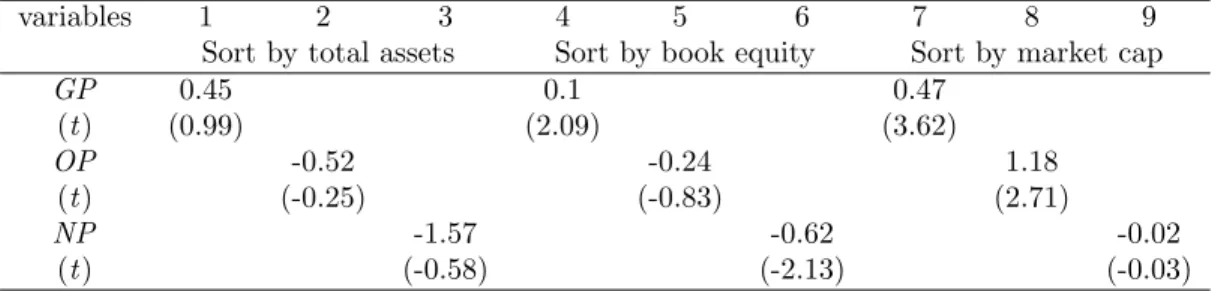
Table 3.1 shows regressed monthly returns of individual stocks on lagged profitability. We focus on t-values to compare the explanatory power of measures of profitability.

Deflating by total assets, GP, OP, and NP have no significant predicting power, while deflating by book equity,GP and NP have significant predicting power.

Deflating by market capitalization, GP and OP also have power in predicting return significant. Note, however, we admit that a market capitalization-based measure conflates a productivity proxy withB/M ratios. Hence, based on empirical tests for the sampled equities, we choose profit deflated by book equity as a proxy variable.

(29)

3.4.2 Fama-MacBeth multivariate regression

Controlling for other important determinants of stock returns. In this subsec- tion, we utilize the monthly Fama and MacBeth (1973) cross-sectional regressions to further examine the forecasting ability of profitability to predict future stock returns. We regress monthly stock returns of individual stocks on lagged profitability (measured by GP, OP and NP) for each month over 1994:08-2016:03.

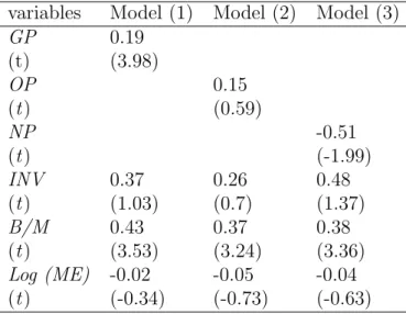
Table 3.2reports model (1)-(3) specifications for multivariate regressions including controls for book-to-market ratio (B/M), size (log(ME)), and INV (investment patterns). When controlled accordingly, the B/M is strong for the sampled equities. We reconfirm the existence of strong value eﬀects among Japanese equities per Kubota & Takehara (2007), Kubota & Takehara (2018). The size premium sheds predictive power. Investment patterns show no eﬀect on returns of sampled equities, consistent with Kubota & Takehara (2018) and unlike US equities.

GP exhibits significant power to predict returns, whereas the predictive power of OP is not significant. Results show NP has negative power to explain returns, however, motivated by valuation theory, Fama & French (2006) explore the positive relation between profitability and expected returns. Hence, we abandon net income as an investigative variable.

Based on Fama-MacBeth cross-sectional regressions, gross-profit-to-book-equity exerts the most significant power over excepted returns alone or when controlled for size, B/M, and INV. Novy-Marx (2013) concludes that gross profit is the cleanest accounting measure of true economic profitability and therefore outperforms other measures of profitability. Items farther down the income statement are more at- tenuated measures of profitability and less cogent with respect to true economic profitability.

3.4.3 Sorts on profitability

We perform portfolio tests as a more predictive exercise that escapes bias of Fama-MacBeth regressions. We compare results of gross-profit-to-book-equity, and operating-profit-to-book-equity for the sampled equities.

Specifically, at the beginning of each month, we form five deciles portfolios based

(30)

on the ranked values of profitability computed with the most recently announced annually earnings, measured by gross profitability.

Earnings data in Factset financial statements files are used in the months immedi- ately after the most recent public annually earnings announcement dates. Following Hou et al. (2015), to avoid look-ahead bias as well as ensure the accounting information of firms has been publicly known when we use it, we allow for a 5-month lag between stock returns and accounting variables.

The monthly value-weighted returns of these profitability deciles are calculated for the current month, and the portfolios are rebalanced monthly.

Particularly, decile 1 refers to firms in the lowest profitability decile, and decile 5 refers to firms in the highest profitability decile. The High-Low profitability spread portfolio is computed as long the highest profitability decile and short the lowest decile. We then compute the abnormal returns of the profitability deciles using the Fama-French-three-factor model, and examine whether standard risk factors could explain the positive profitability-return relationship. TheFama-French-three-factor model includes the market factor (MKT), the size factor (small minus big, SMB), which is the diﬀerence between the return on small and big-capitalization firms, and the value factor (high minus low, HML), which is the diﬀerence between the return on high and low book-to-market value firms. These monthly factor returns are extracted from Factset Financial Research Database.

Table 3.3documents that the monthly average abnormal returns (Fama-French- three-factor α, in percentage) of the single sorts on gross profitability, and their corresponding t-statistics (in squared brackets) from regressing the time series of excess returns of the double sorts on the Fama-French (1993) three-factors over 1994:08-2016:03 sample period.

In the GP formulation, sorting portfolios’ average excess returns are generally increasing with GP. α for the Fama-French-three-factor model increase with GP, although not monotonically. The high-minus-low quintile portfolio earns a statistically insignificant average excess return of 10 basis points per month (t-value = 0.56). Alpha for the three-factor model is 26 basis points per month (t-value = 1.41). Loading for HML is negative significant. That reveals high gross-profit-to-

(31)

book-equity portfolio generates more excess returns, meanwhile there exists negative relation between GP and B/M ratio.

In theOP formulation, in contrast with GP, the high-minus-low quintile portfolio does not spread excess returns (see Table 3.4). In fact, comparison reveals that a strategy of pursuing gross profitability generates more excess returns than pursuing operating profitability.

3.4.4 Construction of mimicking factors

We find that gross profitability is negatively correlated with book-to-market ratio.

That reveals the profitability strategy is a growth strategy, and it provides a great hedge for value strategies. We can explore the performance of portfolios double- sorted by profitability and B/M ratio to generate more excess return.

For comparison, we sort GP-B/M portfolios, OP-B/M portfolios, Size-GP portfolios, and Size-OP portfolios for the sampled equities. Average excess portfolio returns appear.

Portfolios are rebalanced monthly and formed by performing independent double sorts on book-to-market ratio and profitability. Specifically, at the beginning of each month, we independently sort firms into five B/M groups (growth to value) using the 20th, 40th, 60th, and 80thB/M percentiles and five profitability quintiles based on GP, OP. Separately, using the most recently announced annually accounting information. We compute the monthly value-weighted abnormal returns of these 25 (5*5)GP-B/M, and (5*5) OP-B/M portfolios.

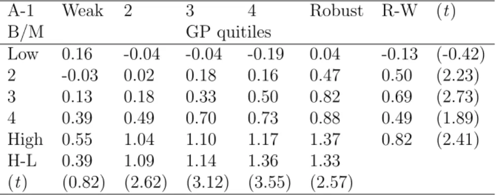
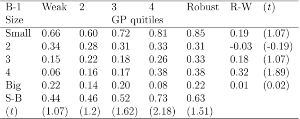
In the GP-B/M formulation in Table 3.5, except in row 1, GP and average return are positively related in all remaining rows. R-W portfolios (gross profitability premium) in rows 3 and 5 are significant. Value premium is evident in columns 2 through 5. Large value and robust profitability portfolios perform best with 1.37%

monthly returns. We confirm that controlling for GP improves performance of value strategies and controlling forB/M ratio improves performance of profitability strategies.

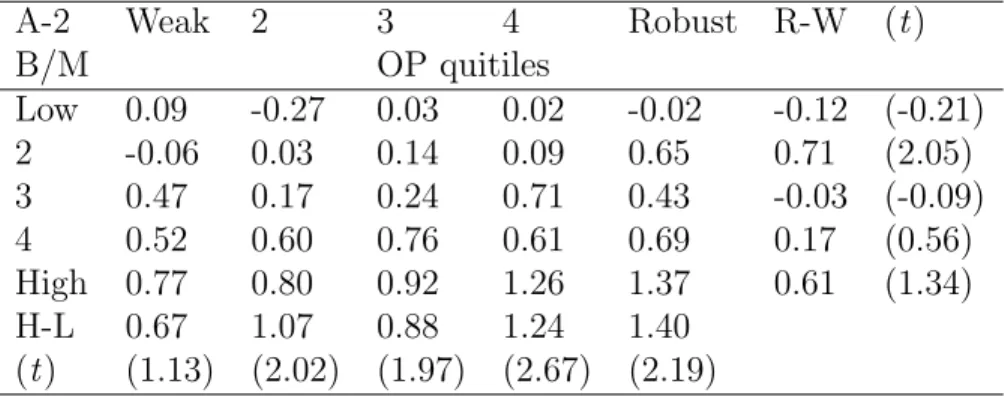
In the OP-B/M formulation in Table 3.6, the R-W portfolio (operating prof- itability premium) is positive in rows 2, 4, 5. However, only in row 2 is significant.

(32)

Value premium is eﬀective in columns 2 through 4. Overall,GP quintiles outperform OP quintiles.

Portfolios are rebalanced monthly and formed by performing independent double sorts on size and profitability. Specifically, at the beginning of each month, we independently sort firms into five size groups (small to big) using the 20th, 40th, 60th, and 80th size percentiles and five profitability quintiles based on GP, OP.

Separately, using the most recently announced annually accounting information.

We hold these portfolios for one month, and compute the monthly value-weighted abnormal returns of these 25 (5*5)Size-GP, and (5*5)Size-OP portfolios.

In the Size-GP formulation in Table 3.7, holding GP roughly constant, average return typically falls as size increases. Only the S-B portfolio (size premium) in column 4 is significant. Holding size roughly constant, average return typically increases with GP, but R-W portfolios (gross profitability premium) are not signif- icant. That finding reveals Size-GP sorting underperforms GP-B/M sorting.

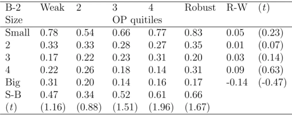
In the Size-OP formulation in Table 3.8, holding OP roughly constant, average return typically falls as size increases. Only the S-B portfolio (size premium) in column 4 is significant. Holding size roughly constant, average return typically increases with profitability. No R-W portfolio (operating profitability premium) is significant. That finding revealsSize-OP sorting underperforms OP-B/M sorting.

Overall, value quintiles outperform size quintiles. Sorting of GP and B/M portfolios outperform among the sampled equities.

3.4.5 Summary of factor model

The Fama-French-three-factor model is an empirical asset pricing model. The Fama-French-three-factor model is designed to capture the relation between average return and size and the relation between average return and price ratios like the book-to-market ratio, which were the two well-known patterns in average returns.

The model’s regression equation is

R_it−R_{f t} =α_i+β_i(R_mt−R_{f t}) +s_iSM B_t+h_iHM L_t+e_it. (3.1)

(33)

In this equation,R_it is the return on security or portfolioi for period t, R_{f t} is the risk free return, R_mt is the return on the value-weighted (VW) market portfolio of all samples,SM B_t is the return on a diversified portfolio of small stocks minus the return on a diversified portfolio of big stocks, HM L_t is the diﬀerence between the returns on diversified portfolios of high and lowB/M stocks, ande_it is a zero-mean residual. The three factor model says that the sensitivities β_i, s_i, and h_i to the portfolio returns capture all variation in expected returns, so the expected value of the intercept α_i is zero for all securities and portfoliosi.

We eliminate redundant factors to boost the model’s explanatory power. Based on Fama-MacBeth regressions and tests of combination portfolios, we define two main factor premiums: HML (high minus lowB/M) and RMW (robust minus weak GP). New factor model is

R_it−R_{f t} =α_i+β_i(R_mt−R_{f t}) +r_iRM W_t+h_iHM L_t+e_it. (3.2) In this equation, Rit is the return on security or portfolio i for period t, Rf t is the riskfree return,R_mt is the return on the value-weighted (VW) market portfolio, RM Wt is the return on a diversified portfolio of small stocks minus the return on a diversified portfolio of big stocks,HM L_t is the diﬀerence between the returns on diversified portfolios of high and low B/M stocks, and eit is a zero-mean residual.

The sensitivities β_i, r_i, and h_i to the portfolio returns capture all variation in expected returns, so the expected value of the interceptαi is zero for all securities and portfolios i.

We suggest a way to interpret the zero-intercept hypothesis, the factors are just diversified portfolios that provide different combinations of exposures to the un- known state variables. And, along with the market portfolio and the risk free asset, the factor portfolios span the relevant multifactor efficient set. In this scenario, the role of the valuation equation (2.3) is to suggest factors with risk premiums that allow us to capture the expected return effects of state variables without naming them.

To construct factor, we sort independently to assign stocks to two size groups, three B/M groups, and three profitability groups (GP). The size breakpoint is

(34)

median market cap. B/M or GP breakpoints are the 30th and 70th percentiles.

MKT (R_m−R_f) is the value-weighted return on the market portfolio of all sampled stocks minus the risk-free rate. SMB is the return on a diversified portfolio of small- cap stocks minus the return on a diversified portfolio of big-cap stocks. HML is the diﬀerence between returns on diversified portfolios of high and lowB/M stocks.

In addition, RM W_GP is the diﬀerence between returns on diversified portfolios of stocks with robust and weak gross profitability.

InTable 3.9, the 2*3 sorts used to construct RMW and HML to produce two size factors SMB, we call SM B_GP and SM B_B/M. Equivalently, we considert that SMB is the average of the returns on the six small stock portfolios minus the average of the returns on the six big stock portfolios.

3.4.6 Evaluating model performance

If a characteristic is significant in cross-sectional regressions, we hypothesized that its factor will be significant in time-series regressions. Hence, we created a new model MKT-RMW(GP)-HML model for the sampled equities and compared time-series regressions with the Fama-French-three-factor model.

About evaluating model performance, we use GRS test. Meanwhile, we follow Kim & Shamsuddin (2016), add to economic value to evaluate model performance.

About GRS test, the detail is as follows. For example, if we are testing the Fama-French-three-factor model, equation 3.1.

Step 1, we would run time series regressions for all test porofolios, like 5*5 GP- B/M portfolios.

Step 2, form the estimated intercepts into a 25*1 vector (α).

ˆ α=





 ˆ α₁

... ˆ α₂₅





 (3.3)

Step 3, calculate the residual for each regression, form the residuals into a T*N (260*25) matrix (note, T = total number of time period, N = Number of portfolios, L = Number of factors in the model ).

(35)

e_it=R_it−R_{f t}−α_i−β_i(R_mt−R_{f t})−s_iSM B_t−h_iHM L_t. (3.4) Step 4, compute an unbiased estimate of the covariance matrix of residuals, Σ = ˆˆ ε’ˆε /(T-N-1), ˆΣ is N*N martrix.

Step 5, calculate the sample means of the factor portfolios and form a L*1 vector of sample means, L stands for numbers of factors.

¯ µ=





 F¯₁

... F¯_L







Step 6, form the factor portfolio (excess) returns into a T*N matrix

F =







F₁₁ F₁₂ · · · F_1N F₂₁ F₂₂ · · · F_2N ... ... . .. ... F_T₁ F_T₂ · · · F_{T N}







Step 7, compute an unbiased estimate of the covariance matrix of the factors (the dimension of the covariance matrix is N*N).

Ω =ˆ (F −Fˆ)^′(F −Fˆ) T −1 where,

Fˆ =







Fˆ₁ Fˆ₂ · · · Fˆ_N Fˆ1 Fˆ2 · · · FˆN

... ... . .. ... Fˆ1 Fˆ2 · · · FˆN







(36)

Step 8, compute the GRS statistic.

(T N

)(T −N −L T −L−1

)[ αˆ^′Σˆ⁻¹αˆ 1 + ¯µ^′Ωˆ⁻¹µ¯

]

∼F(N, T −N −L)

where,

1. ˆα is a N *1 vector of estimated intercepts.

2. ˆΣ is an unbiased estimate of the residual covariance matrix.

3. ¯µis a L *1 vector of the factor portfoliosˇ sample means.

4. ˆΩis an unbiased estimate of the factor portfolios’ covariance matrix.

if α_i = 0, then the GRS statistic equals zero; the larger the αs are in absolute value the greater the GRS statistic will be.

The test models include aFama-French-three-factormodel and ourMKT-RMW(GP)- HMLfactor model. The test samples includeGP-B/M portfolios, OP-B/M portfolios, Size-GP portfolios, Size-OP portfolios, and Size-B/M portfolios.

Through the Table 3.10, for GRS P value, except 5*5Size-B/M sorting portfolios, our MKT-RMW(GP)-HML factor model outperforms the Fama-French-three- factor model. For economic value, our MKT-RMW(GP)-HML model always provides optimum. Overall, we show our MKT-RMW(GP)-HML model outperforms both the statistical and economic significance for the sampled equities.

3.5 Conclusion

McLean & Pontiﬀ (2016) argue that some stock market anomalies are less anomalous after being published. Repeatedly cited size and value factors naturally are less anomalous over time. That also impels us to seek new eﬀective factors and new- factor models. Our conclusions are as follows.

We find that gross profitability surpasses operating profitability and net income in power to predict returns on the sampled equities. This finding explains why Kubota

& Takehara (2018)) and Maeda (2017) say profitability is not a significant factor in the Japanese equity market: they choose a flawed proxy for profitability.

As a measure of profitability, gross-profit-to-book-equity explains the sampled cross-section of expected returns better than operating profitability and net income.

(37)

We extend Novy-Marx’s intuition about focusing on gross profitability rather than current revenue and construct a measure of gross profit with a stronger link to expected returns on Japanese equities.

Size premium for the sampled equities shed predictive power over time and become redundant. Value premium remains strong among our sampled equities. Hence, we created a newMKT-RMW(GP)-HML factor model and investigated the applicabil- ity of aFama-French-three-factor model on our sampled equities. Tests reveal that the model featuring gross profitability outperforms the Fama-French-three-factor model.

3.6 Note(s)

Note1. q-factor, based on q-theory (Tobin (1969)) predicts that investment fric- tions steepen the relation between expected returns and firm investment.

Note 2. FactSet integrates third-party data for 16,000+ active companies. It provides financial information and analytical applications to global buy and sell-side professionals. FactSet is popular among Japanese financial analysts and portfolio managers and the world’s third-largest provider of financial data behind Bloomberg and Thomson Reuters.

Note 3. We use Kim and Shamsuddin (2016) R package to do the GRS test.

Package: GRS.test.

Title: GRS Test for Portfolio Eﬃciency and Its Statistical Power . Version: 1.0.

Date: 2016-09-11.

Author: Jae H. Kim.

Description: Computational resources for test proposed by Gibbons, Ross, Shanken (1989) (DOI:10.2307/1913625).

The GRS test code will be published in Appendix B.

The profitability effect in asset pricing model performance : an empirical study on Chinese and Japanese equity market

The profitability effect in asset pricing model performance : an empirical study on Chinese and Japanese equity market

2018 Doctoral Thesis

The profitability effect in asset pricing model performance:

An empirical study on Chinese and Japanese equity market

Graduate School of Culture and Information Science, Doshisha University

48151005 DONG LIU

Superviser Prof. Hiroshi Yadohisa

May 2018

Abstract

Contents

Chapter 1 Introduction

1.1 Research background

1.2 Research problem statement

1.3 Research objective

1.4 Research motivation

1.5 Contribution of the study

1.6 Outline of the research

Chapter 2

Overview of the relevant literature

2.1 The logic of the CAPM theory

2.2 Evidence of factors in the prior study

2.2.1 Market capitalization and value premium

2.2.2 Momentum eﬀect

2.2.3 Profitability eﬀect

2.3 Multifactor model theory

2.4 Overview of the Japanese and Chinese stock markets

2.5 Research methods used in the study

2.5.1 Single sorting

2.5.2 Double sorting method

2.5.3 Fama-MacBeth-two-step regression

2.6 Calculation of asset pricing model

2.7 GRS test

2.8 Conclusion

Chapter 3

Capturing profitability in asset pricing models for Japanese

equities 1994-2016

3.1 Introduction

3.2 Literature review

3.3 Data and variable

3.4 Methods and empirical results

3.4.1 Fama-MacBeth univariate regressions on measures of profitability

3.4.2 Fama-MacBeth multivariate regression

3.4.3 Sorts on profitability

3.4.4 Construction of mimicking factors

3.4.5 Summary of factor model

3.4.6 Evaluating model performance

3.5 Conclusion

3.6 Note(s)