APPLICATION OF SMOOTHED PERTURBATION ANALYSIS TO A DISCRETE-TIME STATIONARY QUEUE

Journal of t h e Operations Research Society of J a p a n

Vol. 41, No. 1, March 1998

APPLICATION OF SMOOTHED PERTURBATION ANALYSIS TO A DISCRETE-TIME STATIONARY QUEUE

Daiji Horibe Naoto Miyoshi

Sumitorno Bank Kyoto University

(Received April 30, 1997; Revised August 25, 1997)

Abstract We investigate the sensitivity analysis for a discrete-time queueing system using perturbation

analysis. In discrete-time queues, not only the sample performance function but also the sampled event lifetimes are essentially discontinuous in some system parameter, and therefore the well-known infinitesimal perturbation analysis (IPA) technique fails to apply to even a simple single-server queue. We here apply an idea similar to the smoothed perturbation analysis for probabilistic routing problem (or equivalently, negative customer rare perturbation analysis), and under the stationarity and ergodicity assumptions, we obtain the strongly consistent estimator. Some simulation experiments demonstrate the validity of our estimator.

1. Introduction

With the development of digital information and telecommunication systems, discrete- time queueing systems have been actively studied in these days (cf. Miyazawa and Takagi eds. [22]). In this paper, we consider the sensitivity analysis for a discrete-time queue- ing system. For continuous-time discrete event stochastic systems, a variety of techniques for sensitivity estimation have been proposed and studied in this decade (see e.g. Glasser- man [12], and Rubinstein and Shapiro [25]). Among them, the infinitesimal perturbation analysis (IPA) is known as the most basic and efficient method, but in its application, it re- quires the strict condition on the continuity and differentiability of the sample performance function ([12]). To cover a broader class of performance measures and systems, smoothed perturbation analysis (SPA) has been introduced by Gong and Ho [l51 and further extended by Fu and Hu [g, 101. The likelihood ratio/score function (LRISF) method is also applicable for broader class of systems, but it is known that the variance of the estimate grows along with the run length of the simulation and hence this method requires relatively short regen- eration periods ([25]). Another powerful method is the rare perturbation analysis (RPA); the basic idea of this approach is to compare two rarely different processes, which are not

infinitesimally close when different, by considering the infinitesimal rate of change in the processes. This technique was originally developed as a kind of SPA for the derivative esti- mation with respect to the admission probability of a queue with routing control (Gong [l4]) or as a negativelphantom RPA for derivative with respect t o the rate of a Poisson arrival process (Brkmaud and Vtizquez-Abad [7]). And further developments include the virtual customer RPA (Baccelli and Bremaud [l]) and maximal coupling RPA (Brkmaud [3] and Bremaud and Massoulic? [6]). Brkmaud and Gong [4] give the unified view and the relation of these sensitivity estimation techniques (see also the recent monograph by Fu and Hu [ I l l ) .

When we try to apply the PA techniques t o discrete-time systems, we are confronted with the problem that not only the sample performance function but also the sampled event

SPA of a Discrete-Time Queue 153

lifetimes are essentially discontinuous in the continuous parameter of interest. Therefore, the IPA technique fails t o apply to even a simple single-server queue. In this paper, we treat a discrete-time single-server queue and, using an idea similar to the SPA for probabilistic routing (or equivalently, negative RPA), derive the derivative estimator for the steady-state expectation with respect to the parameter of the service time distribution. We should note that a similar problem about the continuous-time queue with two different service times is considered using structural IPA (SIPA) by Dai and Ho

[8]

and that a similar idea is also found in Kesidis et al. [16]. We proceed within the stationarity framework and, under the ergodicity assumption, obtain the strongly consistent derivative estimator. As for the PA in the stationarity and ergodicity framework, Konstantopoulos and Zazanis [17, 181 and Brkmaud and Lasgouttes [5] derive the IPA estimators for the stationary and ergodic G/G/l/oo queue using the Palm inversion formula, and Miyoshi [24] extends them to the SPA for multiclass queues. Brkmaud and G.ong [4] give the stationary SPA (RPA) formula for the probabilistic admission control problem of a GIG11 queue.

The rest of this paper is organized as follows: In the next section, the discrete-time queueing model we consider is detailed with introducing some notation, where the formula- tion is due to the Palm framework (see e.g. Baccelli and Brkmaud [2]). In Section 3, under some appropriate assumptions, we derive the derivative expression which is unbiased in the steady state, and in Section 4, we use the ergodic theorem to obtain the strongly consistent estimate. Section 5 contains some results of simulation experiments, which demonstrate the validity of our estimates. Finally, it is slightly discussed about the convergence rate of derivative estimates in Section 6.

2. Model Description

Consider a single-server queue with an unlimited buffer. Let {Tn}nEz be a sequence of arrival times of customers to the system, where each Tn takes its value on the set of integers Z . Conventionally, we assume that {Tn}neZ satisfies

lim Tn =+m.

n+±

The first property means that the arrival process is simple, that is, only one customer arrives a t a time, and the second says that there are only finite number of arrivals on a bounded interval. Let {rn}nez denote the interarrival time sequence satisfying Tn =

Tn+1

- Tn and let N be the counting measure on

(z,

23(Z)) with respect to {Tn}nezl that is,

N(A) = lA(Tn) for A 6' B(Z).

For each n E

Z,

the nth arriving customer requires the service of ~ ~ ( 0 ) in discrete-time units, where 0 is a real parameter in an interval

6

C R. We assume that service times are independent, identically distributed (i.i.d.) and independent of the arrival process. The server attends to one unit of work (if any) in a unit length of time. Let G ( - , 6) on R+ be the common distribution function of service times assumed right continuous with left limits. G ( - , 0) is piecewise constant and its discontinuities are in the set

L

C

M

= {l, 2, . . .

}.

Let g(x, 0) = G ( x , 0) - G(x-,

0)

for any X

>

0, that is the jump size of G a t X. Note that

154 D. Horibe & N. Miyoshi

independent of the parameter 0, we introduce the inverse function of

G ( - ,

0) on [O, l], as usual in the perturbation analysis literature,

Applying the sequence {Un}ne^ of independent and uniformly distributed random variables on [O, l], also independent of {Tn}nEzl the n t h service time is then given by 0 4 0 ) = G 1 ( U n , 0) and is indeed distributed according t o

G ( - ,

0). By the definition, on(0) takes its value on

L

Choosing the sample space

L!

such t h a t a sample point W =

{(Tn,

Un)}nez, we define the probability space (Q,

7, P)

independent of 0. Let

{ 1 9 , } ~ ~ ~

be the family of measurable shift operators on (f2,

3")

satisfying

and we assume t h a t the sequence

{(Tni

Un)}nez forms a discrete-time stationary marked point process, t h a t is,

We further assume that (N, P ) has a nonzero intensity A = E[N({O})] = P(To = 0) and that ( P , d.) is ergodic. We note by P O and EO the Palm probability with respect to (N, P) and the corresponding expectation. In the case of simple discrete-time point processes, it clearly follows t h a t PO(A) = P ( A

1

To

= 0) for any A C 3. Note t h a t {(rn1 Un)Jnez is compatible with {dTn}nezl that is, ( , ~ n , Un) = (70, Uo) o & , and P0 is invariant with respect t o gTn9 n E Z . Now, in order t o apply the perturbation analysis, we impose the following assumption on the service time distribution:

Assumption 1 (i) For any X G R + , G(x, 0) is differentiable and Lipschitz in 0, t h a t is, there exists

K q )

such t h a t , for any O1, G G,

(ii) Set C does not depend on the value of Q;

(iii) Let

6

= supsEe G ^ (Un, 0) for each n E Z. Then, A EO

[Q,;]

<

l .

Assumption 1(i) ensures the appropriate smoothness of the service time distribution with respect to 0, and l(ii) says that the discontinuities of G ( x , 0) are preserved from the pertur- bation in 0. Assumption l(iii) leads to the existence of the stationary and a.s. finite work process for the queue with input {(Tn,

Mna

(c.f. Loynes [20]). Since the work process with service times

{ C T : } ~ ~ ~

dominates that with

{ffn{Q)}&,

there exists the stationary and a.s. finite work process for any 0 C G. Let { w ( 0 ) } i c z be the work process in the system. Note t h a t W#) takes the value on Z+ and, as long as Wi(0)

>

0, it decreases by one time unit a t a unit of time between two successive arrivals, that is, the process {WJQ)Jiez

+

satisfies Wi(ff) = (0) - l)

+

l>Ez

on(@) l(i=Tn( for

z

E Z , where X+ = max(x, 0). Our performance measure is the functional J ( 0 ) = E [f ( ~ ~ ( f f ) ) ] , where f is a nondecreasing mapping from Z+ to R&. In the next section, we intend to derive a n unbiased estimator for the derivative d J ( 0 ) /dQ.

3. Derivation of the Estimator

In the most of the following, we focus our interest on the right-hand deriva,tive, that is, for A6 (> 0) such that 0

+

A6

E @, we estimate,

d+ J (0)

= lim

[f

(WO(0

+

4)

-

f

(Wo(0))]

A6

SPA of a Discrete-Time Queue

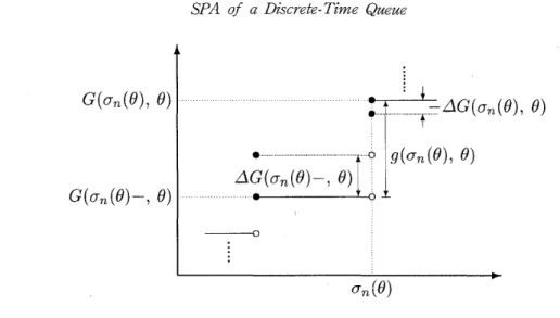
Figure 1: Change of a service time due t o a perturbation

The left-hand derivative could be derived in the similar manner. For simplicity of notation, we write

Af

(wi

(Q))

= f (Wi(Q

+

AS)) - f ( ~ ~ ( 0 ) ) for each

i

E

Z,

and similarly, for a generic function a of Q, we write Aa(0) = a(O

+

AO) - a(0). Let {Rn (Q)}nez be the sequence

of construction points a t which the arriving customers find the system empty, satisfying Ro(Q)

5

0

<

R l (0). Under the stationarity and Assumption l (iii), there are infinite number of construction points on the integer line for any 0 E

0,

and we can keep the realization of the construction points generated by {(Tn,

~ i ) } ~ ~ ~

in spite of the introduction of AO, though the additional construction points are possible, that is, noting by {R*}nEz the construction points generated by {(Tn, <7i)}nez, we have

{R*}nez

{Rn(6)}nez for any 0 E

6.

NOW, we further assume the following:

Assumption 2 (i) Let denote the work process with input {(Tn, o , " ) } ~ ~ ~ . Then, E0 [{^l

<

00.

(ii) For some 71

(>

O),

E'

[exp {71 N

([R;,

R;))

}]

<

m.

(iii) For any 6 E

G,

Kg(.) in Assumption 1(i) and for some 7~ (> O), K g ( k )

+

Kg@-)

xteLexp{72 g ^ $1

}

L 0 7 0)

<

00-

Assumption 2(ii) ensures the finiteness of any order moments of N

([R;, R'))

and (iii) also says that any order moments of { K ~ ( 0 0 (0))

+

_{( ( ( ~ ~ ( 0 )}

-)

}lg

_{(ao (S),}

Q)

_{are finite.}

In order to apply the idea of SPA, define the sub-o-field of 3'0

(=

o({A

n

{To = 0}lA E

F}))

by

Note that, on fto = {TO = O}, the process {Wi(0)}ia is (Z(Q), PO)-measurable but {Wi(Q

+

AQ)}i^i is not because we can not know whether on(0

+

AO) = an(Q) or not from the information of Z(0). Before proceeding to our main statement, we consider the conditional probability given Z(0) with which some service times change due t o the perturbation in 0. Due to the perturbation of size AQ, each value of G ( x , m ) is shifted by AG(x,

Q).

Figure 1

illustrates the change of a part of the service time distribution function. By the help of this figure, we see that the conditional probability of the event

{aJQ

+

AS)

# on

(Q)}

given on

(Q)

156 D. Horibe & N. Miyoshi

where X = - min(x, 0) and a A b = min(a, 6). In the above expression (also in Fig- ure l ) , A G ( o ~ ( Q ) ,

Q)

means A G ( x ,

Q)

1

x = (0) ~ that is, the A-operation does not work for ~

the argument on(0). We believe that no confusion arises and adopt this abuse of notation hereafter. From Assumptions 1(i) and 2(iii), when A6 is small enough, we can regard t h a t AG(on(Q), Q )

+

AG(on(0)-, 9)'

<

g ( ~ n ( ~ ) , 9) a.s., and in the rest of this paper, we consider only this case. In such a case, we can say more that

o n ( $

+

AQ) = max{k â Â : k

<

%(Q)}

1

O n ( Q ) ) = ^G ( o n (Q)

- 7 Q) +

(3.3b) g(on(Q), Q)

Since the dominant construction points {R*}nEz is preserved from the perturbation in Q, the effect to Wo(0) due t o the perturbation depends on A0 only through the change of service times of customers arriving during

[R^,

01. Let No = N ( [ R & O]), the number of customers arriving by the time origin from the beginning of the current busy period generated by {(Tn, C J : ) } ~ ~ ~ . Note t h a t , using this notation,

RE

= T-N,,+i and t h a t No is Z(0)-measurable for any Q E 6. Let

No

= {-No

+

1, . . .

,

O}. And we write for A C

No,

Then, under the independence of {Un}nEZ, we have from (3.2),

for a sufficiently small N . Now, we are a t the position to present our main statement of this section:

Theorem 1 Assume that Assumptions 1 and 2 hold. Then, J ( 0 ) =

E [ / ( w ~ ( Q ) ) ]

admits a right-hand derivative with respect to 0 given b y

where a e G ( - , 0) = 9 G ( - ,

Q)/9Q.

Also,

p

f (Wd0; n ) } = f

(w:(o;

n ) ) - f ( w i ( Q ) ) , and W*; n ) [resp. WL(0; n)] represents the value of Wi{Q) given that the service time of the nth customer is min{k E

L

: k

>

on(^)} [resp. max{k C

L

: k

<

on(Q)}] (but if on(Q) = min{k ?

L},

then W c ( 0 ; n ) = Wi(Q)).

Note t h a t each infinite summation in the right-hand side of (3.5) contains only a finite number of nonzero terms, which suggests the easy implementation of the estimator. Indeed, we have for z

>

To,

SPA of a Discrete-Time Queue

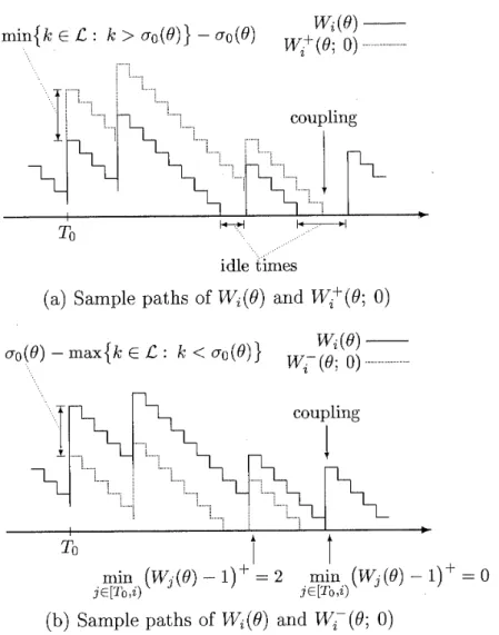
idle times

(a) Sample paths of Wi(0) and W+(Q; 0)

(b) Sample paths of Wi(0) and W;(O; 0)

Figure 2: Relation between the nominal and perturbed sample paths

b

where ~ ( [ a , b); 0) = l{wi(È)=o is the cumulative idle time from a to 6

(xi^

= 0 if b

<

a ) , and furthermore if oO(0)

#

min{k ?

L},

W; (Q; 0) = Wi

(Q)

- min (W,

(Q)

- l) + A (00

(Q)

- max{k E

L :

k

<

00

(Q)

}) ,

J€[To,

where minjEA = oo if A =

0.

Thus, both W: (0; 0) and W

(Q;

0) respectively couple to W,{Q) not later than z = R; and

/^

f ( ~ ~ ( 0 ; 0)) vanishes (see Figure 2). The inside of the expectation in (3.5) represents the conditional rate of the service time change of one customer with respect t o

Q

times the effect of such a service time change. Such a form of the estimate is common to the conditional Monte Carlo derivative estimators ([Ill). Proof: Similarly to the proofs for other perturbation analysis formulae, the key tool is the dominated convergence theorem. Applying the discrete-time version of Palm inversion formula and then characterizing by D(A0, A;

No),

we have

where the second equality follows since T>(AQ, A; N o ) ' s are pairwise disjoint. For simplicity of the notation, we write

Since

No

is (Z(O), PO)-measurable, using the conditional expectation given Z(Q)

,

where &(Q; A) represents the value of

Afa{Q)

on V{d0, A; N o )

n

Z(Q). Note that, once V(A9,

A;

No)

is given with a sufficiently small AQ, the value of

mQ;

A) no longer depends on the size of A6 since the service times of customers with indices in A change only to the possible adjacent values (see (3.3)). This is why the symbol A still remains in (3.5) even after A6 Ñ 0. Using (3.4) for sufficiently small

A6,

the inside of the expectation leads to

I -

( l -

A G ( a m ( Q ) , ( ? )

+

AG(om(Q)-,

Q)'

mdo\{n} g ( ~ m ( Q ) , Q)

In order to apply the dominated convergence theorem, we find the bounds of the three terms of the last expression of (3.6)) respectively. Using the notation of

0 - max K g ( a n (Q))

+

K g ( a n (Q)

-)

SPA of a Diswete-Time Queue

we find a bound of the first term as,

5 ~ 0 E Kg (on

(Q))

+

Kg

( o n (Q)-)

n€ g (on(0) 7

@)

T1-l

where

E

= f (W:). From the Schwarz inequality,

and the first term of the right-hand side is finite from Assumption 2(i). The same procedure leads to

and the both terms are finite from Assumption 2(ii) and (iii)? respectively. For the second and third terms of (3.6), we have

12nd term of (3.6)

1

5

lV0

E

K z ( 0 ) {l - (l - K:(Q) ~ 0 )

5

E

N~ ( N ~ - I ) K:(Q)~ ~ 0 ~ ;

No

13rd term of (3.6)

1

5

E

(T)

( K i ( 0 ) ~ 0 ) ' . 1=2

Therefore7 from Assumption 2, the expectations of the absolute values of t h third terms of (3.6) are both bounded by o(A0). Hence7 we have

e second and

Now7 applying the dominated convergence theorem and exploiting the fiTn-invariance prop- erty of PO, we have

where we use t h a t 0 E [max{R&

5

T-n}7

TWn]

implies

TPn

E [0, R;). Finally7 splitting Af-n(r3; {0}) according to (3.3) and taking the statement about infinite summation under Theorem l into account7 we obtain (3.5).

Theorem 1' Under the same assumptzons as Theorem 1, we have

Remark l When mapping f is finite, Assumption 2(i) is replaced by

(i') EO [ri]

<

CO.

When not the case, for instance? Assumption 2(i) can be replaced by (i-a) EO [rt]

<

col

(i-b) EO [f

(W;

( o ) ) ~ ]

<

CO.

Remark 2 (Monotonous

G ( - ,

0)) If the distribution function G ( . ?

Q)

is nondecreasing in Q ? then &G(.? Q)

2

0 and we have

Remark 3 (Multiple Arrival Points) In this paper, we treat only the case of a simple point process, but it would not be difficult t o extend the result to the case of multiple point processes by using the Palm probability with respect to such a process in Miyazawa and Takahashi [23].

4. Implementation of the Estimator

In this section? under the ergodicity assumptionl we derive the strongly consistent estimator for d+ J ( Q ) / d 0 based on Theorem l. The left-hand derivative version is omitted since it can be obtained in the same way.

Theorem 2 Assume that Assumptzons 1 and 2 hold. Then, under the ergodiczty of ( P l 19~)) d+ J (Q) l

= lim -

X

&G(on(Q)? 0)-

do m+m T~ n=o g ( o n ( Q ) ? 0 )

.

i2Tn

X

A+f (Wi(Q; n ) )

+

& G ( o n (Q) Q) +

P-ass, (4.1a)

g ( o n ( Q ) , Q )

Moreover, zf

G ( - ,

Q)

zs nondecreaszng zn 0) then

d+ J ( 0 ) 1 m-1 3oG(on(0)-l

Q)

= lirn -

-

A-

f (Wi(@; n ) ) P-as.

dQ m+m Tm

SPA of a Disc~ete-Time Queue 161

Proofi For simplicity7 we show equation (4.1b) only. From (3.8a)? the cross-ergodic theorem gives

d+ J(Q) 1 m-1

~ O G

(on

(Q)

- 7 Q)

do = A lim m+cx - m

X

X

A-

f

( ~ ~ ( 0 ; n)) P-ass.

n=o g(on(Q17 Q) i2Tn

On the other hand7

l m m

A = - = lim = lim - P-a.s.? E0 [TO] m+m

xr&l

Tn m+m

Tm

and the proof is completed.

Theorem 2 says that we can obtain the strongly consistent estimator for d + J ( Q ) / d Q from the single-pat h calculation (as mentioned in the previous section? each infinite summation in (4.1) contains only a finite number of nonzero terms).

5. Simulation Experiments

In order to show the validity of our estimator, we make simulation experiments for some cases. In the following examples? we take f as the identity mapping, that is7 J ( 0 ) =

EIWo(Q)]. In Example l , we treat the case where the analytical result is available7 and thus we compare the experimental results from our estimates with the analytical results. The analytical values are computed from the formula in Takagi [26]. In Example 2> we treat the case where the arrival stream has self-correlation and compare the experimental results from our estimates with the values from the symmetric finite dzflerence (FD) estimates that

are calculated by the following;

where represents the estimate from direct simulation. The F'D estimator is indeed biased but known as the last resort to obtaining the derivative estimates. We run the simulation for 807000 busy periods in each sample path and obtain the estimates with 95% confidence intervals taken from 30 independent replications. The experiments are carried out for three different values of traffic intensity p

(=

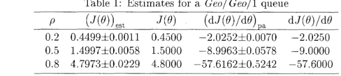
AE0[oo(Q)])7 corresponding to light traffic (p = 0.2) medium traffic ( p = 0.5) and heavy traffic ( p = 0.8) by adjusting the value of A for given Q.

Example l ( G e o / G e o / l queue) In this example, the interarrival and service times of customers are both independent and geometrically distributed with the mean l / A and l / Q 7 respectivelyl and the interarrival and service time sequences are also independent each other. The value of 0 is fixed a t 0.5. In this model7 for all n E Z 7

Table l : Estimates for a Geo/ Geo/l queue

On the other hand, in (4.1b) with

L

=

N

and f being the identity mapping7 A-Wi(Q; n) = l{minjc!Tn,i) wj ( Q I > ~ ] for on

(Q)

>

l and z

2

Tn since the service time of customer n reduces

by one time unit, and therefore, our estimate becomes

In Table l, we find t h a t our estimates have the good agreement with the analytical results.

Example 2 (TES- G e o / G e o l l queue) In this example, the service times of customers are distributed independently and geometrically as in Example l , but the interarrival times are distributed according to a correlated geometric distribution; t h a t is, using the transform expanded sample (TES) method (Melamed and Hill [21]), we generate an interarrival time sequence {rn}n20 t h a t has a marginally geometric distribution with adjacent correlation.

In this model, we adopt the T E S + ( a ,

4 )

method parameterized by 0

5

a

5

l and -1

5

4

5

l . A brief overview of this method is as follows: For any X E

B,

let [X] = max{z E Z : z

5

X} be the integral part of X , and define ( X ) = X - [X] to be the fractional part. Let

70 be a uniform random variable on 10, l ) , and a sequence {qn}n21 be of the form

where {[n}n>l - is independent and uniformly distributed sequence on [0, a ) m , and l is derived

such that

Moreover, t o remove the discontinuity of the sequence {qn}n21, transformation

S<,

parameterized by 0

<

c

<

l , of the form

Finally from St(qn) we obtain the interarrival time rn by inverting

tve introduce a smoothing

the geometric distribution function. In this simulation, we take the value a = 0.3,

4

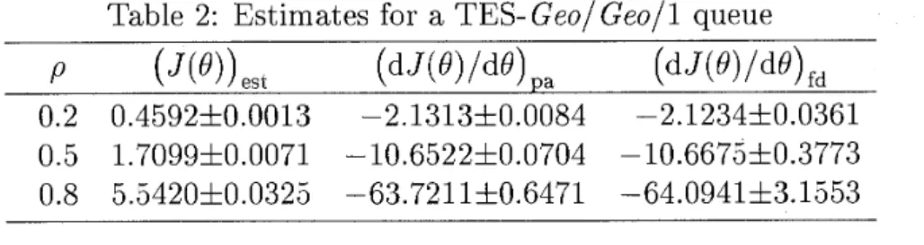
= 0.5 and = 0.5. The estimator is the same as in Example l with the fixed value of Q = 0.5, and we compare the values from our estimator with the values from FD estimator ( 5 . l ) , where A0 is taken as 0.025, 0.01 and 0.005 for p = 0.2, 0.5 and 0.8, respectively. From Table 27 we see t h a t our estimates show good agreement with FD estimates, with much smaller variance.

SPA of a Disc~ete-Time Queue

Table 2: Estimates for a TES- Geo/ Geo/l queue

6. Discussion about the Convergence Rate of Estimates

One might be interested in the asymptotic behavior of strongly consistent estimates as the observation length goes to infinity. Unfortunately7 the authors have not found any results concerning this in general case. However? in case that the system has a regenerative structure7 sorrie results have been so far obtained? where the convergence rate of estimates is often defined as the order of the square root of the mean square error with respect t o the number of regenerative cycles. Zazanis and Suri [27] show that, for the F D estimators with independent sources? one can achieve the convergence rates of 0(m-'l4) for the one- sided difference estimate and 0(m-'l3) for the symmetric difference estimate by choosing the appropriate parameter difference A0 in (5.1) as a function of m , where m denotes the number of regenerative cycles. They also show that the IPA estimate with regenerative form has the convergence rate of 0(m-'l2). For the FD estimators with common random numbers (FDC)? Glynn [l31 obtains the convergence rates of 0(m-'l3) for the one-sided case with the parameter difference A0 = rnp1I3 and 0 ( m - ~ 1 ~ ) for the symmetric case with A0 = m-1157 respectively. Also? L7Ecuyer and Perron 1191 show t h a t ? under the condition for IPA to apply, FDC has the same order of convergence rate as IPA, that is 0(m-'l2), provided that the size of the parameter difference goes t o zero fast enough.

As for our SPA estimate? if the system has the regenerative structure7 we can obtain the same convergence rate as that of the IPA estimate in the similar manner. Now7 slightly consider the general case by analogy with the regenerative case. Noting the n t h summand of (4.1a) by Pn(0) for simplicity7 the mean square error of the estimate satisfies

where the inequality holds since Tm

2

m from the simple discrete-time point process prop- erty. Since EO [!F0(0) - 7-0 d+J(O)/dO] = 0 from Theorem l, we could obtain some conver-

gence rate (not smaller than O(m-'l2)) by imposing the assumption such as the correlation in {Pn(0) - rn d + ~ ( O ) / d o } ~ ~ ~ vanishes appropriately fast? in addition to the boundedness

D. Horibe & N. Miyoshi

Acknowledgment

The authors wish t o express their sincere gratitude t o Prof. M.C. Fu, University of Maryland a t College Park, for his helpful comments on the first draft. They also thank the anonymous reviewers for useful suggestions which have made several improvements on this work. References

F. Baccelli and P. Brkmaud, "Virtual customers in sensitivity and light traffic analysis via Campbell's formula for point processes," Adv. Appl. Prob., vol. 25, pp. 221-234, 1993.

F. Baccelli and P. Brkmaud, Elements of Queueing Theory: Palm-Martingale Calculus and Stochastic Recurrences. Springer-Verlag, Berlin, 1994.

P. Brkmaud, "Maximal coupling and rare perturbation sensitivity analysis," Queueing Sys.: Theory and Appl., vol. 11, pp. 307-333, 1992.

P.

Brkmaud and W.-B. Gong, "Derivatives of likelihood ratios and smoothed pertur- bation analysis for the routing problem," ACM Trans. Modeling and Computer Simu- lation, vol. 3, pp. 134-161, 1993.

P. Brkmaud and J.-M. Lasgouttes, "Stationary IPA estimates for nonsmooth G / G / l / o o functionals via Palm inversion and level-crossing analysis," Discrete Event Dynamic Sys.: Theory and Appl., vol. 3, pp. 347-374, 1993.

P. Brkmaud and L. Massoulik, "Maximal coupling rare perturbation analysis with a random horizon," Discrete Event Dynamic Sys.: Theory and Appl., vol. 5, pp. 319- 342, 1995.

P. Brkmaud and F.J. VAzquez-Abad, "On the pathwise computation of derivatives with respect t o the rate of a point processes: The phantom RPA method," Queueing Sys.:

Theory and Appl., vol. 10, pp. 249-270, 1992.

L. Dai and Y.-C. Ho, "On derivative estimation of single-server queues via structural infinitesimal perturbation analysis," Discrete Event Dynamic Sys.: Theory and Appl., vol. 5, pp. 5-32, 1995.

M.C. Fu and J.-Q. Hu, "Extensions and generalizations of smoothed perturbation anal- ysis in a generalized semi-Markov process framework," IEEE Trans. Autom. Contr., vol. 37, pp. 1483-1500, 1992.

M.C. Fu and J.-Q. Hu, "Addendum t o 'Extensions and generalizations of smoothed perturbation analysis in a generalized semi-Markov process framework'," IEEE Trans. Autom. Contr., vol. 40, pp. 1286-1287, 1995.

M.C. Fu and J.-Q. Hu, Conditional Monte Carlo: Gradient Estimation and Optimiza- tion Applications. Kluwer Academic Publishers, Boston, 1997.

P. Glasserman, Gradient Estimation via Perturbation Analysis. Kluwer Academic Pub- lishers, Boston, 1991.

P.W. Glynn, "Optimization of stochastic systems via simulation," in Proc. of the 1989

Winter Simulation Conf., pp. 90-105, 1989.

W.-B. Gong, "Smoothed perturbation analysis algorithm for a GIG11 routing prob- lem," in Proc. of the 1988 Winter Simulation Conf., pp. 525-531, 1988.

W.-B. Gong and Y.-C. Ho, "Smoothed (conditional) perturbation analysis of discrete- event dynamic systems," IEEEE Trans. Autom. Contr., vol. 32, pp. 858-867, 1987.

SPA of a Disc~ete-Time Queue 165

[l61

G.

Kesidis, T . Konstantopou1os, and M .A. Zazanis, "Sensitivity analysis for discrete- time randomized service priority queues," in Proc. of the 33rd

IEEE

Conference on Decision and Control, pp. 2627-2630, 1994.

[l71 P. Konstantopoulos and M.A. Zazanis, "Sensitivity analysis for stationary and ergodic queues7" Adv. Appl. Prob., vol. 24, pp. 738-750, 1992.

[l81 P. Konstantopoulos and M. A. Zazanis, "Sensitivity analysis for stationary and ergodic queues: Additional results,'' Adv. Appl. Prob., vol. 2G7 pp. 556-560, 1994.

[l91 P. L7Ecuyer and

G.

Perron, "On the convergence rates of IPA and F'DC derivative estimators," Operat. Res., vol. 42, pp. 643-656, 1994.

[20] R.M. Loynes, "The stability of queues with non-independent inter-arrival and service times," Proc. of Cambridge Phil. Soc., vol. 58, pp. 497-5207 1962.

[21] B. Melamed and J.R. Hill, "A survey of TES modeling a p ~ l i c a t i o n ~ ' ~ Simulation, vol. 64, pp. 353-370, 1995.

[22] M. Miyazawa and H. Takagi, eds., Special Issue on Advances in Discrete Time Queues, Queueing Sys.: Theory and Appl., vol. 18, nos. l, 2, 1994.

[23] M. Miyazawa and Y. Takahashi, "Rate conservation principle for discrete-time queues," Queueing Sys.: Theory and Appl., vol. 12, pp. 215-230, 1992.

[24] N. Miyoshi, L'Smoothed perturbation analysis for stationary single-server queues with multiple customer classes7" Discrete Event Dynamic Sys.: Theory and Appl., vol. 7, pp. 275-293, 1997.

'

[25] R.Y. Rubinstein and A. Shapiro, Discrete Event Systems: Sensitivitg Analysis and Stochastic Optimization by the Score Function Method. John Wiley &L Sons, Chichester,

1993.

[26] H. Takagi, Queueing Analysis: A Foundation of Performance Evuluation Volume 3, Discrete- Tzme Systems. North-Holland, Amsterdam, 1993.

[27] M.A. Zazanis and

R.

Suri, "Convergence rates of finite-difference sensitivity estimates for stochastic systems," Operat. Res., vol. 41, pp. ,694-703, 1993.

Daiji HORIBE:

Koraibashi Branch, Sumitomo Bank Chuo-ku, Osaka 541, Japan

Naoto MIYOSHI:

Department of Applied Systems Science Graduate School of Engineering

Kyoto University, Kyoto 606-01, Japan E-mail: miyoshi~kuamp.kyoto-u.ac.jp