Computation of Upper and Lower Bounds of <i>L</i><sub>2</sub> Error of Multiview Triangulation Using Linear Matrix Inequalities

全文

(1)Vol.2016-CVIM-201 No.1 2016/3/3. IPSJ SIG Technical Report. Computation of Upper and Lower Bounds of L2 Error of Multiview Triangulation Using Linear Matrix Inequalities Zhenjiao Wang1,a). Yoshimichi Ito2,b). Noboru Babaguchi1,c). Abstract: This paper proposes several methods for computing upper and lower bounds of L2 error of multiview tri-. angulation. The multiview triangulation is to find the point that minimizes the sum of reprojection errors calculated by points on the image plane observed by multiple cameras. We first show the L2 optimization for multiview triangulation is reduced to the ones with nonconvex matrix inequality constraints, which are hard to solve. By relaxing the nonconvex matrix inequality constraints, we derive conditions for computing lower bounds of L2 optimal error. The conditions are represented by linear matrix inequalities (LMI), and they are easy to solve. On the other hand, by tightening the nonconvex matrix inequality constraints, we derive conditions for computing upper bounds of L2 optimal error, which are also represented by LMI. These methods are easily implemented by MATLAB using tools for LMI such as SeDuMi and YALMIP. The proposed methods are evaluated through numerical examples. Keywords: multiview triangulation, L2 optimization, Linear Matrix Inequality (LMI). 1. Introduction In the field of 3D reconstruction, multiview triangulation problems as a much more important problem than most, have been engaged in research accordingly. In recently years, a feasible way of working with these problems which has been found relies on minimizing the sums of squares (L2 -norm) reprojection error [1]. Furthermore, in a special situation that the L2 -norm of reprojection error equals zero, the reconstructed 3D-point is the same with the real one. To summarize, finding the global minimum of L2 norm of reprojection error is the main problem in 3D reconstruction, which is defined as multiview triangulation problem. To be more precisely, the multiview triangulation problem is to find the point that minimizes the sum of reprojection errors calculated by points on the image plane observed by multiple cameras. This is also the main problem in this paper. And we call L2 -norm of reprojection error as L2 error for short. With the aim of minimizing L2 error, due to the local minimum problem, global minimum is more efficiently to achieving purpose [2]. In recently years, a large numbers of methods have been proposed besides the method by using bundle adjustment [3] proposed by F.Kahl and R.Hartley [2]. However, just in three views, this type of solution is under degree 47 [4], not to mention; much less higher degree polynomials are required with more views. High degree make the problem too difficult to calculate in this approach.[5] In addition, Linear Matrix Inequalities (LMIs) method is also 1 2. a) b) c). Osaka University, 2-1, Yamada-oka, Osaka 565-0871, Japan Osaka Electro-Communication University, 18-8, Hatsucho, Neyagawa, Osaka 572-8530, Japan [email protected] [email protected] [email protected]. c 2016 Information Processing Society of Japan ⃝. a useful one to overcome the problems. LMIs method is based on the idea that an original non-convex feasible set can be approached by hierarchal convex relaxations to a convex feasible set [6]. On the other hand, the method proposed by Endo shows a way to compute an upper bound of L2 error. It is a approximation method that the relation to the optimum is not clear. Holding the purpose of overcoming the disadvantages in Endo’s paper, a idea that computing but only upper bound, but also lower bound is thought out. Our proposed method is based on the idea proposed in [7] which is also a kind of LMIs method. Instead of calculating L2 error directly, computation upper and lower bounds is a easier approach for multiview triangulation problems. And with upper and lower bounds, the relation to the optimum can be clear. Especially, when there is no difference between upper and lower bounds, they are equal to optimum.. 2. Multiview Triangulation Problem 2.1 Problem formulation As the simplest model of multiview triangulation for achieving 3D reconstruction, we consider two-view triangulation in this report. The method for general N-view triangulation is derived in a similar fashion. The L2 -norm of the reprojection error, which we call L2 error, is represented by:. E(X) =. 2 ∑ x˜i −. 2 Ai X+bi . cTi X+di . (1). i=1. where ∥ · ∥ denotes the Euclidean norm, X ∈ R3 is a coordinate of a 3D-point X, which is to be estimated, x˜i ∈ R2 is the observation of X in the image projected onto the i-th camera. Ai ∈ R2×3 , bi ∈ R2×1 , cTi ∈ R1×3 , and di ∈ R1×1 are block matrices of i-th camera matrix Pi given by: 1.

(2) Vol.2016-CVIM-201 No.1 2016/3/3. IPSJ SIG Technical Report.   Ai  T ci.    pi11  bi   i  =  p21 di  i p31. pi12 pi22 pi32. pi13 pi23 pi33. pi14 pi24 pi34.     = Pi . . (2). The objective function (1) is rewritten as follows: [ x˜ cT − Ai 2 ∑ i i E(X) = [. i=1 cTi .  ]   . x˜i di − bi  ]  di .     . X 1. X 1.  2   .  . = . 2 ∑ Ui X¯ 2 Vi X¯ . i=1. (3) where Ui ∈ R2×4 , Vi ∈ R1×4 and X¯ ∈ R4 are given by [ ] [ ] [ Ui = x˜i cTi − Ai x˜i di − bi , Vi = cTi di , X¯ = X T. Y = XX T . 1. ]T. .. (4) For ease of notation, we rewrite X¯ by X, and thus, the problem 2 ∑ Ui X 2 of our concern becomes to find X ∈ R4 that minimizes Vi X . i=1. Note that, since the norm is the Euclidean norm, the following equality holds: 2 U1 X 2 . ∑ 2 Ui X V X (5) Vi X = U12 X . i=1 V X 2. Note also that the problem is reduced to check the following condition for a given γ. Equivalent Condition for 2-view triangulation (Condition 0): There exists X ∈ R4 satisfying U1 X 2 . V1 X . γ2 ≥ U (6) 2 X V X 2. The minimum γ satisfying the above condition is the optimal value of the 2-view triangulation problem, and X that attains optimal value is the optimal solution. If there exists X ∈ R4 satisfying the above condition, γ is set to be a smaller value, and then, turn to check the condition again. If the above condition does not hold for any X ∈ R4 , γ is set to be larger, and then, turn to check the condition again. Such a procedure is nothing but a bisection method. 2.2 Schur complement argument Schur complement plays a central role to derive the results in this paper, which shows that, for symmetric matrices Q and R, the following three conditions are equivalent:. (i) (ii) (iii).    Q S   ⪰ 0,  T S R   Q − S R−1 S T 0    ⪰ 0, 0 R   Q  0   ⪰ 0, 0 R − S T Q−1 S. where A ⪰ 0 implies that matrix A is positive semi-definite.. c 2016 Information Processing Society of Japan ⃝. 2.3 Conditions for computing L2 error using matrix inequalities In [7], based on Schur complement, an equivalent condition to Condition 0 has been given as follows: Condition 1: There exist Y = Y T ∈ R4×4 and X ∈ R4 satisfying the following conditions:   V1 YV1T I 0 U1 X    (10) V2 YV2T I U2 X  ⪰ 0,  0   T T T T 2  X U1 X U2 γ. (7) (8) (9). (11). Condition 1 is very hard to check because it includes a quadratic term of decision variables, i.e., Y = XX T . In [7], Endo has introduced the following condition: Condition 2: Y = XX T holds, where Y = Y T ∈ R4×4 and X ∈ R4 are the optimal solutions of the following LMI1 Problem: minimize trace(Y) subject to   V1 YV1T I 0 U1 X     0 (12) V2 YV2T I U2 X  ⪰ 0,   ∗ ∗ γ2    Y X  (13)  T  ⪰ 0. X 1 (12) and (13) are linear constraints with respect to the decision variables X and Y. In other words, Condition 2 is a linear matrix inequality constraint. Therefore, it is easy to check. Here, it should be noted that if X and Y satisfy Condition 2 for some γ, they also satisfy Condition 1 for the same γ. Therefore, condition 2 is a sufficient condition of Condition 1. This implies that the following relation holds: min γ ≤ min γ γ∈S 1. γ∈S 2. (14). where S i is a set of γ satisfying Condition i. Since min γ = min γ =: γopt is the optimal value of the original γ∈S 0. γ∈S 1. problem, min γ is an upper bound of γopt . We refer to min γ as γ∈S 2. Endo’s upper bound, and define UE := min γ.. γ∈S 2. γ∈S 2. With method proposed in [7], an upper bound of optimum of L2 error can be calculated. However, the relation between the upper bound and the optimum is not clear.. 3. Computation of Upper and Lower Bounds Using Linear matrix Inequalities 3.1 Computation method for a lower bound derived from rank one LMI In order to overcome the insufficient result of [7], an idea of computing not only upper bound but also lower bound to estimate optimum have been thought out. By further applying Schur complement to (10), we obtain the following condition: Condition 3: There exist Y = Y T ∈ R4×4 and X ∈ R4 satisfying the following conditions: 2.

(3) Vol.2016-CVIM-201 No.1 2016/3/3. IPSJ SIG Technical Report.  V1 YV1T I γ  0 2.    0  U1  [ T  −   Y U1 V2 YV2T I U2. ] U2T ⪰ 0,. (15). Y = XX T .. (16). It should be noted that there exists X ∈ R4 satisfying (16), if and only if Y is positive semidefinite and its rank is one. Therefore, we can obtain the following equivalent condition: Condition 4: There exists Y = Y T ∈ R4×4 satisfying the following conditions:     ] V1 YV1T I 0  U1  [ T    Y U1 U2T ⪰ 0, γ2  (17) T − 0 V2 YV2 I U2 Y ⪰ 0,. (18). rank(Y) = 1.. (19). The set of the constraints (17), (18), and (19) is referred to as rank one LMI. It is straightforward that Condition 4 is equivalent to Conditions 0, 1, and 3. As a necessary condition, (19) can be ignored because it is a non-convex constraint which is very hard to solve. And the following condition is obtained: Condition 5: There exists Y = Y T ∈ R4×4 satisfying the following conditions:  V1 YV1T I γ  0 2.    0  U1  [ T  −   Y U1 V2 YV2T I U2. ] U2T ⪰ 0. (20). Y ⪰ 0.. (21). Here, it should be noted that Condition 5 is a necessary condition of original problem. This implies that the following relation holds: min γ ≤ min γ. γ∈S 5. γ∈S 4. (22). Since γopt = min γ, min γ is a lower bound of γopt . We denote γ∈S 4. γ∈S 5. the lower bound by L, i.e., L := min γ. γ∈S 5. Since Condition 5 only includes LMI constraint, it is easy to check by MATLAB using tools for handing LMI constraints such as SeduMi and YALMIP. 3.2 Computation method for upper bounds by using LMIs Condition 5 itself is merely a condition for computing a lower bound of γopt , but the solution Y that attains minimum γ satisfying Condition 5 is used for calculating an another upper bound. If rank(Y) = 1, Y satisfies Condition 4. Therefore, the obtained γ is the optimum, and X ∈ R4 satisfying Y = XX T is the optimal solution. hand, when rank(Y) , 1, X ∈ R4 that min On the other. T e would be a good approximation of the. imizes Y − XX , say X, e must be larger than γopt , U1 := E(X) e optimal solution. Since E(X) is an upper bound.. The rank of Y, as well as X ∈ R4 that minimizes Y − XX T , is calculated by singular value decomposition of Y. With a method in a similar fashion to the derivation of Condition 2 from Condition 1, we can obtain the following condition. c 2016 Information Processing Society of Japan ⃝. from Condition 3: Condition 6: Y = XX T holds, where Y = Y T ∈ R4×4 and X ∈ R4 are the optimal solutions of the following LMI Problem: minimize trace(Y) subject to     ] V1 YV1T I 0  U1  [ T    Y U1 U2T ⪰ 0, γ2  (23) T − 0 V2 YV2 I U2    Y X   T  ⪰ 0. (24) X 1 Since Condition 6 is a sufficient condition of Condition 3, we have min γ ≥ min γ = γopt . γ∈S 6. (25). γ∈S 3. We denote the this upper bound by U2 , i.e., U2 := min γ. γ∈S 6. 3.3 Summary In summary, with these methods proposed in this report, we can get two upper bounds and one lower bounds as follows: type of bound condition upper bound Condition 2 (U E ); Condition 5 (U1 ); Condition 6 (U2 ); lower bound Condition 5 (L); Table 1 Relation between Condition and Bounds. The smaller the differences between upper and lower bounds is (especially there is no difference between them), we can estimate the L2 error more clearly. As a conclusion, in these bounds computed in this report, we should choose the smallest upper bound among U E , U1 , and U2 to minimize the difference between upper and lower bounds.. 4. Simulation and consideration 4.1 Kahl’s example for three-view triangulation In this section, we have used the example which is given in chapter 5 of [8] to evaluate our proposed methods. However, with the aim of evaluating our proposed method, we have completed program to solve the conditions for searching upper and lower bounds. Programs are completed by MATLAB using tools for handing LMI constraints such as SeDuMi and YALMIP [9]. Otherwise, the hardware of the computer which is used to run our program is as follows: CPU MEMORY MATLAB ver.. Intel(R) Core(TM) i7-3770 CPU @ 3.40GHz 3.40GHz 7.89GB MATLAB R2011b Table 2 Properties of computer. Example: Triangulation Considering the following camera triplet:     1 0 0 0   −1    P1 =  0 1 0 0  ; P2 =  1    0 0 0 1 0   0 −1 0 0  0 −1 1 P3 =  0  −1 −1 0 1. −1 0 0     . −1 −1 1. 0 1 1.     . 3.

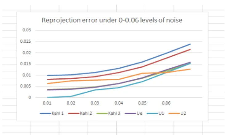
(4) Vol.2016-CVIM-201 No.1 2016/3/3. IPSJ SIG Technical Report. Pi ∈ R3×4 : i-th camera matrix. With camera matrix P, we can compute the necessary parameters Ui , Vi (i=1,2,3) by our completed program. And assume that the measured image point in each view is at the origin (which is no restriction since it can be accomplished by changing coordinate systems). In the report [8], with this example, the reprojection error has been got by using 3 formulations such as Polynomial, Schur, Bundle. They are all famous methods for solving multiview triangulation problems proposed in recent years. On the other hand, through our proposed method by using this example, we can get three upper bounds and a lower bound introduced in this report. And the results we have got is shown in Table 3 for comparing with other 3 formulation clearly: Formulation reprojection error variables Polynomial 0.157291 1286 Schur 0.157282 86 UE 0.157247 12 U3 0.156871 9 U2 0.156325 9 Bundle 0.155998 3 L 0.152554 9 Table 3 Data from the triangulation example by our proposed method. In summary, as we see in this example, in the group which includes the upper bounds, the reprojection error which is computed by using Condition 6 is the smallest. As a conclusion, the method we proposed as Condition 6 may be better than other methods. However, this is just a simplest example, our method should be further evaluated through more numerical examples. 4.2 Numerical evaluation under Kahl’s setting Before evaluating our proposed methods under Kahl’s setting, we should explain the synthetic data in similar to the one supposed in [8] by Kahl. All simulated data was generated in the following manner. Uniformly random 3D points with coordinates within [-1,1] units were projected to cameras with focal lengths of 1 pixel. The position of cameras were randomly, bout the must be at distances of 5 units from the origin in average. The cameras’ viewing directions were also random, though biased towards the origin. In addition, the image coordinates were corrupted by zeromean Gaussian noise with varying levels of standard deviation.[8] This evaluation is main for 3-views triangulation problems, so that in each experiment, 3 camera matrix were chosen. And with the purpose of getting more ideal results, in this report, we will do 500 times with each level of noise and calculating the mean value which is seen as the final result, the function is both suitable for reprojection error and running time. 4.2.1 Comparison in L2 error Regarding bisection method, minimization problems are solved, then verify whether the optimum of minimization problem satisfies Y = XX T or not. We assume that Y = XX T is satisfied when the maximum singular value of Y − XX T is lower than 1.0x10−10 . Running our program for computing reprojection error and. c 2016 Information Processing Society of Japan ⃝. running time, the results we get can be a good element for comparing with our methods just as Schur in 3 orders which is proposed in past time and worked well in the example in section 4.1. And the result of comparing among three types of orders for convex relaxation such as first convex relaxation, second convex relaxation and third convex relaxation, and our proposed methods besides Condition 2, Condition 6, Condition 7, has been given as follows: Table 4: Average upper bound of L2 error . The method corresponding relationship with the name showing in following table is like this: (1) The existing method using first convex relaxation called Kahl 1; (2) The existing method using second convex relaxation called Kahl 2; (3) The existing method using third convex relaxation called Kahl 3; (4) Method for computing an upper bound proposed by Endo in [7] called U E ; (5) Our proposed method 2 as Condition 5 called U1 ; (6) Our proposed method 3 as Condition 6 called U2 ; Noise Kahl 1 Kahl 2 Kahl 3 UE U1 U2 0 0.00987 0.00809 0.00359 0.00344 3.72E-12 0.00636 0.01 0.0102 0.00842 0.00388 0.00379 0.00057 0.00738 0.02 0.0112 0.00939 0.00481 0.0046 0.00334 0.00784 0.03 0.0131 0.0112 0.00631 0.0063 0.0044 0.00806 0.04 0.0159 0.0138 0.00865 0.00886 0.00705 0.01089 0.05 0.0199 0.0176 0.0119 0.0123 0.01116 0.01123 0.06 0.0239 0.02144 0.01533 0.01576 0.01521 0.01271 Table 4 Reprojection error by using 6 methods for computing upper bound in 0-0.06 levels of noise. Fig. 1. Reprojection error by using 6 methods for computing upper bound in 0-0.06 levels of noise. Considering the results we have obtained through numerical evaluation: Comparing with the method proposed by Kahl in 3 order, our proposed method as Condition 6 for computing the upper bound may works out the smallest upper bound under Kahl’s setting. And in high level of noise, our proposed method 3 may be better than ours. However, as one and the only lower bound, there is no another lower bound to compare with. Further, we have used the upper bound which are worked well in the experiments done in our report for comparison. And the lower bound of reprojection error which is computed by using our proposed method as Condition 5 is shown as follows: Table 5: Relation among upper and lower bounds. The method corresponding relationship with the name showing in following table is the same as Table 4. And the only one which has not 4.

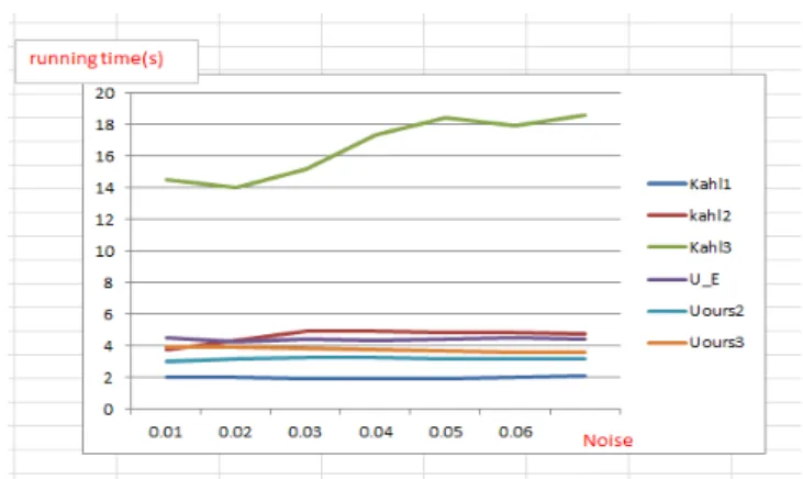
(5) Vol.2016-CVIM-201 No.1 2016/3/3. IPSJ SIG Technical Report. mentioned in Table 4 is lower bound named method 1. Noise L U1 0 7.28E-11 3.72e-12 0.01 0.00029 0.000596 0.02 0.00090 0.003343 0.03 0.002531 0.00316 0.04 0.00565 0.007045 0.05 0.00595 0.01116 0.06 0.00790 0.01521 Table 5 Reprojection error of computing lower noise. U2 0.00636 0.00738 0.00784 0.0081 0.01089 0.0112 0.03715 bound in 0-0.06 levels of. Fig. 3. Running time of each time in 0-0.06 levels of noise. Noise 0 0.01 0.02 0.03 Running time 2.887267 2.906455 2.918779 2.922616 Noise 0.04 0.05 0.06 Running time 2.925816 2.936469 2.936727 Table 7 Running time of computing lower bound in 0-0.06 levels of noise. Fig. 2. Lower bound in 0-0.06 levels of noise comparing with upper bound. During computing the upper bound by using proposed method 2, an amazing event had been appeared. That is, bad result which is too large even over 100 had been appeared randomly. It is so inconceivability that one more experiment had been done by using the same reprojection matrix. Through many times of experiments, we obtained the result which is similar to the mean. However, we do not know the reason, we guess is may be cause by property of computer. As a solution, we repeated each experiment in each level of noise three times, and choose rather stable results which are the same in the same condition as the final result. 4.2.2 Comparison in running time On the other hand, running time is also an important element for evaluating methods and algorithm. And we have obtained the running time of each formulations just as follows: Noise 0 0.01 0.02 0.03 0.04 0.05 0.06 Table 6. Schur1 Schur2 1.97862 3.75806 2.04065 4.31047 1.93444 4.90249 1.91903 4.899 1.95725 4.85883 2.04979 4.83403 2.05859 4.7921 Running time by using 0-0.06 levels of noise. Schur3 Bisection U1 U2 14.5084 4.49283 3.03734 3.94215 13.9983 4.27755 3.156 3.90315 15.1640 4.44759 3.24482 3.88599 17.3896 4.34463 3.24950 3.77990 18.470 4.40703 3.172 3.65978 17.9507 4.48659 3.20582 3.63482 18.5777 4.41527 3.187 3.61142 6 methods for computing upper bound in. Based on the running time, we know that our proposed methods is faster than the method proposed by Kahl in order 3 which is works well in computing upper bound. On the other hand, the ones proposed by us is much slower than Kahl’s method in order 1.. 5. Conclusion In this report, we have proposed several methods for computing upper and lower bounds of L2 error of multiview triangulation problems. In detail, two methods for computing upper bounds such as the Condition 6 and Condition 7 introduced in the report, and one method for calculating lower bound which is introduced as Condition 5. Our proposed methods are represented by convex linear matrix inequalities (LMI), and they are easily implemented by MATLAB using tools for handling LMI constraints such as SeDuMi and YALMIP. In this report, we not only proposed our methods for solving multiview triangulation problems, but also evaluating our methods by comparing with Kahl’s and Endo’s methods which are proposed in recently years. And we have chosen a simple virtual digital example which is given in chapter 5 of Kahl’s paper and more numerical examples by using synthetic data which are randomly. With the results, we have realized that our proposed method as Condition 6 for computing upper bound is relative usefulness than other methods in low level of noise. And our method as Condition 7 works well in high level of nose. On the other hand, the method as Condition 9 is the only one for computing lower bound, even though the difference between it and smallest bound is little, it need to validate effectiveness. Further research in finding out the much more lower bound which we would like to deal with in the future. References [1] [2] [3] [4] [5]. c 2016 Information Processing Society of Japan ⃝. R. Hartley and A. Zisserman: Multiple View Geometry in Computer Vision, Cambridge University Press, 2004. R. Hartley and F. Kahl: Optimal algorithm in multiview geometry: In Asian Conf. Computer Vision, pp. 13–34, 2007. W. Triggs, P. F. McLauchlan, R. Hartley, and A. Fitzgibbon: Bundle adjustment for structure from motion, In Vision Algorithms: Theory and Practice, pp. 298–372, 2000. H. Stewenius, F. Schaffalitzky, and D. Nister: How hard is 3-view triangulation really? In International Conf. on Computer Vision, pp. 686–693, 2005. R. Hartley, F. Kahl, C. Olsson, and Y. Seo: Verifying global minima for L2 minimization problems in multiple view Geometry, International Journal of Computer Vision, Vol. 101, No. 2, pp. 288–304,. 5.

(6) IPSJ SIG Technical Report. [6] [7]. [8] [9]. Vol.2016-CVIM-201 No.1 2016/3/3. 2013. D. Henrion, and J. B. Lasserre: Convergent relaxations of polynomial matrix inequalities and static output feedback, IEEE Transactions on Automatic Control, Vol. 51, No. 2, pp. 192–202, 2006. T. Endo, Y. Ito, and N. Babaguchi: LMI-based method for 2-norm optimization in triangulation problems, (in Japanese), IPSJ SIG Technical Report on Computer Vision and Image Media, Vol.2013-CVIM187, No. 8, pp. 1–8, 2013. F. Kahl and D. Henrion: Globally optimal estimates for geometric reconstruction problem, International journal of Computer Vision, Vol. 74, No. 1, pp. 3–15, 2007. J. F. Strurm: Using SeDuMi 1.02, a MATLAB Toolbox for Optimization over Symmetric cones, Optimization Methods and Software, Vol. 11, No. 1-4, pp. 625–653, 1999.. c 2016 Information Processing Society of Japan ⃝. 6.

(7)