Workload Classification and Performance Analysis using Job Metrics in the K computer

全文

(1)Vol.2017-HPC-162 No.13 2017/12/19. IPSJ SIG Technical Report. Workload Classification and Performance Analysis using Job Metrics in the K computer Masaaki Terai1,a). Riku Kashiwaki2,b). Fumiyoshi Shoji1,c). Abstract: In the K computer, the job manager and peripheral tools collect various metrics and store them into databases. A part of the metrics is directly provided to users by the job manager. Also, some part of the metrics is summarized and reported by administrators. However, most of the data are not fully exploited for analysis to help inform our operations because the amount of data stored in databases is growing every moment and becoming huge size that is difficult to handle them. In this study, to get the picture of workloads behavior regarding arithmetic, memory access, and I/O intensive, we attempt to classify the workloads based on modern statistics. At first, before classification of the workloads, we analyze metrics behavior as a preliminary study by PCA and select features to be used in classification. After that, we partition the workloads into several groups by k-means and DBSCAN clustering methods with 10,000 sampling workload records extracted from nearly one million records in the database. Based on the results, we obtain a few groups that require a diagnosis of the performance improvement. One of the group consists of 2,142 and 845 workloads classified by k-means and DBSCAN, respectively. Furthermore, we evaluate the validity of the classification results by normalized mutual information score. In this evaluation, based on our practice, we assume that the discipline fields are related to application performance and use the information of disciplinary field, group-id, and user-id as a label. The result shows that between these labels and application performance are less relevant. Keywords: workload classification, unsupervised classification, K-computer, performance analysis, k-means, DBSCAN. 1. Introduction As part of the operations of our supercomputing center, our division currently addresses a usage survey of our facility that includes understanding workload characteristics with statistical analysis and finding issues from a massive number of workloads in the system[1], [2]. We expect that the study helps not only demand analysis of the procurement process but also screening of applications underutilizing computing resources, detecting an anomaly workload, and choosing benchmark programs, and so on. The organized information based on usage statistics is expected to provide insights on how to improve our services. In the K computer (hereinafter referred to as K/K-computer) [3], [4], the job manager collects various usage metrics (e.g., job name, number of nodes, elapsed time, maximum memory usage, I/O usage, number of staging files, staging file size, and raw data of hardware counters) for each job, which constitutes a workload. In operation, these metrics are automatically collected and stored in databases. A part of the metrics is directly provided to users by the job manager after completion of each job. Also, some part of the metrics is summarized and reported by administrators us1. 2. a) b) c). RIKEN Advanced Institute for Computational Science, Kobe, Hyogo, 650–0047, Japan Graduate School of Simulation Studies, Univeristy of Hyogo, Kobe, Hyogo, 650–0047, Japan [email protected] [email protected] [email protected]. ⓒ 2017 Information Processing Society of Japan. ing kind of a monthly report. However, most of the data are not fully exploited for analysis to help inform our operations because the amount of data stored in databases is growing every moment and becoming huge size that is difficult to handle them. At this moment, we struggle with this kind of engineering to exploit significant information from the massive data. Recently, in order to obtain more meaningful information about workload performance from huge system logs, machine learning or some statistical techniques are attracted [5], [6], [7], [8], [9], [10], [11]. One of the statistical techniques, clustering is a fundamental multivariate analysis technique to divide the entire data set into small groups and easily understand behavior group by group without training data set. This is an appropriate method for systematically classifying unlabeled workloads in this case. Before classifying the real workloads executed on K, as preprocessing to sort out the metrics, we attempt to study metric behavior by principal component analysis and select features from the metrics. Also, we make a small data set extracted from the original data by random sampling to reduce memory usage in classification processes. After that, we attempt to classify the data set by two kinds of clustering methods: k−means and DBSCAN. Based on the classification results, we analyze the workloads characteristics of each group regarding performance (e.g., FLOPS, memory throughput, and I/O intensive) and perform screening of underutilizing application that has room for performance improvement. Finally, we evaluate the validity of the classification results by normalized mutual information score. 1.

(2) Vol.2017-HPC-162 No.13 2017/12/19. IPSJ SIG Technical Report. All the analyses were mainly performed by SciPy, scikit-learn, and pandas in Python. In the rest of the paper, we describe an overview of the job metrics and workloads of the K computer in Chapter 2. We then describe the metrics behavior and preprocessing as a preliminary in Chapter 3. In Chapter 4, we report the experiment results by k-means and DBSCAN. In Chapter 5, we evaluate the validity of the classification. Two-column size figures are added in the Appendix.. 2. K-computer K-computer is the first 10-petaflops supercomputer developed by RIKEN and Fujitsu under the Japanese national project. The system has 82,944 compute nodes connected by Tofu high-speed interconnects. Each compute node has a SPARC-V9 based customized chip called SPARC64VIIIfx [12] and is equipped with 16 GB memory for each compute node. Furthermore, a 30 PB global storage and an 11 PB local storage are installed and are transparently accessed by compute nodes through I/O nodes. 2.1 Hardware Counters The SPARC64VIIIfx chip has built-in hardware counters to store the counts of events (e.g., the number of cycles, floating instructions, load/store instructions, cache misses, and bus transactions in terms of memory and I/O read/write accesses). To precisely measure application performance with a profiler, 56-type counters are to be unlocked to users and extremely low overhead profiling is to be achieved compared with ordinary samplingbased profiling. However, the number of counters in a single execution of a user program is limited by the mechanism and the user program cannot simultaneously use more than eight hardware counters. Besides, users cannot change a set of hardware counters during the execution. Therefore, in this study, we use a single set of counters throughout the duration to consistently compare the same metrics between all targeted workloads. 2.2 Job Record Extraction From the Database For system efficiency, K-computer employs a job manager, peripheral system software, and tools, which are similar to most supercomputers. The job manager controls submitted jobs as a basic unit of workload and exclusively executes them on compute nodes. At the same time, the job manager records the time stamp, state, and various metrics of the workload in a database.. (a). Fig. 1. (b). The number of workloads/jobs and node-time based on actual records in each half-year period from 2015 to 2017.. Also, for usability enhancement, the job manager provides various job submitting methods (e.g., batch and interactive job types, ⓒ 2017 Information Processing Society of Japan. normal, bulk, and step job models) to users. Fig. 1 shows the number of jobs and node-time in each half-year period from Apr. 2015 to Sep. 2017. As shown in Fig. 1 (a), at least, each period has 130 thousand valid jobs except for invalid jobs including canceled jobs by users, statistically spoiled jobs with missing values, abnormally terminated jobs and so on. These invalid jobs account for up to 34% of the number of all jobs. On the other hand, these jobs spent up to 7% of the node time of all job. This number is sufficiently small, therefore, the invalid jobs are ignorable. Furthermore, we extracted records of the batch job type with the normal model from the database and use the extracted data set in classification because this type of record is obviously dominant and accounts for more than 90% of all the records on K, as shown in Fig. 1 (b). Also, other types of records in the bulk, step, and master-worker job models have a slightly cumbersome structure because of the parent-child relationship. In addition, the interactive job spends much time for an idle state because of waiting for the key-in command by a user. (This “interactive” type job provides a command prompt on a compute node. A user can interactively enter commands to start the user’s program.) Classifying workloads based on their performance records may make them noise information. Finally, we use the valid records from the database, except for the above conditions.. 3. Preliminary 3.1 Job Metrics and Preprocessing The job manager and peripheral tools collect more than 120 metrics for each job and store them into databases. Through the database, we can refer to eight hardware counters (While “max cycle counts” is a cycle counts in a thread, “cycle counts” is whole of cycle counts in all threads. One metric constitutes the other metric. Thus we do not include the eight counters.): “cpu mem read ratio”, “cpu mem write count ratio”, “floating inst ratio”, “fma inst ratio”, “simd floating inst ratio”, “simd fma inst ratio”, “sleep cycle ratio”, and “cycle count.” Most of the metrics including the hardware counters are integertype variables. However, part of the metrics (e.g., cycle counts and sleep cycle) easily become a large number represented by a 128-bit integer. Also, their counts depend on the duration of a workload. To equally compare metrics between workloads given three performance types: arithmetic, memory access, and I/O intensive workload. In the viewpoint of the single-node performance, they do not depend on the number of nodes. Therefore, we normalized the eight hardware counters by using “cycle counts.” Also, before the classification of the workloads, to easily handle them, we eliminated the categorical metrics (e.g., user-id, group-id) and time stamp from the original data set and then obtained 30 metrics as shown in Table 1. One of the metrics, “cycle counts” is used for the normalization of the hardware counters, but it is omitted from the table. In addition, we use the well-recognized fact that a classification process sufficiently works with lower accuracy than the accuracy of the actual measurement. Therefore, we treated all the metrics as a 32-bit floating-point number. In this study, to classify the workloads, we use only the metrics 2.

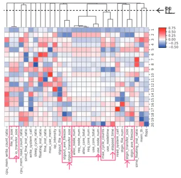
(3) Vol.2017-HPC-162 No.13 2017/12/19. IPSJ SIG Technical Report. Table 1 Job Metrics metric name alloc core total alloc node num cpu mem read count ratio cpu mem write count ratio elapsed time file io size floating inst ratio flops fma inst ratio io transfer size max cycle counts max use mem mem th op intensity read system call req core num req node num simd floating inst ratio simd fma inst ratio sleep cycle ratio stgin ave filesize stgin file num stgin transfer size stgout ave filesize stgout file num stgout transfer size use core total use node num use nodetime write system call. description num of cores actually allocated to compute nodes num of nodes actually allocated to compute nodes cpu memory read counts per cycle counts cpu memory write counts per cycle counts elapsed time in a job file I/O size floating inst. counts per cycle counts num of floating-point op. per elapsed time (FLOPS) FMA inst. counts per cycle counts I/O transfer size max cycle counts in all threads max memory usage in a compute node memory throughput arithmetic intensity (=flops/mem th) num of read system call num of cores required by a job script num of nodes required by a job script SIMD-floating inst. counts per cycle counts SIMD-FMA inst. counts per cycle counts sleep cycle counts per cycle counts average file size in stging-in num of files in stging-in total file size in stging-in average file size in stging-out num of files in stging-out total file size in stging-out num of cores actually used for a workload num of nodes actually used for a workload product of use node num and elapsed time num of write system call. metrics is not much different from the rate with all metrics. On the other hand, the rate with six metrics exceeded 80% of all the metrics contribution. In other words, only six metrics can reserve most of the original information in multidimensional space. Generally, 30 metrics is not a large number as compared to other data mining projects based on natural language processing with more than ten-thousand features. However, we determined to use 20 metrics based on the result because the reduction of the features is directly linked to memory usage and computation time.. as shown in the table. 3.2 Log-transformation The metrics have substantially left-skewed distribution. To be spread between records more uniformly, we apply the logarithmic transformation defined by eqn. (1), where v = u + 1(u ≥ 0) and u is a actual measurement value of a metric. w = ln (v). (1). Fig. 2 Cumulative PCA contribution rate. The horizontal axis is the number of PCA components. The vertical axis is the contribution rate.. Fig. 3 shows the loading factors between the metrics and PCA components with heatmap. This result reveals the correlations of the metrics for each PCA component. Obviously, the metrics related to the number of nodes or cores are strongly same behavior. Also, “file io size” and “io transfer size” is very similar.. After then, we apply standardization to the log-transformed value as eqn. (2), where wmean is the mean value and w sd is the standard deviation for w. (w − wmean ) w std = (2) w sd. 20. Finally, after the rescaling process, we obtained preprocessed data sets. This transformation has pros and cons. Most of the correlations between the metrics tend to be positive because the magnitude of the metric value except for normalized value (e.g., ratio) depends on duration (e.g., elapsed time). While this transformation improves an appearance of the shape of distribution on subspace, it may needlessly emphasize the correlation between the metrics. 3.3 Feature Selection with PCA Some metrics (e.g., req node num, alloc node num, and use node num) are experimentally expected to be similar values. Also, part of the metrics is calculated from several other metrics. For instance, “flops” is derived from a few hardware counters (e.g., floating-point instruction counts, SIMD/FMA/SIMDFMA floating-point instruction counts.) Therefore, FLOPS and the hardware counters to be used for the arithmetic are correlated each other. To determine the number of metrics to be used for classification, we evaluate the contribution rate by principal component analysis (PCA) as feature selection. As shown in Fig. 2, the cumulative contribution rate with 25 ⓒ 2017 Information Processing Society of Japan. Fig. 3. PCA loading factors. The rows mean the metrics. The columns mean the PCA components. The heat map with dendrogram uses the standardized values for each metrics. The dendrogram was calculated by hierarchical clustering with the Euclidean distance and the Ward variance minimization algorithm as a linkage method. Each arrow means feature selection based on the result of the dendrogram.. To find out metrics with similar behavior, we calculated hierarchical clustering and show the dendrogram on the top of the 3.

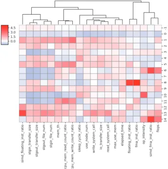
(4) IPSJ SIG Technical Report. Vol.2017-HPC-162 No.13 2017/12/19. figure. Based on the result, we obtained an optimal set of features to classify. 3.4 Random Sampling In this study, we used the data set collected from five half-year periods, Spr. 1, 2015 to Sep. 30, 2017. The number of targeted workloads is 911,544. However, a few clustering methods including DBSCAN require much computation time and memory consumption. As an early study, we do not need classification using all workloads. To reduce the calculation time and memory usage, we use random sampling and make new data set consists of 10,000 workloads from the original record. We confirmed that the new data set is statistically same as the original using two-sided Kolmogorov–Smirnov test with 0.05 as a significance level.. 4. Experiments In this chapter, we classify the actual workloads by k-means and DBSCAN[13] (Density-based spatial clustering of applications with noise.) Both are the common and robust clustering methods to divide data into several small groups without training data set. 4.1 k-means k-means is a partitioning clustering method and requires two kinds of parameters: vector of initial centroids and number of clusters. Determining the initial centroids are an essential factor to obtain a preferable classification. The scikit-learn provides k-means++ implementation that automatically performs preprocessing to choose optimal initial centroids. During several trials of the classification in this study, we confirmed that these preprocessed centroids are very stable even though the algorithm uses random numbers. Therefore, hereafter, we can focus on determining the number of clusters.. Fig. 4. Residual sum of squares in the k-means classification.. We classified with the number of clusters k from 2 to 50. Fig. 4 shows the residual sum of squares. Based on the result, we can find out some steep points with the elbow method and chose k=7, 16, and 33. Fig. A·1 shows the result of the clustering by k-means with k=7, 16, and 33, respectively. As well-known characteristics of k-means, it tends to make similar size groups relative to other clustering methods. These results represent the characteristics. ⓒ 2017 Information Processing Society of Japan. Fig. 5 The metrics vs. clusters in k-means classification with #cluster=7. The rows of the heat map are cluster number. The columns are the metrics. A heat map with dendrogram uses the standardized values for each metrics. The white color represents the mean value in a column. The red and blue color describe the values higher and lower than the mean value, respectively.. To obtain standardized values based on the metrics and clusters, at first, we calculated an average of the metric values for all data of each column. In addition, we calculated an average of the metric for each column in a cluster. And then, using the average values of all data set and a classified data set for each column, we performed standardization for each column, cluster by cluster. Finally, we obtained the heat map with the number of clusters k = 7 as shown in Fig. 5. Hereafter, with the figure, we see the characteristics based on the metrics, cluster by cluster. At first, regarding the staging metrics, cluster-0 has values lower than the mean of all clusters. On the other hand, I/O metrics (“io transfer size” and “read system call”) slightly have high value, while arithmetic and memory access metrics (“flops” and “mem th”) have low values. Interpreting the group is difficult. At this moment, we estimate the cluster is a kind of weak I/O intensive workloads. Cluster-1 has the highest values in arithmetic metrics (“floating inst ratio” and “fma inst ratio.”) In addition to those, other arithmetic metrics (“flops” and “op intensity”) have higher values than the mean. We think that these classified workloads are a kind of arithmetic intensive. But the number of workloads is the smallest. Therefore, we can determine that the workloads are low-priority to check than others. In cluster-2, all the metrics have values lower than the mean. Also, these workloads used a small number of nodes in less time. In other words, the workloads are ignorable. Cluster-3 has high values on the whole and seems the most resource consuming cluster. Also, the cluster has a characteristic of I/O intensive with a large number of nodes. Also, the cluster has the highest value in the memory throughput metric (“mem th”) and high values in staging metrics. We are impressed that the cluster exploits more compute resources than others. 4.

(5) Vol.2017-HPC-162 No.13 2017/12/19. IPSJ SIG Technical Report. Cluster-4 has the highest arithmetic and high memory access metrics values (“flops”, “mem th”, and “op intensity.”) On the other hand, I/O and staging metrics have lower values than the mean. Also, the workloads have higher values regarding a magnitude of workload (“use node num” and “elapased time”) than the mean. The workloads have the prominent characteristics of arithmetic intensive. Cluster-5 is similar to cluster-2 except for staging metric values. Also, the memory usage metric (“max use mem”) is nearly equal to the mean. We think the workloads are lowpriority to check in more detail because the magnitude metrics (“elapsed time” and “use node num”) are smaller than the mean. In cluster-6, while the workloads have lower arithmetic and memory access metrics (“flops” and “mem th,”) they have higher values in the magnitude metrics (“use node num” and “elapsed time.”) Also, the number of the workloads is the largest through all clusters according Fig. A·1. Concerning the application performance improvement, the workloads are the most important candidate to check in more detail. Finally, regarding workloads performance, we think that the characteristics of cluster-6 need to be examined in more detail because these workloads of the cluster used much node-time larger than the mean and have lower values in terms of arithmetic and memory access. In addition, they are approximately 2,000 in the sampling data set. The sampling data set consists of 10 thousand workloads records extracted from nearly million workloads, the fact means that there are underutilizing 200-thousand workloads in K. If this naive conclusion is true, the number of workloads in the cluster cannot be ignored. 4.2 DBSCAN DBSCAN is a density-based clustering method and requires two parameters instead of the number of clusters k in k-means. One is the maximum radius to search the neighborhood (hereafter referred to as eps), similar to cut-off distance in molecular dynamics simulation. The other is a criterion (hereafter referred to as minPts) to connect a targeted point (workload record) to a cluster or drop the point as noise. If the number of points of workloads inside the radius exceeds the minPts, the point is connected to a cluster. This is one of the characteristics of DBSCAN. If the point eventually does not belong to any clusters, this method treats the point as noise information. Therefore, determining the eps and minPts are an essential factor to obtain an appropriate classification. Fig. 6 shows the number of clusters along with the parameters: eps and minPts. While small eps generates a large number of clusters (This parameter generates more than 80 clusters in minPts=10 and eps=1.0.), Using large eps, DBSCAN does not correctly work to classify the workloads because each point easily connects to one large cluster. This cluster is not different from noise. Based on the result, we determined the appropriate parameter range: eps=1.0 to 2.0 and minPts=50 to 80. Fig. A·2 shows the workloads classified by DBSCAN. Each 3 × 3 figure block along with the parameters (eps and minPts) consists of a set of two figures: clustered and noise. We can see the characteristics that too large eps incurs a single large clusⓒ 2017 Information Processing Society of Japan. Fig. 6. The number of clusters in the parameter-sweep experiments of DBSCAN with eps=1.0 to 2.5 and minPts=10 to 100.. ter as well as noise. Also, too large minPts prevent the growth of clusters. Also, DBSCAN does not depend on assuming the hypersphere for the shape of a cluster. We can see the shape of clusters with vertically/horizontally long, that is different from the shape by k-means. Fig. A·3 shows the number of workloads for each cluster. Negative cluster number means noise. Based on the result, we think that the data set includes so many noisy information to prevent the growth of clusters. In other words, most of the workloads are sparsely distributed over the subspace. The density is very low on the whole.. Fig. 7. Heat map of the metrics vs. clusters in classificaiton by DBSCAN with eps=1.5 and minPts=50.. As well as the evaluation with k-means, we obtained the metric values cluster by cluster, as shown in Fig. 7. DBSCAN divides the data set into 14 groups and noise. We omitted clusters with a small number of workloads and eventually chose cluster#=0, 1, 3, 4, and 6. Other clusters are ignorable in terms of the number of workloads. Cluster-1 is the largest cluster except for noise and reaches 5.

(6) Vol.2017-HPC-162 No.13 2017/12/19. IPSJ SIG Technical Report. 2,800 workloads in the sampling data set. However, based on the result, all the metric values are lower than the mean. In other words, most of the workloads are lower performance than the mean. We think that the workloads are ignorable. In cluster-3, the staging metrics have lower values than the mean. While the magnitude metric (“use node num”) is slightly large, another magnitude metric (“elapsed time”) is smaller than the mean. The memory throughput metric (“mem th”) is nearly equal to the mean. We think that the workloads are the most important candidate to be checked in more detail. The number of workloads in the cluster is 845. Cluster-4 has lower values than the mean in the arithmetic and memory access metrics (“flops” and “mem th.”) On the other hand, the I/O metric (“io transfer size”) is larger than the mean. Also, the memory usage metric (“max use mem”) has high value. We think that the workloads are a kind of I/O intensive. Cluster-6 has the highest values in the arithmetic and memory access metric (“flops” and high “mem th.”) The workloads are typical computation intensive. Through the experiments, we confirmed that the scikit-learn’s implementation works well. However, it consumes a lot of memory usage than other implementation (e.g., pyclustering). This is an issue depending on the implementation of DBSCAN. If we attempt to classify a million workloads, a kind of high-performance technique will be required in future of our study.. 5. Evaluation and Discussion In the previous chapter, we confirmed that both clustering methods divided into small groups and found that a few clusters become candidates for diagnosis of the performance improvement. On the other hand, we need to confirm that the experiments correctly perform to partition the workloads into small groups, while we do not have any kinds of criteria (e.g., training data set) to know the validity of the classification. Therefore, we used an assumption based on our heuristics in this evaluation. In our operations, we often assume the relationship or correlation between application performance and disciplinary field (e.g., biological science, material science, environmental science, engineering and fundamental physics) on statistical average because each field frequently uses a similar model, scheme, and library. Based on our practice, we exploited the disciplinary field information as a workload’s label. In addition to that, we used groupid and user-id as a label as well in order to confirm the validity under the assumption. These labels are used for the evaluation process, not for the classification. The number of “fields” is six. Also. The number of group-ids and user-ids are 282 and 882 in the data set, respectively. For group-id and user-id, we confirmed that there are no missing values in the data set. On the other hand, part of workloads does not have the “field” label because the “field” label is assigned by manual based on the usage reports. Thus, we assigned “misc” label to those workloads. Furthermore, to quantitatively compare clustered workloads with assigned labels, we used normalized mutual information (NMI) [14] as defined by eqn.6, where N is the number of workloads, K is the number of clusters, and J is the number of labels. ⓒ 2017 Information Processing Society of Japan. Eqn.3 and Eqn.4 express entropy of the set of clusters and labels, where ωk is a set of workloads in k-th cluster, c j is a set of workloads labeled as j. Eqn.5 expresses mutual information, where ωk ∩ c j is a set of workloads with j-label in k-th cluster. NMI is a common criterion based on entropy expression in information retrieval. The range of value is from 0.0 to 1.0. If all workloads are completely divided into different clusters along with labels under the condition that the number of clusters equals the number of labels, NMI score is 1.0. In the condition of our study, the number of clusters is not equal to the number of labels. However, if wellseparated clusters along with labels, the entropy decreases; NMI increases. K ∑ |ωk | |ωk | H(Ω) = − log (3) N N k H(C) = −. J ∑ |c j | j. I(Ω; C) =. N. log. |c j | N. (4). K ∑ J ∑ |ωk ∩ c j | k. N MI(Ω; C) =. j. N. log. N|ωk ∩ c j | |ωk ||c j |. I(Ω; C) [H(Ω) + H(C)]/2. (5). (6). Table 2, 3, and 4 show NMI scores under the conditions that the number of clusters is 9, 14, and 45 based on the result with DBSCAN as mentioned in the previous chapter. NMI is less than 0.5 in most of the cases. Also, while NMI scores in DBSCAN are smaller than k-means for the “field” label, both values in k-means and DBSCAN are very low. We think that the “field” label does not represent the behavior of major applications due to a lot of noisy workloads, or this criterion is not appropriate in terms of diagnosis of the application performance. On the other hand, for the group-id and user-id, the NMI scores improve. However, we think that the number of labels regarding group-id and user-id is too large to classify. In other words, too many labels cause fitting into too many small clusters. Table 2 NMI (#cluster=9) label field group-id user-id. k-means 0.16 0.31 0.36. DBSCAN 0.24 0.27 0.28. Table 3 NMI (#cluster=14) label field group-id user-id. k-means 0.18 0.35 0.42. DBSCAN 0.26 0.32 0.34. Table 4 NMI (#cluster=45) label field group-id user-id. k-means 0.23 0.48 0.55. DBSCAN 0.31 0.43 0.46. Based on the results, finding some criteria to evaluate the validity of the classification result is one of importance in our research. We need to solve the problem in future if the information is exploited for some tasks in our operations. 6.

(7) Vol.2017-HPC-162 No.13 2017/12/19. IPSJ SIG Technical Report. 6. Summary In this paper, we introduced and discussed our current research regarding data mining with the metrics of the massive workloads on K. The job manager and peripheral tools collect various metrics and store them into databases. A part of the metrics is directly provided to users by the job manager. Also, some part of the metrics is summarized and reported by administrators using kind of an annual report. However, most of the data are not fully exploited for analysis to help inform our operations because the amount of data stored in databases is growing every moment and becoming huge size that is difficult to handle them. As an early study, to get the picture of workloads behavior based on modern statistics, we classified the workloads and analyzed their performance characteristics group by group. Based on the classification, with 10,000 sampling records extracted from the nearly million records in the original database, we found the candidates to be checked in more detail. Each cluster consists of 2,142 and 845 workloads classified by k-means and DBSCAN, respectively. Furthermore, we evaluated the validity of the classification results by normalized mutual information score. In this evaluation, based on our practice, we assumed that the disciplinary fields for users group are related to application performance. Under the assumption, we used the field, group-id, and user-id as a label. The result showed that between these labels and application performance is less relevant. We need to solve the problem in future if the information is exploited for some tasks in our operations.. [7]. [8]. [9] [10]. [11]. [12] [13]. [14]. Commodity Clusters: An Empirical Study of a Tapered Fat-tree, Proc. of the Inter. Conf. for High Performance Comp., Networking, Storage and Analysis, SC ’16, IEEE Press, pp. 78:1–78:12 (2016). Liu, Y. et al.: Server-Side Log Data Analytics for I/O Workload Characterization and Coordination on Large Shared Storage Systems, SC16: Inter. Conf. for High Performance Comp., Networking, Storage and Analysis, pp. 819–829 (online), DOI: 10.1109/SC.2016.69 (2016). Ahn, D. H. et al.: Scalable Analysis Techniques for Microprocessor Performance Counter Metrics, Proc. of the 2002 ACM/IEEE Conf. on Supercomputing, SC ’02, IEEE Computer Society Press, pp. 1–16 (2002). Xing, F. et al.: HPC Benchmark Assessment with Statistical Analysis, Procedia Computer Science, Vol. 29, No. Supplement C, pp. 210 – 219 (online), DOI: https://doi.org/10.1016/j.procs.2014.05.019 (2014). Xing, F. et al.: Statistical Performance Analysis for Scientific Applications, Proc. of the 2014 Annu. Conf. on Extreme Sci. and Engineering Discovery Environment, XSEDE ’14, ACM, pp. 62:1–62:8 (online), DOI: 10.1145/2616498.2616555 (2014). Tuncer, O. et al.: Diagnosing Performance Variations in HPC Applications Using Machine Learning, High Performance Comp. - 32nd Inter. Conf., ISC High Performance 2017, Frankfurt, Germany, June 18-22, 2017, Proc., pp. 355–373 (2017). Fujitsu Limited: SPARC64VIIIfx Extensions (2010). Ester, M., Kriegel, H.-P., Sander, J. and Xu, X.: A Density-based Algorithm for Discovering Clusters a Density-based Algorithm for Discovering Clusters in Large Spatial Databases with Noise, Proceedings of the Second International Conference on Knowledge Discovery and Data Mining, KDD’96, AAAI Press, pp. 226–231 (1996). Manning, C. D., Raghavan, P. and Schütze, H.: Introduction to Information Retrieval, Cambridge University Press, New York, NY, USA (2008).. Appendix A.1. k-means. Fig. A·1 is added in the appendix.. A.2 DBSCAN Fig. A·2 and Fig. A·3 are added in the appendix.. Acknowledgments This research was supported by Akiyoshi Kuroda, Katsufumi Sugeta, Keiji Yamamoto, Shun Ito, and our colleagues in RIKEN AICS and Ryuichi Sekizawa and Shunsuke Inoue of Fujitsu. We thank Kazuo Minami of RIKEN AICS, Masatomo Hashimoto and Toshiyuki Maeda of Chiba Institute of Technology, and Yutaka Hata of the University of Hyogo for providing insights and comments that greatly assisted the research. Part of the results is obtained by using the K computer at the RIKEN Advanced Institute for Computational Science. References [1] [2] [3]. [4]. [5]. [6]. Kuroda, A. et al.: Development of Job Analysis for Power-saving and Operational Improvement on the K computer (in Japanese), IPSJ SIG Technical Report, Vol. Vol.2016-HPC-156, No. No.7 (2016). Kuroda, A. et al.: Analysis of the Correlation between Application Performance and Power Consumption on the K Computer (in Japanese), IPSJ ACS, Vol. 8, No. 4, pp. 1–12 (2015). Yokokawa, M. et al.: The K computer: Japanese next-generation supercomputer development project, IEEE/ACM Inter. Sym. on Low Power Electronics and Design, pp. 371–372 (online), DOI: 10.1109/ISLPED.2011.5993668 (2011). Yamamoto, K. et al.: The K computer Operations: Experiences and Statistics, Procedia Comp. Sci., Vol. 29, No. Supplement C, pp. 576 – 585 (online), DOI: https://doi.org/10.1016/j.procs.2014.05.052 (2014). Phansalkar, A. et al.: Analysis of Redundancy and Application Balance in the SPEC CPU2006 Benchmark Suite, Proc. of the 34th Annu. Inter. Sym. on Comp. Architecture, ISCA ’07, ACM, pp. 412–423 (online), DOI: 10.1145/1250662.1250713 (2007). León, E. A. et al.: Characterizing Parallel Scientific Applications on. ⓒ 2017 Information Processing Society of Japan. 7.

(8) Vol.2017-HPC-162 No.13 2017/12/19. IPSJ SIG Technical Report. #clusters=7. (a-1). (b-1). (c-1). (b-2). (c-2). (b-3). (c-3). #clusters=16. (a-2) #clusters=33. (a-3) Fig. A·1. (a-*) The workloads classified by k-means and plotted on PCA subspace. The assigned colors (#color=20) are periodically used in a figure. (b-*) Centroids plotted on PCA subspace. (c-*) The number of workloads in each cluster.. ⓒ 2017 Information Processing Society of Japan. 8.

(9) Vol.2017-HPC-162 No.13 2017/12/19. IPSJ SIG Technical Report. eps=1.5. eps=2.0. minPts=100. minPts=50. minPts=10. eps=1.0. Fig. A·2. The workloads classified by DBSCAN and plotted on PCA subspace. Each set of parameters consists of clustered (left) and noise (right).. eps=1.0. eps=1.5. eps=2.0. 3000. Number of Workloads. Number of Workloads. 3500. 6000. 4000. 2500. 3000. 2000 1500. 4000. 2000. 1000. 2000. 1000. 500 0. 8000. 5000. Number of Workloads. MinPts=10. 6000 4000. 0. -1 4 9 14 19 24 29 34 39 44 49 54 59 64 69 74 79. cluster#. -1. 4. 9. 14. 19. 24. cluster#. 29. 34. 39. Number of Workloads. 6000. 3000. 4000. 5000 4000. 2000. 3000 2000. 3000 2000. 1000. 1000. 1000 0. −1 0 1 2 3 4 5 6 7 8 9 10 11 12 13 14 15 16 17 18 19. cluster#. 0. −1 0 1 2 3 4 5 6 7 8 9 10 11 12 13 14. cluster#. −1. 0. 1. 2. cluster#. 3. 4. 7000. 8000. 5000. 6000. Number of Workloads. 6000. Number of Workloads. 7000. Number of Workloads. MinPts=100. cluster#. 7000. Number of Workloads. 5000. 5000. 4000. 5000. 4000. 3000. 4000. 3000. 3000. 2000. 2000. 2000. 1000. 1000 0. −1 0 1 2 3 4 5 6 7 8 9 10 11 12 13 14 15 16 17. 8000 4000. 6000. Number of Workloads. MinPts=50. 7000. 0. 0. 44. −1. 0. 1. 2. 3. 4. cluster#. 5. 6. 7. 0. 1000. −1. 0. 1. 2. 3. 4. 5. cluster#. 6. 7. 8. 9. 0. −1. cluster#. 0. Fig. A·3 The number of workloads classified by DBSCAN with eps=1.0, 1.5, and 2.0 and minPts=10, 50, and 100. Cluster# = −1 is noise.. ⓒ 2017 Information Processing Society of Japan. 9.

(10)