Abstract—With more and more frequency, users communicate with each other on social media. Many users start on Twitter or Facebook to find friends who have the same hobby. Our study proposes a method to estimate the users’ interests (hobby) based on tweets on Twitter. One tweet does not, in and of itself, contain a lot of information, and some tweets are not related to the user’s hobby. Therefore, we propose a reliable hobby estimation method by extracting features from multiple, sequential tweets. The proposed method
uses Recurrent Neural Networks (RNN) which can
accommodate time-series information. We also used a Convolutional Neural Networks (CNN) which can treat contextual information. We used an averaged vector of word distributed representation as a feature. Using the proposed method based on Long Short-Term Memory Recurrent Neural Networks (LSTM-RNN), we obtained a 23.72% improvement as compared with a baseline method using a Random Forest (RF) regression as a machine learning algorithm.
Index Terms—Hobby estimation, deep neural networks,
sequential statements, social media.
I. INTRODUCTION
With more and more frequency, users communicate with each other on social media. Many users start on Twitter or Facebook to find friends who have the same hobby. Twpro [1] is a web service which can search for Twitter users who have similar attributes such as hobbies, gender, age, location, job, etc., by examining their profile information. This service is useful for finding compatible users. However, there is not always a corresponding relationship between the user's description on their profile and their tweets. Many of those accounts are only used for advertisement. In the case of an advertisement-oriented account, because the content of all their tweets is similar to each other, it is possible to automatically exclude these accounts from the target pool. On the other hand, there are cases of users who, even if their jobs, hobbies, or ages have changed, do not update their profile information. Their profiles, then, become noise for the searching algorithm. Also on Twitter, many users try to maintain a high degree of anonymity, and there are a lot of users who dissemble by publishing false attributes in their profile. Because of these factors, depending on profile information alone can be very misleading.
In this study, we propose to estimate the user’s hobby Manuscript received September 21, 2018; revised March 14, 2019. Koji Bando is with President & CEO of NTT Plala Inc., Tokyo, Japan. Kazuyuki Matsumoto is with Tokushima University, Japan (e-mail: [email protected]).
Minoru Yoshida is with Department of Information Science and Intelligent Systems, University of Tokushima, Japan.
Kenji Kita is with ATR Interpreting Telephony Research Laboratories, Kyoto, Japan.
based on their tweets on Twitter. One tweet does not, in and of itself, contain a lot of information, and some tweets are not related to the user’s hobby. Therefore, to increase the reliability, we extract features from multiple, sequential tweets. Generally, because most keywords which relate to hobbies are nouns, it is necessary to be able to accommodate proper nouns. Because proper nouns are not included in the general dictionary, the proposed method is to expand the versatility of classification by extracting word distributed representation which can better process semantic/context features.
In recent years, there have been many studies using deep-learning methods, and deep learning is effective for text classification in the present situation in which we can acquire large amounts of text-based data. The proposed method extracts an averaged, distributed representation vector from the multiple, sequential tweets. Then, we use a Recurrent Neural Network (RNN) which is a kind of deep learning which trains on the feature vector while avoiding a loss of time-series information. And, we also use a Convolutional Neural Network (CNN) which can address contextual information.
Section II describes the related research, and Section III describes the proposed method. In Section IV, we discuss evaluation experiments and the results. Finally, in Section V we present our conclusions.
II. RELATED WORKS
A. Tweet Attribute Extraction
The studies that have been done previously have analyzed users’ interests from the information on Twitter [2]-[7]. Makki et al. [8] by inducing the users’ interests from their profile information which is written by the users themselves, and some also [9], [10] consider the users’ tweets. Kapanipathi et al. [11] proposed the user interests identification method based on a hierarchical relationships present in knowledge-bases.
Because most of the profile information registered on Twitter is not updated by the user even if their hobby, age, or job changes, searching based on only extracted profile information is not very effective.
On the other hand, [12] analyzing the users’ interests by topics gleaned from their own statements can give better results. This can be done by [13], [14] estimating the users’ personalities by analyzing the users’ everyday tweets on Twitter.
On the other hand, there are a lot of studies focusing on users’ profile or attributes such as age, sex, occupation, etc. [15]-[18]. Kato et al. [15] estimated user’s attribute and habitual behavior on Twitter. Their method used not only
Twitter User’s Hobby Estimation Based on Sequential
Statements Using Deep Neural Networks
posted contents and user’s profile text but also user’s lifestyle information. To extract the opinions on commercial products and TV programs, Ikeda et al. [16] estimated users’ profiles such as age, sex, area, etc. by analyzing their opinions posted on Twitter. Rao et al. [17] investigated the feature for Support Vector Machine (SVM) based on the four types of users’ attribute classification method. Their proposed method achieved better performance than other baseline methods. However, their method is only to estimate user’s occupation not to estimate user’s interests or hobbies.
Many of these studies treat the obtained users’ tweets as one set of data, and their studies did not consider time-series information.
Fig. 1. Overview of the proposed method.
B. Social Big Data Analysis
There are a lot of existing studies of analysis of big data on Internet or social media [19]-[25]. These studies commonly focus on how to extract information from large amounts of data in formats that can be easily recognized by humans or how to analyze emotions and opinions from such large data. Vatrapu et al. [25] proposed a social set analysis. This approach consists of a generative framework for the philosophies of computational social science, etc. They used fuzzy set theory and visualized the result of analytics. Their approach could analyze users’ opinions on some enterprises for each users’ group on social media.
Sohangir et al. [26] applied several deep learning approaches such as Long Short-Term Memory, Doc2Vec and Convolutional Neural Networks to stock market opinions posted on StockTwits. They predicted sentiment (positive, negative and neutral) from the authors’ posted comments by using Convolutional Neural Networks and obtained approximately 90% accuracy.
Even though it is possible to analyze large datasets because existing computer resources are available and sophisticated calculation algorithms such as distributed computing can be developed, this approach tends to overlook information, such as minority opinions, if all the data is targeted. Therefore, it is important to narrow the range of the target for summarizing necessary information from large-size, informational datasets.
In this paper, we focus on the extraction of “hobby” which
is a fluctuating attribute by using Twitter which is an instantaneous media. Firstly, we do not use an enormous amount of data, and we validate the proposed method by conducting an evaluation experiment on the dataset which is collected under the controlled conditions.
III. PROPOSED METHOD
A. Overview of Proposed Method
The overview of the proposed method is shown in Fig. 1. In the proposed method, the user’s statements are obtained in order by posting date, and N tweets sequence is made by skipping over S tweets. In this process, it is allowed to include the same tweets in other tweet sequences.
In the obtained tweet sequences, we split the tweet into word units by morphological analysis, and converted the tweets into the a word sequence. To each word in the word sequence, the D dimension word distributed representation vectors were extracted by using the pre-trained word distributed representation model. By creating the averaged word distributed representation vector for each tweet, an 𝑁 × 𝐷 matrix was obtained for each tweet.
By training deep neural networks such as RNN, CNN using the matrix as feature X, and the estimated target Y (hobby category), the hobby category estimator which estimates the hobby category vectors from N tweet sequences were created. The multiple estimated results (hobby category vectors) were output because several tweet sequences are created for each user. We evaluate the averaged vector of the output category vectors as the final estimated result.
B. Tweet Collection
Fig. 2. Example of search result by Twpro API.
This section describes the method used to collect hobby information of the user accounts and collect the corresponding tweets. First, we obtained the account information from the Twpro website for 12 large categories. We used the Twpro API [27] for acquiring the account information. The following is an example of searching users which are matched with a facultative keyword by using Twpro API.
Training Search by Hobby
Hobby Categories
Extract sequential statements (N tweets) for each user
User ID User screen name
12345678 001xtwt 12435687 12yyyystar 12345688 chop_chop234
… …
Acquire target user list
Calculate averaged word vectors
Word Vector Matrix
Pre-trained Word Vector Model (300 dim.)
Deep Neural Networks (RNN/LSTM/GRU/CNN) 0.13, 0.22, ….. , 0.08 0.01, 0.14, ….. , 0.93 0.67, 0.51, ….. , 0.11 ・ ・ ・ Hobby Category Classifier 1) 5)
Convert into word list for each tweet by using Japanese Morphological analyzer MeCab
2)
3)
Convert into word vectors 4) I . . . . . . want . . . . . . to . . . . . . go . . . . . . . . . . . . . ! . . . . . . 0.03, 0.12, ….. , 0.24 0.21, 0.79, ….. , 0.10 6) 0.13, 0.22, ….. , 0.08 0.01, 0.14, ….. , 0.93 0.67, 0.51, ….. , 0.11 ・ ・ ・ 0 ,… ,1 ,… 0
Word vector matrix
Ex.) query=”cooking”, number of display=10 https://twpro.jp/1/search?q=cooking&num=10 The search result is shown in Fig. 2.
Next, we obtained the timeline information for each account by using the Twitter API [28]. We used Tweepy [29] as a library which uses the Twitter API on Python. We collected approximately 20 tweets for each account.
C. Word Distributed Representation: Word Embeddings
Word distributed representation is an expression which expresses words by a real-valued, fixed-dimension vector. The development of wor2vec [30], which is a learning algorithm/tool of word distributed representation from the text corpus, resulted in the rapid spread and use of word distributed representation [31]. Since a word distributed representation algorithm can train on sense-similar words that have similar vectors to each other, the algorithms are widely used for various tasks such as text classification, semantic analysis, and machine translation.
There are two main models used as the word distributed representation models: the Skip-Gram model and Continuous Bag-of-Words (CBOW) model. Both of those are trained by neural networks. Additionally, there is another method, the Global Vectors model (GloVe) [32]. GloVe is faster, has a higher accuracy than word2vec, and can work with a small corpus. It is thought that because of this reason, a higher accuracy initial value can be obtained by adding a co-occurrence matrix to the training. However, which methods are the most effective depends on the kind of task or target data.
For the experiment we describe in this paper, we used a pre-trained model [33] by fastText [34]. The number of dimensions of this vector model is 300, and it can be used with Japanese language Wikipedia articles as the training data. Because fastText can train on similar strings that have similar vectors to each other by considering character n-grams, this method can robustly differentiate a word notation or unknown expressions. The parameters of fastText are shown in Table I. The other parameters are set as the default value.
TABLEI:PARAMETERS OF FASTTEXT
Source Japanese Wikipedia articles
Size of vectors 300
Size of context window 5
Model Skip-gram
Min-count 1
The proposed method extracted the set of word distributed representation from the word sequences which were obtained by the Japanese morphological analyzer MeCab [35]. Then, the averaged vector of the vectors was generated, and this vector was compared to each tweet’s feature.
Eq. (1) is an equation for calculation of the average vector, 𝑣𝑥,which indicates the average vector of tweet 𝑥 . 𝑊𝑥
indicates the number of words in tweet 𝑥. 𝑤𝑣𝑥𝑖 indicates the
word vector of 𝑊𝑖 in tweet 𝑥.
𝑣𝑥= 𝑊1 𝑥 𝑤𝑣𝑥 𝑖 𝑊𝑥 𝑖=1 (1) D. Neural Networks
RNNs can be trained with time-series data. When inputting the sequential data, the output of the first, subsequent hidden layer is used as next input. This process can capture the data-change transition or characteristics of feature order.
In this study, we believed that the order of tweets is more meaningful than the order of words in a tweet. As Twitter is media which has high immediacy, an event tends to be expressed by multiple, sequential tweets. Therefore, it was thought that sequential tweets are highly related to each other.
On the other hand, even though the order of words has meaning, a lot of content which is posted on Twitter is very colloquial, and often only words or phrases are posted. Therefore, the co-occurrence of words is more important than the order of words.
In this study, we also used Long short-term memory (LSTM) [36] or gated recurrent unit (GRU) [37] as improved RNNs. Moreover, we used CNNs [38] which can learn the relationship between peripheral tweets but cannot learn in time-series.
Fig. 3-6 shows the network structures of RNN, LSTM, GRU, and CNN. We used softmax as an activation function of the output layer, and Adam [39] as an optimization algorithm. Softmax function is shown in Eq. (2) and Eq. (3). By using softmax function, the range of output values becomes 0 ≤ softmax(𝑜 𝑡 )
𝑖≤ 1.
And, we set the dropout rate in the output of each layer. As a loss function, we used the categorical cross entropy. Categorical cross entropy error (Loss) is calculated by Eq. (4). 𝑦(𝑡) indicates the 1-of-K representation of the training data t.
𝑦 (𝑡) indicates the model output of the data t. c indicates each
category. 𝑜𝑘(𝑡)= log𝑃(𝐶𝑘|𝑥) 𝑃(𝐶𝐾|𝑥) (2) softmax(𝑜 𝑡 ) 𝑖 = exp (𝑜𝑖 𝑡 ) exp (𝑜𝐶 𝑐 𝑡 ) (3) Loss = − 𝑦𝑡 𝑐 𝑐(𝑡)log𝑦 𝑐(𝑡) (4)
Fig. 3. Network structure of RNN.
Fig. 4. Network structure of LSTM.
We used Keras version 2.1.1 [40] in the construction of each of the networks and used TensorFlow version 1.4.0 [41] as a backend framework. The maximum iteration number was set at 10. And, we used an early stopping method which stops the training when the categorical cross entropy error
Input Layer Input: (None, N, 300) ---Output: (None, N, 300) RNN Layer-1 Input: (None, N, 300) ---Output: (None, N, 128) RNN Layer-2 Input: (None, N, 128) ---Output: (None, N, 128) Dense Layer-1 Input: (None, 128) ---Output: (None, 64) Dense Layer-2 Input: (None, 64) ---Output: (None, 6) Output Input Layer Input: (None, N, 300) ---Output: (None, N, 300) LSTM Layer-1 Input: (None, N, 300) ---Output: (None, N, 128) LSTM Layer-2 Input: (None, N, 128) ---Output: (None, N, 128) Dense Layer-1 Input: (None, 128) ---Output: (None, 64) Dense Layer-2 Input: (None, 64) ---Output: (None, 6) Output
value stops improving.
Fig. 5. Network structure of GRU.
Fig. 6. Network structure of CNN.
We input the averaged vector which was calculated from each tweet for each neural network. Eq. (5) shows the input vector sequence. The 𝑣1, 𝑣2, ⋯ , 𝑣𝑁 shows the averaged word
vector.
𝐼𝑛𝑝𝑢𝑡𝑖 = 𝑣1, 𝑣2, ⋯ , 𝑣𝑁 (5)
IV. EXPERIMENT
A. Experimental Data and Condition
We used the hobby categories which were collected from over 200 user accounts as a classification target. And, we removed the categories which could be classified into a more detailed category from the target because their features might be dispersed.
Table II shows the target hobby category. We randomly selected 200 accounts from each category as the users of the classification target. We used three to 15 sequential tweets for one input. If the incidences of the number of input tweets were over three, CNN networks used a filter with a size of three for convoluting neighbor vectors.
TABLEII:CATEGORY OF HOBBY
Category Subcategory
music piano, guitar, violin, sax, gospel, group singing, etc. gourmet wine, Italian food, French cuisine, ethnic foods, etc.
craft plamodel, bricolage,accessary making, doll making, etc. game video game, online game, crossword, jigsaw, etc.
art drawing, tea ceremony, oil painting, flower arrangement, etc.
sports baseball, soccer, futsal, basketball, boxing, volleyball, etc. As a baseline method, we used the method using the feature vector by generating a CBOW vector from all of the obtained tweets of the user. The dimension of the vector is a word, and the value is that word’s appearance frequency.
We used Random Forests (RF) [42] and Support Vector Machines (SVM) [43] as a machine learning method. To avoid enlargement of the number of feature dimensions because the number of the different kinds of word is large, we used χ2 as a value for feature selection. For χ2 calculation
[44], we use the function of “SelectKBest” in chi2 of scikit-learn [45]. Eq. (6) shows the χ2 calculation. And, we
used “GridSearchCV” Function to select the best parameters of each algorithm.
𝜒2(𝑡, 𝑐) = 𝑁× 𝐴𝐷−𝐶𝐵 2
(𝐴+𝐶)×(𝐵+𝐷)×(𝐴+𝐵)×(𝐶+𝐷) (6)
In Eq. (6), t means term and c means category. A is the co-occurrence frequency of t and c. B is the occurrence frequency of t and other elements than c. D is the frequency where neither t nor c are included. The bigger this 𝜒2 value
becomes, the more useful the feature becomes for category classification.
For evaluation of experimental results, we used a five-fold cross-validation and used Accuracy (%), Precision (%), Recall (%), and F1-score as the evaluation score. Eq. (7), (8), (9), and (10) shows each calculation formula.
Accuracy % =15× 𝐶𝑖 𝑇𝑖 5 𝑖=1 × 100 (7) Precision𝑥(%) =15× 𝑐𝑖 𝑥 𝑝𝑟𝑒𝑑𝑖𝑥 5 𝑖=1 × 100 (8) Recall𝑥(%) =15× 𝑐𝑖 𝑥 𝑡𝑟𝑢𝑒𝑖𝑥 5 𝑖=1 × 100 (9)
F1-score𝑥=PrecisionPrecision𝑥×Recall𝑥×2
𝑥+Recall𝑥 (10)
In Eq. (7), (8), and (9), 𝑖 indicates the ID number of the split dataset. In Eq. (7), 𝐶𝑖 indicates the number of user
accounts which were identified correctly in the hobby category in the dataset 𝑖, and 𝑇𝑖 indicates the number of user
accounts in dataset 𝑖. In Eq. (8), 𝑝𝑟𝑒𝑑𝑖𝑥 indicates the number
of user accounts which were categorized as being in the hobby category 𝑥. In Eq. (9), 𝑡𝑟𝑢𝑒𝑖𝑥 indicates the number of
user accounts in which hobby categories are 𝑥.
Table III shows the summary of the data. Because the account ID and symbol sequence or link URL address are unnecessary to classify, we morphological analyze the tweets after removing those expressions from the tweets.
TABLEIII:DETAIL OF DATASET
Category # of words # of uniq. words # of tweets
sports 98054 12738 3389 art 91981 12583 3136 music 90752 13270 3167 game 87686 12368 3097 gourmet 86621 12545 2928 craft 65750 10917 2372
B. Results and Discussions
Fig. 7 shows the experimental result for the number of used tweets. Fig. 8 shows the evaluation result of the baseline methods (RF and SVM) for each feature dimension D=(10, 20, 30, 40, 50, 60, 70, 80, 90, 100, 200, 300, 400, 500, 600, 700, 800, 900, 1000, 2000, 3000, 4000, 5000, 6000, 7000, 8000, 9000, 10000).
From these results, it was found that LSTM could achieve a 46.35% accuracy which is the best accuracy. On the other hand, the baseline method produced the lowest accuracy. However, GRU could obtain a better accuracy than LSTM depending on the number of tweets. Therefore, there are small differences in accuracy between LSTM and GRU. The accuracies of RNN and CNN are stable if the tweet number N is over seven. However, the accuracies are low if N is under six.
The baseline method using RF could achieve a 22.62%
Input Layer Input: (None, N, 300) ---Output: (None, N, 300) GRU Layer-1 Input: (None, N, 300) ---Output: (None, N, 128) GRU Layer-2 Input: (None, N, 128) ---Output: (None, N, 128) Dense Layer-1 Input: (None, 128) ---Output: (None, 64) Dense Layer-2 Input: (None, 64) ---Output: (None, 6) Output Input Layer Input: (None, N, 300) ---Output: (None, N, 300) Conv1D Layer-1 Input: (None, N, 300) ---Output: (None, 8, 32) MaxPool1D Layer-1 Input: (None, 8, 32) ---Output: (None, 1, 32) Flatten Layer-1 Input: (None, 1, 32) ---Output: (None, 32) Dense Layer-1 Input: (None, 32) ---Output: (None, 128) Output Dense Layer-2 Input: (None, 128) ---Output: (None, 64) Dense Layer-3 Input: (None, 64) ---Output: (None, 6)
accuracy which is the best accuracy of the baseline method when using the number of feature (D) is 100. However, because in total, the accuracies are under 30%, the baseline methods were judged as not classifying well. Fig. 9 shows the curve of the training log by LSTM (N=6).
Fig. 7. Experimental result for each number of tweets.
Fig. 8. Comparison of accuracy between RF and SVM.
Fig. 9. Training log of epoch 1~7 (LSTM, N=6). TABLEIV:RESULT FOR EACH CATEGORY (LSTM,N=6)
Category Precision Recall F1-score
game 39.30 48.65 43.48 gourmet 46.25 47.18 46.71 music 56.84 38.30 45.76 craft 49.59 38.46 43.32 art 53.29 51.74 52.51 sports 36.24 65.41 46.64
Precision, Recall, and F1-score by LSTM (N=6) are shown in Table IV, and the confusion matrix is shown in Fig. 10. And, Precision, Recall, and F1-score by RF (feature number is 100) are shown in Table V, and the confusion matrix is shown in Fig. 11. In Fig. 10 and Fig. 11, the percentage of each cell means Recall rate for each true category.
From this figure, we can see that the recall of the “sports” category is high. On the other hand, the recall of the “craft” category is low.
Fig. 10. Confusion matrix by LSTM (N=6).
From the classification precision for each category, we found that on average, the best accuracy could be achieved in the category “music.” As seen from the actual user data, many of users who belong to “music” are participants in music creation or concerts. They often use Twitter to advertise their work.
TABLEV:RESULT FOR EACH CATEGORY (RF,D=100)
Category Precision Recall F1-score
game 28.83 19.16 23.02 gourmet 0.00 0.00 23.02 music 19.13 12.87 15.38 craft 15.22 15.79 15.50 art 24.64 19.88 22.01 sports 25.82 41.80 31.92
Fig. 11. Confusion matrix by RF (D=100).
On the other hand, the “sports” category includes many types of sports. This category includes not just the users who engage in sports as a hobby, but also those who are just spectators. We believe this because many tweets which are related to the other hobbies which are not sports or are common expressions are not included in the tweets by the same category users. Precision is lowest in these results, however, this is because the users tweet about various things causing the features to be dispersed. Therefore, by including the users who have only a weak relationship between their user’s profile and the contents of their tweets, their dataset becomes noise.
Actually, as we confirmed the curve of the training of neural networks, the maximum validation accuracy was approximately 28%. Therefore, the accuracy will never improve even if we increase the amount of training data unless the noise is removed.
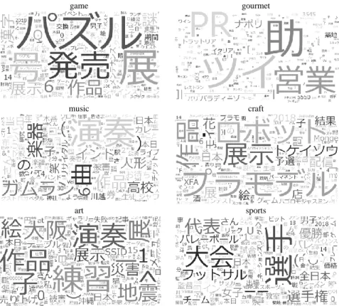
Fig. 12 shows the word clouds of each hobby category that
20 25 30 35 40 45 50 3 4 5 6 7 8 9 10 11 12 13 14 15 Accu racy (%) Number of Tweets (N) RNN LSTM GRU CNN 10 12 14 16 18 20 22 24 26 10 30 50 70 90 200 400 600 800 1000 3000 5000 7000 9000 A cc ura cy (%) Number of Features (D) Random Forests SVM 0 0.02 0.04 0.06 0.08 0.1 0.12 0.14 0.16 0.18 0.2 0% 10% 20% 30% 40% 50% 60% 70% 80% 90% 100% 1 2 3 4 5 6 7 L o ss A cc ura cy (%) Training Epoch
TrainAcc ValidationAcc Overfit TrainLoss ValLoss
game gourmet music craft art sports
game 47% 11% 12% 4% 7% 18% gourmet 11% 45% 14% 5% 10% 15% music 10% 15% 39% 10% 8% 18% craft 11% 14% 16% 40% 4% 15% art 10% 12% 14% 4% 47% 12% sports 4% 10% 10% 5% 4% 66% T rue c at egory Predicted category
game gourmet music craft art sports
game 19% 2% 14% 14% 14% 37% gourmet 0% 0% 0% 0% 0% 0% music 13% 2% 13% 18% 16% 39% craft 8% 3% 11% 16% 20% 42% art 10% 5% 20% 20% 20% 26% sports 15% 3% 11% 16% 14% 42% Predicted category T rue c at egory
were made by using feature selection based on the chi square value. The number of feature is set as 100 (only nouns were
mapped in the word clouds). More characteristic words as feature are indicated in larger font.
game gourmet
music craft
art sports
Fig. 12. Word cloud which made from selected features by χ2 value for each category.
As seen in the figure, the feature “work” frequently appeared in any categories of “game,” “music,” “craft,” and “art.” On the other hand, the features “athlete,” “championship,” “all Japan” in the category of “sports”, and the features “Naples,” “restaurant” and “wine” in the category of “gourmet” are characteristic words for each category. Therefore, it seems that accuracies in the category of “sports” and “gourmet” became higher than those in other categories.
V. CONCLUSIONS
In this paper, we proposed a method to estimate the hobby category by neural networks which use the sequential tweets of Twitter users as a training feature. As the results of the proposed methods based on four types of networks (RNN, LSTM, GRU, CNN) using word embedding feature and the baseline methods based on RF and SVM using the Bag of Words feature, the maximum accuracy was obtained by the proposed method which using LSTM when the number of tweets is six.
The category “gourmet” achieved the highest F1-score. On the other hand, we found users whose category estimation accuracy was 0%. When we analyzed this result, we found that among the users whose hobby category could not be estimated from their multiple, sequential tweets on Twitter, the contents of the tweets were not related to the hobby category described in their profile. We believe we can improve the results by collecting the users’ timelines and collecting the tweets which were posted close to the time their profile was last updated.
In the future, we would like to try to improve the accuracy
by collecting a selection of tweets based on the similarity between the profile contents and the tweet contents. And, we would like to create a distributed representation which is more suitable for their hobby category estimation by including additional training with tweets in the training data.
REFERENCES [1] Twpro. [Online]. Available: https://twpro.jp/
[2] J. Li, A. Ritter, and E. Hovy, “Weakly supervised user profile extraction from Twitter,” in Proc. the 52nd Annual Meeting of the
Association for Computational Linguistics, 2014, pp. 165-174.
[3] M. Yu, X. Han, X. Gou, J. Yu, F. Lv, and J. Li, “Content-based social network user interest tag extraction,” International Journal of
Database Theory and Application, vol. 8, no. 2, pp. 107-118, 2015.
[4] T. Forss, S. Liu, and K.-M. Bjork, “Extracting people’s hobby and interest information from social media content,” Terminology and
Knowledge Engineering 2014, Berlin, Germany, 2014.
[5] Y. Lewenberg, Y. Bachrach, and S. Volkova, “Using emotions to predict user interest areas in online social networks,” in Proc. IEEE
International Conference on Data Science and Advanced Analytics
(DSAA), 2015, pp. 1-10.
[6] A. Agarwal, O. Rambow, and N. Bhardwaj, “Predicting interests of people on online social networks,” in Proc. International Conference
on Computational Science and Engineering, Vancouver, BC, 2009, pp.
735-740.
[7] L. B. Krithika, “Finding user personal interests by tweet-mining using advanced machine learning algorithm in R,” in Proc. IOP Conf. Series:
Materials Science and Engineering, vol. 263, 2017, pp. 1-9.
[8] R. Makki, A. J. Soto, and S. Brooks, “Twitter message recommendation based on user interest profiles,” in Proc. IEEE/ACM
International Conference on Advances in Social Networks Analysis and Mining (ASONAM), 2016.
[9] N. Mangal, S. Kanwar, and R. Niyogi, “Prediction of Twitter users’ interest based on tweets,” in Proc. the First International Conference
on Intelligent Computing and Communication, pp. 167-175, 2016.
[10] S. Volkova, Y. Bachrach, and B. V. Durme, “Mining user interests to predict perceived psycho-demographic traits on Twitter,” in Proc.
IEEE Second International Conference on Big Data Computing Service and Applications (Big Data Service), 2016.
[11] P. Kapanipathi, P. Jain, C. Venkataramani, and A. Sheth, “User interests identification on Twitter using a hierarchical knowledge base,” in Proc. the Semantic Web: Trends and Challenges: 11th International
Conference, ESWC 2014, 2014, pp. 99-113.
[12] K. Watanabe and S. Kato, “Tweet recommendation system reflecting user preference based on latent dirichlet allocation and collaborative filtering,” in Proc. the 28th Annual Conference of the Japanese Society
for Artificial Intelligence, 2014, pp. 1-4.
[13] K. Kamijo, T. Natsukawa, and H. Kitamura, “Personality estimation from Japanese text,” in Proc. the Workshop on Computational
Modeling of People’s Opinions, Personality, and Emotions in Social Media, 2016, pp. 101–109.
[14] K. Matsumoto, S. Tanaka, M. Yoshida, K. Kita, and F. Ren, “Ego-state estimation from short texts based on sentence distributed representation,” International Journal of Advanced Intelligence (IJAI), vol. 9, no. 2, pp. 145-161, 2017.
[15] R. Kato, K. Nakamura, Y. Yamamoto, S. Tanaka, and K. Sakamoto, “Research for reasoning users’ attributes and habitual behavior of microblog,” IPSJ Journal, vol. 57, no. 5, pp. 1421-1435, 2016. [16] K. Ikeda, G. Hattori, K. Matsumoto, C. Ono, and T. Higashino,
“Demographic estimation of Twitter users for marketing analysis,”
IPSJ Journal Consumer Device & System (CDS), vol. 2, no. 1, pp.
82-93, 2012.
[17] D. Rao, D. Yarowsky, A. Shreevats, and M. Gupta, “Classifying latent user attributes in Twitter,” in Proc. the 2nd International Workshop on
Search and Mining User-Generated Contents, 2010, pp. 37-44.
[18] L. Sloan, J. Morgan, P. Burnap, and M. Williams, “Who tweets? Deriving the demographic characteristics of age, occupation and social class from Twitter user meta-data,” PLOS ONE, vol. 10, no. 3, pp. 1-20, 2015.
[19] M. D. A. Praveena and B. Bharathi, “A survey paper on big data analytics,” in Proc. International Conference on Information
Communication and Embedded Systems (ICICES), 2017.
[20] F. Ren and K. Matsumoto, Emotion Analysis on Social Big Data, vol. 15, no. S2, pp. 30-37, 2017.
[21] M. A. Magumba, P. Nabende, and E. Mwebaze, “Ontology boosted deep learning for disease name extraction from Twitter messages,”
Journal of Big Data, vol. 5, no. 31, pp. 1-9, 2018.
[22] M. K. Danthala, “Tweet analysis: Twitter data processing using Apache Hadoop,” International Journal of Core Engineering &
Management (IJCEM), vol. 1, issue 11, 2015.
[23] D. Sehgal and A. K. Agarwal, “Sentiment analysis of big data applications using Twitter data with the help of Hadoop framework,” in
Proc. the International Conference System Modeling & Advancement in Research Trends (SMART), 2016.
[24] M. Kumar and A. Bala, “Analyzing Twitter sentiments through big data,” in Proc. the 3rd International Conference on Computing for
Sustainable Global Development (INDIACom), 2016.
[25] R. Vatrapu, R. R. Mukkamala, A. Hussain, and B. Flesch, “Social set analysis: a set theoretical approach to big data analytics,” IEEE Access, vol. 4, pp. 2542-2571, 2016.
[26] S. Sohangir, D. Wang, A. Pomeranets, and T. M. Khoshgoftaar, “Big data: deep learning for financial sentiment analysis,” Journal of Big
Data, vol. 5, no. 3, pp. 1-25, 2018.
[27] Twpro API. [Online]. Available: https://twpro.jp/doc/api/search [28] Twitter API. [Online]. Available: https://apps.twitter.com/ [29] Tweepy. [Online]. Available: http://www.tweepy.org/
[30] Word2Vec. [Online]. Available: https://github.com/dav/word2vec [31] T. Mikolov, K. Chen, G. Corrado, and J. Dean, “Efficient estimation of
word representations in Vector Space”.
[32] J. Pennington, R. Socher, and C. D. Manning, “GloVe: Global vectors for word representation,” in Proc. the 2014 Conference on Empirical
Methods in Natural Language Processing (EMNLP), 2014, pp.
1532–1543.
[33] Pre-trained word vectors. [Online]. Available: https://github.com/facebookresearch/fastText/blob/master/pretrained-vectors.md
[34] A. Joulin, E. Grave, P. Bojanowski, and T. Mikolov, “Bag of tricks for efficient text classification,” in Proc. the 15th Conference of the
European Chapter of the Association for Computational Linguistics,
vol. 2, 2017, pp. 427–431.
[35] MeCab: Yet another part-of-speech and morphological analyzer. [Online]. Available: http://taku910.github.io/mecab/
[36] S. Hochreiter and J. Schmidhuber, “Long short-term memory,” Neural
Computation, vol. 9, no. 8, pp. 1735-1780, 1997.
[37] K. Cho, D. Bahdanau, F. Bougares, H. Schwenk, and Y. Bengio, “Learning phrase representation using RNN encoder-decoder for statistical machine translation,” in Proc. the 2014 Conference on
Empirical Methods in Natural Language Processing (EMNLP), 2014,
pp. 1724–1734.
[38] Y. LeCunn, Y. Bengio, and G. Hinton, “Deep learning,” Nature, vol. 521, pp. 436-444, 2015.
[39] D. Kingma and J. Ba, “Adam: A method for stochastic optimization,” in Proc. the 3rd International Conference for Learning
Representations, 2015.
[40] Keras. [Online]. Available: https://keras.io/
[41] TensorFlow. [Online]. Available: https://www.tensorflow.org/ [42] L. Breiman, “Random forests,” Machine Learning, vol. 45, issue 1, pp.
5-32, 2001.
[43] V. Vapnik, and A. Lerner, “Pattern recognition using generalized portrait method,” Automation and Remote Control, vol. 24, 1963. [44] Y. Yang, and J. Pedersen, “A comparative study on feature selection in
text categorization,” in Proc. the Fourteenth International Conference
on Machine Learning (ICML'97), 1997, pp. 412-420.
[45] Schikit-learn. [Online]. Available: http://scikit-learn.org
Koji Bando received the B.E. degree from
Tokushima University, Tokushima, Japan, in 1977. After graduation in 1977, He joined NTT Corporation, and currently he is president & CEO of NTT Plala Inc., Tokyo, Japan. In 2003, he received telecommunications association's IT business encouragement special award. From 2018, he is also in a doctral course of Tokushima University. His research interest includes information retrieval, natural language processing and artificial intelligence.
Kazuyuki Matsumoto received the PhD degree in
2008 from Tokushima University. He is currently an assistant professor of Tokushima University. His research interests include affective computing, emotion recognition, artificial intelligence and natural language processing. He is a member of IPSJ, ANLP, IEICE, JSAI, and IEEJ.
Minoru Yoshida is a lecturer at the Department of
Information Science and Intelligent Systems, University of Tokushima. After receiving his BSc, MSc, and PhD degrees from the University of Tokyo in 1998, 2000, and 2003, respectively, he worked as an assistant professor at the Information Technology Center, University of Tokyo. His current research interests include web document analysis and text mining for the documents on the WWW.
Kenji Kita received the B.S. degree in mathematics
and the PhD degree in electrical engineering, both from Waseda University, Tokyo, Japan, in 1981 and 1992, respectively. From 1983 to 1987, he worked for the Oki Electric Industry Co. Ltd., Tokyo, Japan. From 1987 to 1992, he was a researcher at ATR Interpreting Telephony Research Laboratories, Kyoto, Japan. Since 1992, he has been with Tokushima University, Tokushima, Japan, where he is currently a professor at the Faculty of Engineering. His current research interests include multimedia information retrieval, natural language processing, and speech recognition.