東北大学機関リポジトリTOUR

(1)

Homomorphism, and Constraint Satisfaction

著者

Hatanaka Tatsuhiko

学位授与機関

Tohoku University

学位授与番号

11301甲第18762号

(2)

Reconfiguration Problems for Graph Coloring,

Homomorphism, and Constraint Satisfaction

by

Tatsuhiko Hatanaka

Submitted to

Department of System Information Sciences

in partial fulfillment of the requirements for the degree of

Doctor of Philosophy (Information Science)

Graduate School of Information Sciences

Tohoku University, Japan

(3)

(4)

i

Acknowledgements

First of all, I would like to express my deep gratitude for my supervisor Professor Xiao Zhou. He gave me a really large amount of worthful advices and suggestions, and oﬀered a very comfortable place that made my life of research so pleasant. Without his continual help and encouragement, this thesis would not be completed. I am really grateful to my thesis advisor, Associate Professor Takehiro Ito. He also helped me on the presentations and on the writing style of my papers, and gave me a lot of opportunities to build up my career as a researcher. Without his numerous number of helpful discussions and supports, this thesis would not be completed.

I would also like to show my special thanks to the other members of my graduate committee, Professor Takeshi Tokuyama and Professor Ayumi Shinohara, for their insightful suggestions and comments.

Furthermore, I would also like to thank Assistant Professor Akira Suzuki for his many suggestions and guidance, and for many things. All of his useful suggestions on my research and his kind help in everyday life have been invaluable to me.

Finally, I would like to acknowledge with sincere thanks the all-out cooperation and services rendered by the members of Algorithm Theory Laboratory for many things.

(5)

Abstract

Since the 2000s, the framework of (combinatorial) reconfiguration has been exten-sively studied in the field of theoretical computer science. This framework models several “dynamic” situations where we wish to find a step-by-step transformation between two feasible solutions of a combinatorial search problem such that all in-termediate solutions are also feasible and each step respects a fixed reconfiguration rule. This reconfiguration framework has been applied to several well-studied com-binatorial search problems. In this thesis, we mainly study the reconfiguration problem for the well-known constraint satisfaction problem (CSP), which is a gener-alization of several combinatorial search problems including graph coloring, Boolean satisfiability, graph homomorphism and so on. In CSP, we are asked to find an as-signment of values to given variables so as to satisfy all of given constraints. In the reconfiguration problem for CSP, we are given an instance of CSP together with its two satisfying assignments, and asked to determine whether one assignment can be transformed into the other by changing a single variable assignment at a time, while always remaining satisfying assignment. We also study several special cases of the problem, especially the reconfiguration problems for graph coloring, graph homo-morphism, and their list variants. In this thesis, we study these problems from the viewpoints of polynomial-time solvability and parameterized complexity, and give several interesting boundaries of tractable and intractable cases.

(6)

iii

List of Figures

1.1 The 15-puzzle. Each placement of blocks is feasible and only one block is slid in each step. . . . 2 1.2 A transformation of 4-colorings. A vertex which is recolored from the

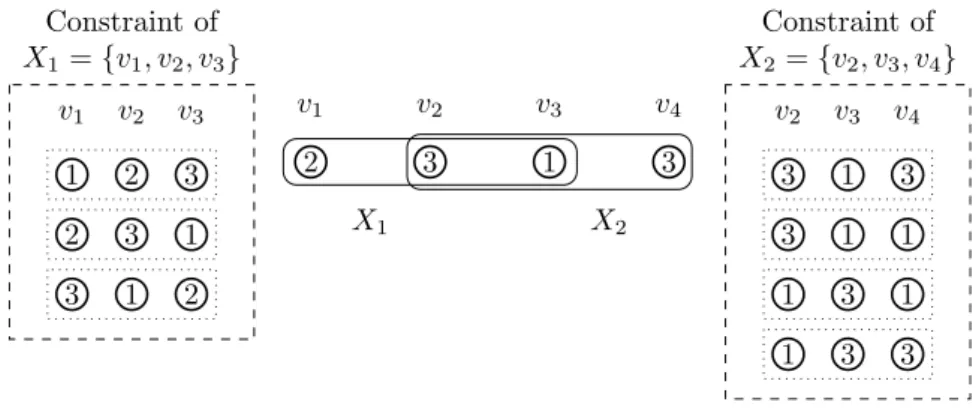
previous 4-coloring is depicted by a thick circle. . . . 3 1.3 An example of constraints which represent allowed assignments to the

vertices in CSP (left and right of the figure) and a mapping which satisfies all constraints (middle of the figure). . . . 5 1.4 (a) Relationships between problems. Each dotted line between P

(lower) and Q (upper) means that P is a special case of Q. (b) Re-lationships between graph parameters. cw, mw, tw, pw, td, vc, bw and n are the cliquewidth, the modular-width, the treewidth, the pathwidth, the tree-depth, the size of a minimum vertex cover, the bandwidth and the number of vertices of a graph, respectively. Each arrow α → β means that α is stronger than β, that is, if α is bounded by a constant then β is also bounded by some constant. . . . 7 1.5 _{Known and our results for CR with respect to graph classes. Each}

arrow A → B represents that the graph class B is a subclass of the graph class A. . . 10 1.6 _{Known and our results for LCR with respect to graph classes. Each}

arrow A → B represents that the graph class B is a subclass of the graph class A. . . 10

(11)

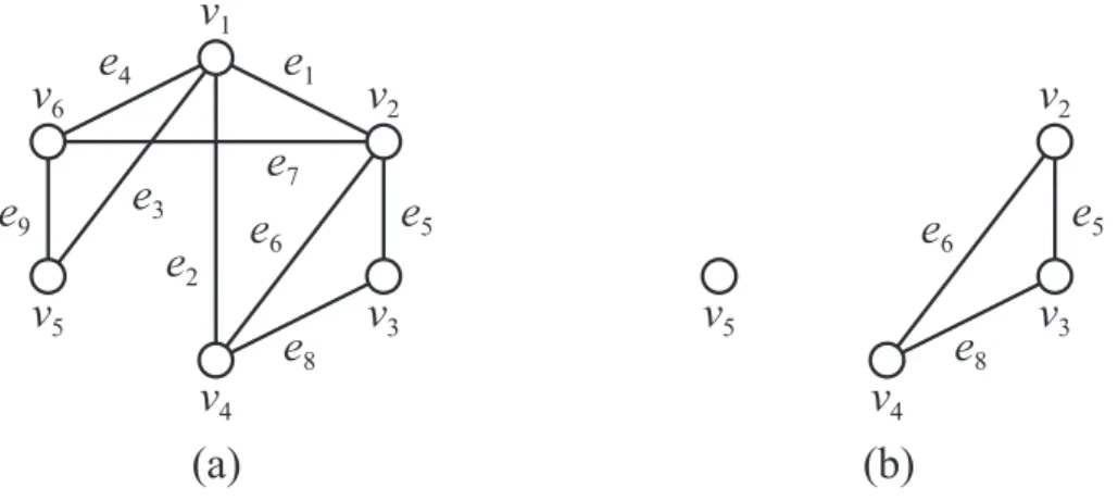
2.1 (a) A graph G with six vertices and nine edges, and (b) a subgraph

G′ of G induced by a vertex set V′ ={v2, v3, v4, v5}. . . 15

2.2 A hypergraph G and the subhypergraph G[{v2, v3, v4}] induced by {v2, v3, v4}. . . 16

2.3 (a) A graph G, (b) the contraction of {v2, v3} ⊆ V (G), and (c) the complement of G. . . 18

2.4 An example of the breadth-first search of th graph in Figure 2.1(a). . 18

2.5 Two isomorphic graphs. . . . 19

2.6 Two isomorphic hypergraphs G and G′ under the bijections ϕ and π. 19 2.7 (a) A rooted tree with the root v1, and (b) the rooted subtree with the root v4. . . 20

2.8 A spanning tree of the graph in Figure 2.1(a). . . 21

2.9 (a) A graph G, and (b) its path decomposition. In (b), each graph surrounded by dotted box is the graph induced each subset. . . . 22

2.10 Examples of (a) a module and (b) a prime. . . 22

2.11 An example of substitution operation. . . 23

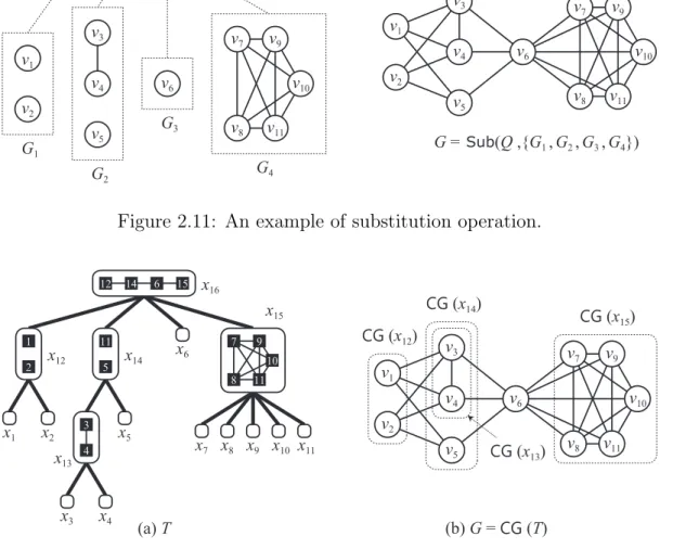
2.12 (a) A substitution tree T for (b) a graph G. . . 23

2.13 An example of the replacement described in the proof of Proposition 2.1. 25 2.14 A graph G, a graph H whose vertex set is {1, 2, 3, 4}, and a homo-morphism from f from G to H. . . 30

2.15 (a) An instanceI = (G, {1, 2, 3}, C) of constraint satisfiability, and (b) the solution graphS (I). . . 33

3.1 Example for frozen vertices: The upper three vertices are frozen on fs and ftbecause they form a clique of size three, and their lists contain only three colors in total. . . 37

(12)

ix

3.3 (a) A graph H′, a list L and an L-coloring gs, and (b) a constructed

graph G and k-coloring fs. . . 39

3.4 An example of a split graph, whose vertex set can be partitioned into a clique VQ and an independent set VI. . . 43

3.5 (a) A trivially perfect graph, and (b) its corresponding cotree. . . 44 4.1 A caterpillar G and its vertex ordering, where the subgraph

sur-rounded by a dotted rectangle corresponds to G8. . . 50

4.2 (a) A graph G and a list L, and (b) the reconfiguration graph RL

G. . . 52

4.3 (a) A caterpillar G = G4, (b) the reconfiguration graph R4 consisting

of all L-colorings of G, and (c) the encoding graph H4of Rs4 consisting

of two e-nodes x and y, where each L-coloring in (b) is represented as the sequence of colors assigned to the vertices in G from left to right. 55 4.4 The graph Gi for (a) vi ∈ VL and (b) vi ∈ VS. . . 57

4.5 Application of our algorithm to the instance depicted in (a)–(c). In (d)–(h), coli(x) ∈ L(sp(i)) is attached to each node x, and the

e-nodes x with inii(x) = 1 and tari(x) = 1 have the labels “ini” and

“tar,” respectively. Furthermore, in (e), (f) and (h), the small graph contained in each e-node x of Hi represents the subgraph of Hi−1

induced by EN(x). . . . 58

4.6 The path P with n vertices. . . 68

5.1 (a) A directed graph R and (b) the edge set Ep between Lp and Lp+1. 70

7.1 (a) An instance H of independent set, and (b) the

graph G and the list L. The set Vfor contains

ver-tices of (i, j; p, q)-forbidding gadgets for all (i, j) ∈

{(1, 2), (1, 3), (2, 3)} and all (p, q) ∈ {(1, 1), (2, 2), (3, 3), (4, 4), (5, 5),

(13)

8.1 An example of two subhypergraphs H1 and H2 of G which satisfies

the conditions (1) and (2). We draw each hyperedge of size two as a solid line, and omit the bijection π : E(H₁′) → E(H₂′) since it is uniquely defined from ϕ : V (H₁′) → V (H₂′). If A and C satisfy the conditions (3) and (4), H1 and H2 are identical. . . 85

8.2 An example of an application of our algorithm. We first focus on x8,

which is a parallel node whose children are already kernelized, and find thatM1(x1) = M1(x2) holds. Therefore, we delete CG(x1) from

the input graph. Then, x8 has only one child, and hence we contract

the edge x8x9 in order to maintain being a PMD-tree. We next focus

on x11 and find that M2(x9) = M2(x10) holds. We thus remove

CG(x10) from the current graph and fixing a PMD-tree. Then, the

algorithm terminates because we have processed all parallel nodes. . . 94 9.1 A graph G and a tree-depth decomposition T of G with the root v1. . 99

9.2 (a) An instance J = (G, {0, 1}, C) and (b) the implication graph IMP(J ) for J . . . 115

(14)

1

Chapter 1 Introduction

1.1 Combinatorial reconfiguration

Since the 2000s, the framework of (combinatorial ) reconfiguration [34] has been extensively studied in the field of theoretical computer science. (See surveys [38, 50, 33].) This framework models several “dynamic” situations where we wish to find a step-by-step transformation between two feasible states such that all intermediate states are also feasible and each step respects a fixed reconfiguration rule. For example, sliding block puzzles [32] such as the 15-puzzle (see Figure 1.1) can be captured in this framework; the feasible states are placements of rectangle blocks in a rectangle frame without an overlap, and a reconfiguration rule is sliding exactly one block to an empty cell at a time. As another example, consider the situation where frequency channels are assigned to base stations so that no interference occurs. Assume now that the current feasible assignment must be transformed (e.g., to use a newly found better assignment or to satisfy new side constraints), while maintaining the feasibility (so that the users receive service even during the transformation). This problem can also be modeled in the reconfiguration framework; the feasible states are feasible frequency assignments, and a reconfiguration rule may be reassigning a frequency channel of a single base station.

Generally, a (combinatorial ) reconfiguration problem can be considered as a prob-lem asking the reachability of two vertices in a solution graph (also called a

reconfig-uration graph) defined as follows. The vertex set of a solution graph corresponds to

(15)

1 2 3 4 5 6 7 8 9 10 11 13 14 15 12 1 2 3 4 5 6 7 8 9 10 11 13 14 15 12 1 2 3 4 5 6 7 8 9 10 11 12 13 14 15

Figure 1.1: The 15-puzzle. Each placement of blocks is feasible and only one block is slid in each step.

feasible states may often be defined as a set of feasible solutions for an instance of a (combinatorial) search problem. Indeed, several reconfiguration problems based on search problems are studied well, such as Boolean satisfiability reconfigu-ration [26, 44, 47], shortest path reconfigureconfigu-ration [3, 40], independent set reconfiguration [5, 21, 32, 41, 42], vertex cover reconfiguration [37, 48], dominating set reconfiguration [28, 30].

As a concrete example of such reconfiguration problems, we here introduce the (vertex) coloring reconfiguration problem [4, 7, 17, 60], which is one of the most well-studied reconfiguration problems. (See Figure 1.2 for example.) Let

G = (V, E) be a graph and let C be a set of k colors. A k-coloring (or simply

a vertex coloring) of G is a mapping f : V → C such that f(v) ̸= f(w) holds for every edge vw ∈ E. In coloring reconfiguration, the vertex set of a solution graph is the set of all k-colorings of G, and two vertices f and f′ are adjacent in the

solution graph if f′ is obtained from f by changing the color assignment on a single

vertex, and vice versa. Then, for a given graph G, a color set C of size k, and two

k-colorings fs and ft of G, the problem asks whether there exists a walk between

fs and ft in the solution graph for G and C; such a walk is called a reconfiguration

(16)

1.2 Applications 3 2 1 4 3 2 3 4 3 2 3 1 3 2 3 1 4

Figure 1.2: A transformation of 4-colorings. A vertex which is recolored from the previous 4-coloring is depicted by a thick circle.

1.2 Applications

The framework of reconfiguration has many applications as the “feasibility” is preserved during the transformation.

1.2.1 Dynamic transformation of system configurations

Recall the transformation of frequency assignments, which we presented in the beginning of the chapter. Actually, this problem can be modeled by coloring reconfiguration if we consider each base station as a vertex, and each frequency channel as a color, and joining each pair of two base stations which have the high potential of interference. Notice that a frequency assignment without interference corresponds to a k-coloring, and reassigning a frequency channel on a single base station corresponds to changing the color assignment on a single vertex. Similar situations may occur when we wish to dynamically transform a configuration of a system into another one while maintaining the feasibility. Another example is power supply reconfiguration [34], which models the switching of the power supply routing between power stations and customers. Thus, the reconfiguration framework can be applied to several practical issues.

1.2.2 Feedback to search problems

We here note that a research on a reconfiguration problem may provide us a deeper understanding of the “solution space” of the corresponding search problem, since we deal not only with the existence of solutions but also with the relationship

(17)

between them. Thus, sometimes it brings a good feedback to the search problem. For example, Wrochna [12] gave another (much shorter) proof of the theorem that any graph without a cycle of length dividable by three has a 3-coloring, which was originally proved by Chen and Saito [18] in 1994, using ideas provided to solve 3-coloring reconfiguration [17]. Roughly speaking, the proof uses the fact that the reconfiguration preserves the feasibility.

1.3 Problems studied in this thesis

In this thesis, we mainly study (list) coloring reconfiguration, (list) homomorphism reconfiguration, and constraint satisfiability recon-figuration from the viewpoints of polynomial-time solvability and parameterized complexity. The formal definitions of the problems will be given in Chapter 2, but we here briefly introduce them.

List coloring reconfiguration is a generalization of coloring reconfig-uration where we are given a list of allowed colors for each vertex as an additional input and feasible solutions are k-colorings which respect all lists. (List) homo-morphism reconfiguration is a generalization of (list) coloring reconfig-uration defined as follows. In addition to a color set, we are also given a set of pairs of colors which can be assigned to adjacent vertices in G. This is represented by a graph H which has C as the vertex set and the set of pairs as the edge set, called an underlying graph.1 Then, feasible solutions are k-colorings which respect the edge set H (and all lists). We note that (List) homomorphism reconfiguration is equivalent to (list) coloring reconfiguration when an underlying graph H is a complete graph.

Constraint satisfiability reconfiguration is the reconfiguration problem

1 _{In this thesis, we only consider simple undirected underlying graphs unless otherwise}

stated, although loops and/or directed edges are often allowed in the literature of graph homomorphisms.

(18)

1.3 Problems studied in this thesis 5 2 v1 3 v2 1 v3 3 v4 X1 X2 Constraint of X1= {v1, v2, v3} v1 v2 v3 1 2 3 2 3 1 3 1 2 Constraint of X2= {v2, v3, v4} v2 v3 v4 3 1 3 3 1 1 1 3 1 1 3 3

Figure 1.3: An example of constraints which represent allowed assignments to the vertices in CSP (left and right of the figure) and a mapping which satisfies all constraints (middle of the figure).

for well-known constraint satisfaction problem (CSP, for short), which is a general-ization of several combinatorial problems including vertex coloring, Boolean satisfi-ability, graph homomorphism and so on. In this thesis, we formulate them by means of hypergraphs. Let G = (V, E) be a hypergraph. Let D be a set, called a domain; each element of D is called a value and we always denote by k the size of a domain. In CSP, each hyperedge X ∈ E has a constraint which represents the values allowed to be assigned to the vertices in X at the same time, and we wish to find a mapping

f : V → D which satisfies the constraints of all hyperedges in G. (See Figure 1.3

for an example.) For example, in the case of vertex coloring, we can see that every hyperedge consists of two vertices, and has the common constraint that any two diﬀerent colors can be assigned to the two vertices in the hyperedge at the same time. In constraint satisfiability reconfiguration, feasible solutions are mappings satisfying all constraints, and the reconfiguration rule is changing a value of a single vertex at a time. Boolean constraint satisfiability is the special case of constraint satisfiability where |D| = 2. For an integer r ≥ 1, r-ary constraint satisfiability is the special case of constraint satisfiability where all hyperedges have size at most r.

(19)

reconfigura-tion includes several reconfigurareconfigura-tion problems as special cases such as Boolean constraint satisfiability reconfiguration, r-ary constraint satisfia-bility reconfiguration, (list) homomorphism reconfiguration, (list) coloring reconfiguration. In the remainder of the thesis, we use the following abbreviations:

• CSR for constraint satisfiability reconfiguration;

• BCSR for Boolean constraint satisfiability reconfiguration; • r-CSR for r-ary constraint satisfiability reconfiguration for each

integer r≥ 1;

• (L)HR for (list) homomorphism reconfiguration; and • (L)CR for (list) coloring reconfiguration.

Relationships between problems are illustrated in Figure 1.4(a).

1.4 Known and related results

There are many literatures which study special cases of CSR (including (L)CR and (L)HR) and their shortest variants. In the shortest variant, we are given an instance with an integer ℓ ≥ 0, and asked whether there exists a reconfiguration sequence of length at most ℓ. We here state only the results from the viewpoint of the computational complexity.

One of the most well-studied special cases of CSR is BCSR [6, 14, 26, 43, 44, 47, 57]. Gopalan et al. [26] gave a computational dichotomy for BCSR with re-spect to a set S of logical relations which can be used to define each constraint: the problem is PSPACE-complete or in P for each fixed S. In addition, Cardinal et al. [14] showed that the problem remains PSPACE-complete even if S is equiva-lent to monotone Not-All-Equal 3-SAT (i.e., each constraint is a set of surjections)

(20)

1.4 Known and related results 7 CSR BCSR 3-CSR 2-CSR LHR LCR HR CR (a) cw mw tw pw bw td vc n (b)

Figure 1.4: (a) Relationships between problems. Each dotted line between P (lower) and Q (upper) means that P is a special case of Q. (b) Relationships between graph parameters. cw, mw, tw, pw, td, vc, bw and n are the cliquewidth, the modular-width, the treemodular-width, the pathmodular-width, the tree-depth, the size of a minimum vertex cover, the bandwidth and the number of vertices of a graph, respectively. Each arrow α→ β means that α is stronger than β, that is, if α is bounded by a constant then β is also bounded by some constant.

and a “variable-clause incidence graph” is planar. For the shortest variant, a com-putational trichotomy is known: Mouawad et al. [47] proved that the problem is PSPACE-complete, NP-complete or in P for each fixed S. Bonsma et al. [6] proved that the shortest variant is W [2]-hard when parameterized by ℓ even if S is equiva-lent to Horn SAT.

Another well-studied spacial case is CR [1, 2, 4, 6, 7, 8, 15, 16, 17, 23, 24, 27, 39, 51, 52, 60]. This problem is PSPACE-complete for k ≥ 4 and bipartite planar graphs [4] but in P for k ≤ 3 [17]. The second tractability result is extended to the shortest variant [39], and even can be applied to LCR. Moreover, it is known that the problem remains PSPACE-complete even if k is a fixed constant for line graphs (for any fixed k ≥ 5) [52] and for bounded bandwidth graphs [60]. On the other hand, there exists a polynomial-time algorithm for (k− 2)-connected chordal

(21)

graphs [7]. For the shortest variant parameterized by ℓ, some intractability results are known; it is W [1]-hard [6] and does not admit a polynomial kernelization when

k is fixed unless the polynomial hierarchy collapses [39]. As a generalization of CR,

LCR is also studied [36, 52, 60]. The problem is PSPACE-complete even for graphs with pathwidth two and constant bandwidth and some constant k [60] and for line graphs and any fixed k≥ 4 [52].

HR is also well-studied as a generalization of CR. Several literatures investigated HR from the viewpoint of graph classes in which a given graph G or an underlying graph H lies [11, 10, 12, 13, 59, 60]. Brewster et al. [12] gave a dichotomy for a special case of HR in which H is a (p, q)-circular clique; it is PSPACE-complete if

p/q ≥ 4 but is in P otherwise. We note that this result generalizes the complexity

of CR with respect to k, since a complete graph Kk with k vertices is a (k,

1)-circular clique. It is also known that the problem is PSPACE-complete even if (a)

H is an odd wheel [10] or (b) H is some fixed graph and G is a cycle [60]. On the

other hand, it can be solved in polynomial time if G is a tree [60] or H contains no cycles of length four [59]. Furthermore, a fixed-parameter algorithm is known when parameterized by k + td [60]; note that it can be easily extended for LHR.

Finally, we refer to the shortest variant of CSR. Bonsma et al. [6] gave a fixed-parameter algorithm for the shortest variant fixed-parameterized by k + r + ℓ, where r is the maximum size of a hyperedge. This implies that shortest variants of BCSR and 2-CSR are fixed-parameter tractable when parameterized by r + ℓ and k + ℓ, respectively. They also showed that the problem is intractable in general if at least one of {k, r, ℓ} is excluded from the parameter.

1.5 Our contribution

In this thesis, we investigate the complexity of CSR and its spacial cases, espe-cially 3-CSR, 2-CSR, (L)HR and (L)CR, from the viewpoints of polynomial-time

(22)

1.5 Our contribution 9

Table 1.1: Computational complexities with respect to the size k of a domain.

k ≥ 4 k = 3 k = 2

CSR PSPACE-c. PSPACE-c. PSPACE-c.

3-CSR PSPACE-c. PSPACE-c. PSPACE-c. [26]

2-CSR PSPACE-c. PSPACE-c. [Thm. 6.1] P [Thm. 6.2]

LHR PSPACE-c. P [Thm. 5.2] P

LCR PSPACE-c. P [17] P

HR PSPACE-c. P [59] P

CR PSPACE-c. [4] P P

solvability and parameterized complexity, and give several interesting boundaries of tractable and intractable cases.

1.5.1 Polynomial-time solvability

We first classify the complexity of the problems for each fixed size k of a domain; we note that k corresponds to the number of colors in (L)CR and (L)HR. Together with known results, our results give interesting boundaries of (in)tractability as summarized in Table 1.1. In particular, our results unravel the boundaries with respect to k for 2-CSR and LHR. The other interesting contrast we show is the boundary between 2-CSR and LHR for k = 3.

In order to give more detailed analyses, we also focus on the structure of an input (hyper)graph and explore the structures which make the problems hard. We first an-alyze the complexities of CR and (L)CR from the viewpoint of graph classes. (See Figures 1.5 and 1.6.) In particular, the PSPACE-completeness of LCR for chordal graphs answers the open question posed by Bonsma and Paulusma [7]. Moreover, we show the boundary of the complexity of LCR with respect to pathwidth; we give a polynomial-time algorithm for graphs with pathwidth one, while it is PSPACE-complete for graphs with pathwidth two [60]. We next investigate the complexity for graphs with pathwidth one or two of more ganeral problems, that is, (L)HR, 2-CSR, 3-CSR and CSR. (See Table 1.2.)

(23)

PSPACE-complete [Thm. 3.1] [4] [4] [Thm. 3.3] [Thm. 3.5] [Thm. 3.6] [Thm. 3.7] Open P chordal interval _q-tree trivially perfect split tree series-parallel planar 2-degenerate 3-degenerate

Figure 1.5: Known and our results for CR with respect to graph classes. Each arrow

A→ B represents that the graph class B is a subclass of the graph class A.

[60] PSPACE-complete [4] [4] [Thm. 3.2] [Thm. 4.2] [Thm. 4.1] P chordal interval threshold trivially perfect split pathwidth two pathwidth one planar cograph 2-degenerate

Figure 1.6: Known and our results for LCR with respect to graph classes. Each arrow A→ B represents that the graph class B is a subclass of the graph class A.

1.5.2 Parameterized complexity

As we stated in Section 1.4, most fixed-parameter algorithms (other than the one in [60]) known for CSR and its special cases take the length ℓ of a reconfiguration sequence as a part of the parameter. If we consider somewhat practical situations (e.g., the transformation of frequency assignments), it may be reasonable enough to wish to find a short reconfiguration sequence and thus assume a small ℓ. On the other hand, when the reconfigurability matters, this is not the case, since the

(24)

short-1.5 Our contribution 11

Table 1.2: Computational complexity for graphs with pathwidth at most two.

pw = 2 pw = 1 CSR PSPACE-c. PSPACE-c. 3-CSR PSPACE-c. PSPACE-c. 2-CSR PSPACE-c. PSPACE-c. LHR PSPACE-c. PSPACE-c. [Thm. 5.1] LCR PSPACE-c. [60] P [Thm. 4.2] HR PSPACE-c. [60] P [60] CR P [Thm. 3.3] P

est reconfiguration sequence can be arbitrarily large and even superpolynomial [4]. Therefore, we investigate the parameterized complexity for several parameters which do not contain ℓ.

One may come up with the size k of a domain as such natural parameter. How-ever, the problems are PSPACE-complete even if k is fixed even for several restricted classes, and hence fixed-parameter algorithms parameterized k never exist under P ̸= PSPACE. Thus, as other natural parameters, we consider several graph pa-rameters such as the cliquewidth cw, the modular-width mw, the treewidth tw, the pathwidth pw, the tree-depth td, the size vc of a minimum vertex cover, the band-width bw, and the number n of vertices; we again define each graph parameter of a hypergraph as that of its primal graph. The relationships between graph parameters are summarized in Figure 1.4(b); note that tractability (resp., intractability) result propagates downward (resp., upward).

We first show that HR parameterized by the number of vertices and LCR param-eterized by the size of a minimum vertex cover are both W [1]-hard. These imply that fixed-parameter algorithms are unlikely to exist for almost all graph parameters in Figure 1.4. Therefore, we take as parameters k plus several graph parameters, and summarize the known and our results in Table 1.3. We note that a fixed-parameter tractability of CSR parameterized by k + vc can be obtained as a corollary of The-orem 9.1. However, TheThe-orem 9.3 gives a faster algorithm and TheThe-orem 9.2 gives an

(25)

Table 1.3: Parameterized complexity with respect to k plus graph parameters. Parameter k + mw k + td k + vc k + bw CSR PSPACE-c. FPT FPT PSPACE-c. [Thm. 9.1] [Thms. 9.2, 9.3] 3-CSR PSPACE-c. FPT FPT PSPACE-c. 2-CSR PSPACE-c. FPT FPT PSPACE-c. [Cor. 6.1] LHR FPT [Thm. 8.1] FPT FPT PSPACE-c. LCR FPT FPT FPT PSPACE-c. HR FPT FPT [60] FPT PSPACE-c. CR FPT FPT FPT PSPACE-c. [60]

Table 1.4: Parameterized complexity with respect to k and the number nb of non-Boolean vertices. Parameter k + nb nb CSR PSPACE-c. PSPACE-c. 3-CSR PSPACE-c. [26] PSPACE-c. 2-CSR FPT [Thm. 9.5] W [1]-hard but XP [Thm. 9.5] LHR FPT W [1]-hard but XP LCR FPT W [1]-hard but XP

HR FPT W [1]-hard [Cor. 7.1] but XP

CR FPT FPT [Pro. 9.3]

algorithm for the shortest variant.

We next consider another parameter which is not graph-structural, that is, the number nb of “non-Boolean vertices”, in order to extend the analysis for k = 2 presented in the previous section. Roughly speaking, nb reflects how an instance is close to that of BCSR. The parameterized complexity regarding nb is summarized in Table 1.4. We note that k = 2 implies that nb = 0, and hence the algorithm given in Theorem 9.5 generalizes Theorem 6.2. Therefore, this result gives a more detailed boundary of the complexity of 2-CSR between k = 3 and k = 2.

Finally, we prove that 2-CSR cannot be solved in time O∗((k + n)o(k+n)_{) under}

the exponential time hypothesis (ETH). This lower bound matches the running time shown in Theorems 2.1, 9.3 and 9.5, respectively.

(26)

1.6 Organization of this thesis 13

1.6 Organization of this thesis

The main part of this thesis consists of two parts; each part is divided into chapters according to the target problem.

(b)

Figure 2.1: (a) A graph G with six vertices and nine edges, and (b) a subgraph G′ of G induced by a vertex set V′ ={v2, v3, v4, v5}.

where each vertex is drawn as a circle together with its index and each edge is drawn as a line joining two circles (vertices) together with its index. If e = vw is an edge, then we say that e joins v and w; e is incident to v and w; v and w are

adjacent (by the edge e;) and w is a neighbor of v. In the graph in Figure 2.1(a),

for example, e3 joins v1 and v5; e7 is incident to v2 and v6; v1 and v2 are adjacent

by e1; and v3 is a neighbor of v4. The neighborhood N (G, v) of a vertex v is a set

of all neighbors of v, that is, N (G, v) = {w ∈ V (G) | vw ∈ E(G)}. For a vertex subset V′ ⊆ V (G), we denote N(G, V′) := ∪_v_∈V′N (G, v)\ V′. The degree d(G, v) of a vertex v is the size (the cardinality) of the neighborhood N (G, v) of v. In the graph in Figure 2.1(a), N (G, v6) ={v1, v2, v5} and hence d(G, v6) = 3.

A subgraph of a graph G = (V, E) is a graph G′ = (V′, E′) such that V′ ⊆ V and

E′ ⊆ E; we denote G′ ⊆ G and say that G contains G′. If E′ is equal to the set of all the edges of G that join vertices in V′, that is, E′ ={vw ∈ E | v, w ∈ V′∧ v ̸= w}, then G′ is called the subgraph induced by V′ or simply called the induced subgraph;

we denote G′ = G[V′]. Figure 2.1(b) depicts a subgraph G′ of G in Figure 2.1(a)

induced by a vertex set V′ ={v2, v3, v4, v5}. For an induced subgraph G′ = (V′, E′)

(29)

v1 v2 v3 v4 G X1 X2 X3 v2 v3 v4 G[{v2, v3, v4}]

Figure 2.2: A hypergraph G and the subhypergraph G[{v2, v3, v4}] induced by

{v2, v3, v4}.

2.1.2 Hypergraphs, primal graphs and subhypergraphs

A hypergraph G is a pair (V, E), where V is a set of vertices and E is a family of non-empty vertex subsets, called hyperedges. We sometimes denote by V (G) and

E(G) the vertex set and the hyperedge set of G, respectively. A hypergraph G

is r-uniform if every hyperedge consists of exactly r (≥ 1) vertices. Any simple undirected graph can be considered as a 2-uniform hypergraph and a hyperedge of size exactly two is simply called an edge. An edge {v, w} is sometimes denoted by

vw or wv for notational convenience.

Let G be a hypergraph. The primal graph P(G) of G is a graph such that

V (P(G)) = V (G) and two distinct vertices are connected by an edge if they are

contained in the same hyperedge of G. We denote N (G, v) := N (P(G), v) for any vertex v ∈ V , and N(G, V′) := N (P(G), V′) for any vertex subset V′; we say that

v is adjacent to w if w ∈ N(G, v). For a vertex subset V′ ⊆ V (G), we define the subhypergraph of G induced by V′ as the hypergraph G′ such that V (G′) = V′ and

E(G′) ={X ∩ V′: X ∈ E(G), X ∩ V′ ̸= ∅}. We denote by G[V′] the subhypergraph of G induced by V′ for any vertex subset V′. We sometimes call a hypergraph G′

an induced subhypergraph (of G) if G[V′] = G′ for some vertex subset V′ ⊆ V (G). (See Figure 2.2.) We use the notation G\ V′ to denote G[V (G)\ V′].

(30)

2.1 Basic graph-theoretical terminologies 17

2.1.3 Paths, cycles and connectivities

Let G = (V, E) be a graph. A walk from a vertex v to a vertex w is a sequenceW =

⟨v0 = v, v1, . . . , vℓ = w⟩ of vertices such that vi−1vi ∈ E for every i ∈ {1, 2, . . . , ℓ}.

The length of W is ℓ. If the vertices v1, v2,· · · , vℓ are distinct, then the walk W is

called a path. A path or walk is closed if v0 = vℓ. A closed path with length at least

one is called a cycle. In the graph in Figure 2.1(a), ⟨v1, v2, v6, v1, v4⟩ is a walk but

not a path, ⟨v2, v6, v5, v1⟩ is a path but not a cycle, and ⟨v2, v3, v4, v2⟩ is a cycle. The

distance dist(v, w) between v and w is the length of a shortest path between v and w. In the graph in Figure 2.1(a), dist(v3, v5) = 3 since ⟨v3, v4, v1, v5⟩ is a shortest

path between v3 and v5.

A graph G is connected if there is a path between v and w for any two distinct vertices v and w in G. A graph G is disconnected if it is not connected. The graph in Figure 2.1(a) is connected while the graph in Figure 2.1(b) is disconnected. Unless otherwise stated, we consider only simple connected undirected graphs. An induced subgraph G′ of G is called a connected component if there is no connected subgraph

G′′ such that G′ ⊆ G′′. In Figure 2.1(b), the subgraphs induced by{v2, v3, v4} and

{v5} are the connected components. Similarly, a hypergraph G is connected (resp.,

disconnected ) if P(G) is connected (resp., disconnected).

2.1.4 Operations on graphs

In this section, we introduce some operations on graphs which construct a new graph. Let G = (V, E) be a graph. For a vertex subset X ⊆ V which induces a connected subgraph, the contraction of X is obtaining a graph G′ = (V′, E′) from G by deleting all edges of G[X] and replacing all vertices in X with a new vertex x so that x is adjacent all neighbors of each vertex in X. Formally, V′ := (V \ X) ∪ {x} and E′ :={ϕ(v)ϕ(w) | vw ∈ E \ E(G[X])}, where ϕ is a mapping from V to V′ such that ϕ(v) = x if v ∈ X, and ϕ(v) = v otherwise. The complement G of G is a graph

(31)

3

v

4

key: v

2

Figure 2.4: An example of the breadth-first search of th graph in Figure 2.1(a).

obtained from G by reversing the adjacencies between all pairs of distinct vertices. Formally, G = (V, E) such that E ={vw | v, w ∈ V ∧ v ̸= w} \ E.

2.1.5 Breadth-first search

The breadth-first search of a graph G = (V, E) is an algorithm searching vertices of G as follows. It starts with some vertex v ∈ V and lets v the “key” vertex. Then it recursively visits all unvisited neighbors of the key vertex, and selects an arbitrary vertex which has been visited and has a unvisited neighbor as a new key. This algorithm runs in time O(|V | + |E|) [19]. Figure 2.1 shows an example of the breadth-first search starting with v5, where the visited vertices are depicted as black

(32)

2.1 Basic graph-theoretical terminologies 19 v 1 v₂ v₆ v 5 v3 v₄ u₁ u₂ u₆ u₅ u₃ u₄

Figure 2.5: Two isomorphic graphs.

v1 v2 v3 v4 G X1 X2 X3 φ(v1) φ(v3) φ(v4) φ(v2) G0 π(X1) π(X2) π(X3)

Figure 2.6: Two isomorphic hypergraphs G and G′ under the bijections ϕ and π.

2.1.6 Graph isomorphism

Two graphs G1 and G2 are isomorphic if there exists a bijective function ϕ :

V (G1) → V (G2), that is, vw ∈ E(G1) if and only if ϕ(v)ϕ(w)∈ E(G2). Figure 2.5

shows an example of two isomorphic graphs, where the bijective function maps vi

to ui for each i∈ {1, 2, 3, 4, 5, 6}.

Two hypergraphs G and G′are isomorphic if there exist two bijections ϕ : V (G)→

V (G′) and π : E(G) → E(G′) such that π(X) = {ϕ(v1), ϕ(v2), . . . , ϕ(vr)} ∈ E(G′)

holds for each hyperedge X = {v1, v2, . . . , vr} ∈ E(G). (See Figure 2.6.) Notice

that a bijection π between two hyperedge sets is uniquely determined by a bijection

ϕ between two vertex sets.

2.1.7 Independent sets, vertex covers and cliques

Let G = (V, E) be a graph. An independent set is a vertex subset V′ of V such

root v4.

cover is a vertex subset V′ of V such that V \ V′ is an independent set. We denote by vc(G) the size of a minimum vertex cover of G. A clique is a vertex subset V′

of V such that every pair of two distinct vertices v and w in V′ is adjacent. We

denote by ω(G) the maximum clique size of G. In the graph G in Figure 2.1(a),

{v3, v5} is a maximum independent set, {v1, v2, v4, v6} is a minimum vertex cover,

and {v1, v2, v6} is a maximum clique, and hence vc(G) = 4 and ω(G) = 3.

2.2 Graph paremeters and graph classes

2.2.1 Forests and trees

A forest is a graph which contains no cycle. A tree is a connected forest. A path is a tree which has at most two leaves.

A rooted tree T is a tree in which one of the vertices is distinguished from the others. The distinguished vertex is called the root of the tree. A rooted tree is usually drawn so that the root is located at the top, as illustrated in Figure 2.7(a) where v1 is the root. For each edge vw ∈ E(T ) such that dist(r, v) + 1 = dist(r, w),

we say that v is the parent of w and w is a child of v. For example, in the rooted tree in Figure 2.7(a), v4 is the parent of v6 and v7; and v6 and v7 are children of

(34)

2.2 Graph paremeters and graph classes 21

v4. A vertex v in a tree is called a leaf if it has no child. Otherwise, v is a called

an internal node. For each vertex v ∈ V (T ), the rooted subtree Tv with the root

v is a connected component of T′ = (V (T ), E(T )\ {e}) which contains v, where e joins v and v’s parent. Figure 2.7(b) depicts the rooted subtree of the rooted tree in Figure 2.7(a) with the root v4. A full binary tree T is a rooted tree such that for

each vertex v ∈ V (T ), the number of children of v is either two or zero.

2.2.2 Pathwidth

We now define the notion of pathwidth [55]. A path-decomposition of a graph G is a sequence of subsets Xi, 1≤ i ≤ m, of vertices in G such that

(1) ∪_iXi = V (G);

(2) for each vw ∈ E(G), there is at least one subset Xi with v, w∈ Xi; and

(3) for any three indices p, q, r such that p ≤ q ≤ r, Xp∩ Xr ⊆ Xq.

The width of a path-decomposition is defined as maxi|Xi| − 1, and the pathwidth

pw(G) of G is the minimum t such that G has a path-decomposition of width

(35)

G_[X 1] G[X2] G[X3] G[X4] G[X5] (a) G (b) v 3 v4 v 2 v 1 v 1 v 3 v4 v 2 v 5 v 2 v5 v 7 v8 v 6 v 7 v8 v 6 v 5 v 7 v 6 v 9 v 8 v 6 v 9

Figure 2.9: (a) A graph G, and (b) its path decomposition. In (b), each graph surrounded by dotted box is the graph induced each subset.

v1 v2 v5 v4 v3 v6 v7 v8 v10 v9 v11 (a) (b)

Figure 2.10: Examples of (a) a module and (b) a prime.

Figure 2.9(a); the width of this decomposition is three. Indeed, the path-decomposition in Figure 2.9(b) has minimum width, and hence the pathwidth of G is three.

2.2.3 Modules and modular-width

A module of a graph G = (V, E) is a vertex subset M ⊆ V such that N(G, v)\M =

N (G, w)\ M for every two vertices v and w in M. In other words, the module M

is a set of vertices whose neighborhoods in G \ M are the same. For example, the graph in Figure 2.10(a) has a module M = {v3, v4} for which N(G, v3)\ M =

(36)

2.2 Graph paremeters and graph classes 23 u1 u2 Q u3 u4 v5 v4 v3 v6 v1 G1 G = Sub(Q ,{G1 ,G2 ,G3 ,G4}) G2 G3 G4 v2 v1 v2 v5 v4 v3 v6 v7 v8 v10 v9 v11 v7 v8 v10 v9 v11

Figure 2.11: An example of substitution operation.

v7 v8 v10 v9 v11 v1 x1 x2 x3 x4 x5 x6 x8 x9 x10 x11 x7 x12 x14 x15 x16 x13 v2 v5 v4 v3 v6 12 1 2 11 5 3 4 7 9 8 14 6 15 CG (x12) CG (x14) (b) G = CG (T) (a) T CG (x13) CG (x15) 10 11

Figure 2.12: (a) A substitution tree T for (b) a graph G.

N (G, v4)\M = {v1, v2, v6} holds. Note that the vertex set V of G, the set consisting

of only a single vertex, and the empty set ∅ are all modules of G; they are called

trivial. A graph G is a prime if all of its modules are trivial; for an example, see

Figure 2.10(b).

We now introduce the notion of modular decomposition, which was first pre-sented by Gallai in 1967 as a graph decomposition technique [25]. For a survey, see, e.g., [29].

We first define the substitution operation, which constructs one graph from more than one graphs. Let Q be a graph, called a quotient graph, consisting of p (≥ 2) nodes u1, u2, . . . , up, and let F = {G1, G2, . . . , Gp} be a family of vertex-disjoint

(37)

graphs such that Gi corresponds to ui for every i∈ {1, 2, . . . , p}. The Q-substitution

ofF, denoted by Sub(Q, F), is the graph which is obtained by taking a union of all graphs in F and then connecting every pair of vertices v ∈ V (Gi) and w ∈ V (Gj)

by an edge if and only if ui and uj are adjacent in Q. That is, the vertex set of

Sub(Q,F) is ∪{V (Gi) : Gi ∈ F}, and the edge set of Sub(Q, F) is the union of

∪

{E(Gi) : Gi ∈ F} and {vw : v ∈ V (Gi), w ∈ V (Gj), uiuj ∈ E(Q)}. (See

Fig-ure 2.11 as an example.)

A substitution tree is a rooted tree T such that each non-leaf node x ∈ V (T ) is associated with a quotient graph Q(x) and has|V (Q(x))| child nodes; and each leaf node is associated with a single vertex. For each node x∈ V (T ), we can recursively define the corresponding graph CG(x) as follows: If x is a leaf, CG(x) consists of the associated single vertex. Otherwise, let y1, y2, . . . , yp be p =|V (Q(x))| children of x,

then CG(x) = Sub(Q(x),{CG(y1), CG(y2), . . . , CG(yp)}). For the root r of T , CG(r)

is called the corresponding graph of T , and we denote CG(T ) := CG(r). We say that

T is a substitution tree for a graph G if CG(T ) = G, and refer to a node in T in

order to distinguish it from a vertex in G. Figure 2.12(a) illustrates a substitution tree for the graph G in Figure 2.12(b); each leaf xi, i ∈ {1, 2, . . . , 11}, corresponds

to the subgraph of G consisting of a single vertex vi. We note that the vertex set

V (CG(x)) of each corresponding graph CG(x), x∈ V (T ), forms a module of CG(T ).

A modular decomposition tree T (an MD-tree for short) for a graph G is a substi-tution tree for G which satisfies the following three conditions:

• Each node x ∈ V (T ) applies to one of the following three types:

– a series node, whose quotient graph Q(x) is a complete graph;

– a parallel node, whose quotient graph Q(x) is an edge-less graph; and – a prime node, whose quotient graph Q(x) is a prime with at least four

(38)

2.2 Graph paremeters and graph classes 25 y2 y3 y4 y1 y2 y3 y4 y1 x1 x2 x3 x

Figure 2.13: An example of the replacement described in the proof of Proposition 2.1.

• No edge in T connects two series nodes. • No edge in T connects two parallel nodes.

It is known that any graph G has a unique MD-tree with O(|V (G)|) nodes, and it can be computed in time O(|V (G)| + |E(G)|) [58]. We denote by MD(G) the unique MD-tree for a graph G. The modular-width mw(G) of a graph G is the maximum number of children of a prime node in its MD-tree MD(G); we define mw(G) = 0 if MD(G) has no prime node. The substitution tree T in Figure 2.12(a) is indeed the MD-tree for the graph G in Figure 2.12(b), and hence mw(G) = 4; note that only

x16 is a prime node in T .

We now define a variant of MD-trees, which will make our proofs and analyses simpler. A pseudo modular decomposition tree T (a PMD-tree for short) for a graph

G is a substitution tree for G which satisfies the following two conditions:

• Each node x ∈ V (T ) applies to one of the following three types:

– a 2-join node, whose quotient graph Q(x) is a complete graph with exactly two vertices;

(39)

– a prime node, whose quotient graph Q(x) is a prime with at least four vertices.

• No edge in T connects two parallel nodes.

Proposition 2.1 For any graph G, there exists a PMD-tree T with O(|V (G)|) nodes

such that each prime node x ∈ V (T ) has at most mw(G) children, and it can be constructed in linear time.

Proof. Recall that an MD-tree MD(G) for a graph G can be constructed in linear

time. Given an MD-tree MD(G) for a graph G, we construct a PMD-tree T such that CG(T ) = CG(MD(G)) as follows. For each series node x of MD(G) having m (≥ 3) children y1, y2, . . . , ym, we replace it with a binary tree consisting of 2m− 1 nodes

x1, x2, . . . , xm−1 and y1, y2, . . . , ym such that xi has two children yi and xi+1 for each

i∈ {1, 2, . . . , m−2} and xm−1 has two children ym−1and ym. (See Figure 2.13 as an

example.) A quotient graph Q(xi) of each new node xi is defined as a complete graph

with exactly two vertices. Then, T is a PMD-tree for G, it has at most O(|V (G)|) nodes, and each prime node x∈ V (T ) has at most mw(G) children. Moreover, this process can be done in linear time since the MD-tree has O(|V (G)|) nodes. 2 We denote by PMD(G) a PMD-tree for G such that each prime node x ∈ V (T ) has at most mw(G) children. The pseudo modular-width pmw(G) of a graph G is the maximum number of children of a non-parallel node in its PMD-tree; we define pmw(G) = 0 if MD(G) has only a parallel node, that is, G has no edge.1

A graph G is a cograph if mw(G) = 0.

2.2.4 Other graph classes

Let G = (V, E) be a graph. G is bipartite if the vertex set V can be partitioned into two independent sets. G is split if the vertex set V can be partitioned into a

1_{The pseudo modular-width itself is sometimes regarded as the modular-width of a}

(40)

2.3 Algorithm-theoretical terminologies 27

clique and an independent set. G is threshold if there exist a real number s and a mapping ω : V → R such that xy ∈ E if and only if ω(x) + ω(y) ≥ s [9], where R is the set of all real numbers. Equivalently, G is threshold if G is a cograph and a split graph. G is planar if it can be drawn in a plane without crossing edges. G is

complete if ω(G) =|V |. We denote by Kn the complete graph with n vertices.

2.3 Algorithm-theoretical terminologies

In this section, we introduce several algorithm-theoretical terminologies.

2.3.1 Problems and reductions

A problem is a language (i.e., a set of strings) P ⊆ Σ∗, where Σ = {0, 1}. Each string x in Σ∗ is called an instance. An instance x is a yes-instance of a problemP if x∈ P, and x is a no-instance of P otherwise.

LetP, P′ ⊆ Σ∗ be two problems. A reduction from P′ toP is an algorithm which compute an instance x ∈ Σ∗ for any given instance y ∈ Σ∗ such that x∈ P if and only if y ∈ P′. If a reduction runs in polynomial time, it is called a polynoimal-time

reduction.

2.3.2 PSPACE

PSPACE is the class of all problems which can be solved in polynomial-space.

A problem P is PSPACE-hard if for every problem P′ in PSPACE, there exists a polynomial-time reduction from P′ to P. A problem P is PSPACE-complete if it is in PSPACE and is PSPACE-hard.

2.3.3 Parameterized complexity

In this section, we introduce some terminologies in parameterized complexity the-ory [22, 49].

(41)

A parameterized problem is a language P ⊆ Σ∗× N, where Σ = {0, 1} and N is the set of all natural numbers. Each string (x, p) in Σ∗× N is called an instance, and the second component p is called the parameter of the problem. An instance (x, p) is a yes-instance of a problem P if (x, p) ∈ P, and (x, p) is a no-instance of P otherwise.

Let P be a parameterized problem. A fixed-parameter algorithm for P is an algorithm which determines whether (x, p)∈ P or not in time O(g(p) · |(x, p)|c) for any instance (x, p), where g is some computable function depending only on the parameter p, and c is some constant. A parameterized problemP is fixed-parameter

tractable if there exists a fixed-parameter algorithm for P. FPT is the class of all

fixed-parameter tractable parametrized problems. Sometimes, an algorithm running in time O(g(p)·|(x, p)|c_{) for any instance (x, p)}_{∈ P is called an FPT-time algorithm.}

LetP, P′ ⊆ Σ∗×N be two parametrized problems. A parametrized reduction from

P′ _to _{P is an FPT-time algorithm which computes an instance (x, p) ∈ Σ}∗ _{× N for}

any given instance (y, q)∈ Σ∗× N such that q ≤ h(p) for some computable function

h, and x∈ P if and only if y ∈ P′. W [1] is the class of all parameterized problems from which there is a parametrized reduction to the weighted 3-SAT problem. A parameterized problem P is W [1]-hard if for every parameterized problem P′ in

W [1], there exists a polynomial-time reduction fromP′ to P.

Finally, we introduce the notion of kernelization, which is a technique for devel-oping a fixed-parameter algorithm.

Let P be a parameterized problem. A kernelization for P is an algorithm which runs in time polynomial in the size of the input instance (x, p) and compute an instance (x′, p′) such that

• p′ _{≤ p;}

• |x| ≤ h(p) for some computable function h depending only on the parameter p; and

(42)

2.4 Problems dealt with in this thesis 29

• (x, p) ∈ P if and only if (x′_{, p}′₎_{∈ P.}

The instance (x′, p′) computed by this algorithm is called the kernel of (x, p). Then we have the following proposition.

Proposition 2.2 Let P be a parameterized problem. Assume that P can be solved

in T (|x|, p) for any instance (x, p) ∈ P and there exists a kernelization for P. Then, there exists a fixed-parameter algorithm for P.

Proof. Consider the following algorithm: we first run a kernelization for an instance

(x, p) and then solve a kernel (x′, p′) in time T (|x′|, p′). This is indeed a

fixed-parameter algorithm for P because |x′| and p′ depend only on p. 2

In this thesis, we allow a kernelization to run in FPT time, and call such a relaxed kernelization a kernelization. Notice that Proposition 2.2 holds even for this relaxed kernelization.

2.4 Problems dealt with in this thesis

In this section, we give a formal definition of the problems dealt with in this thesis.

2.4.1 Mappings

Since all of our problems are based on mappings, we first introduce several con-cepts regarding mappings. Let A and B be any sets. We denote by BAthe set of all

mappings from A to B, because we can identify a mapping ϕ : A → B with a vec-tor (ϕ(a1), ϕ(a2), . . . , ϕ(a|A|)) ∈ B|A|, where A = {a1, a2, . . . , a|A|}. Let ϕ, ϕ′ ∈ BA

be two mappings. We define the diﬀerence dif(f, f′) between f and f′ as the set

{a ∈ A | f(a) ̸= f′_(a)_{}. For any subset A}′ _{of A, we denote by ϕ}_|

A′ the restriction of

ϕ on A′; that is, ϕ|A′ is a mapping in BA

′

such that ϕ|A′(a) = ϕ(a) for any a∈ A′.

Let ϕ ∈ BA _{and ϕ}′ ∈ BA′ _{be two mappings from the diﬀerent sets A and A}′ _Then,

(43)

v1 v2 v3 v4 v5 v6 G 1 2 3 4 H 3 2 1 4 3 2 f

Figure 2.14: A graph G, a graph H whose vertex set is{1, 2, 3, 4}, and a homomor-phism from f from G to H.

2.4.2 Graph colorings and homomorphisms

Let G = (V, E) be a graph and let C be a set of k colors. Assume that each vertex v ∈ V has a list L(v) ⊆ C (of v); we sometimes call a mapping L: V → 2C

itself a list. A k-coloring f : V → C of G is called an L-coloring (or a list coloring) if f (v) ∈ L(v) holds for every vertex v ∈ V . We note that an L-coloring is also a k-coloring if L(v) = C holds for every vertex v ∈ V . Let H be a graph whose vertex set is C. A mapping f : V → C of G is called a homomorphism from G to

H if f (v)f (w) ∈ E(H) holds for every edge vw ∈ E. Moreover, f is also called an L-homomorphism (or a list homomorphism) from G to H if f (v) ∈ L(v) holds for

every vertex v ∈ V . A graph H is called an underlying graph. Notice that a (list) homomorphism is equivalent to a (list) coloring if an underlying graph is a complete graph. As we mentioned in the footnote 1 in the previous chapter, we only consider in this thesis simple undirected underlying graphs unless otherwise stated.

Let G, H and L be a graph, a simple underlying graph and a list L : V (G)→ 2V (H), respectively We then have the following observation.

Observation 2.1 If there exists an L-homomorphism from G to H, then ω(G) ≤

(44)

2.4 Problems dealt with in this thesis 31

2.4.3 Constraint satisfiability reconfiguration

In this subsection, we formally define CSP and its reconfiguration variant by means of hypergraphs.

Let G = (V, E) be a hypergraph. Let D be a set, called a domain; each element of D is called a value and we always denote by k the size (cardinality) of a domain. In CSP, each hyperedge X ∈ E has a set C(X) ⊆ DX; we call C(X) a constraint

of X. If C(X) = DX_{, it is called a trivial constraint. An arity of a constraint}

C(X) of X is exactly |X|, and we call C(X) an r-ary constraint, where r = |X|.

We define the constraint C(G) of G as the union of all constraints of hyperedges, that is, C(G) = ∪_X_∈E(G)C(X). For a vertex v ∈ V (G), a list L(v) of v is the set

{i ∈ D : ∃g ∈ C(G), g(v) = i}. For a hyperedge X ∈ E, we say that a mapping f ∈ DV satisfies a constraint of X if f|X ∈ C(X) holds. f is a solution if it satisfies

all constraints.

An instance of constraint satisfiability is a triple (G, D, C) consisting of a hypergraph G, a domain D, and a constraint assignment C to hyperedges over

D. Then, the problem asks whether there exists a solution or not. Constraint

satisfiability includes many combinatorial problems as its special cases as follows.

• Boolean constraint satisfiability is the special case of constraint

satisfiability where |D| = 2.

• For an integer r ≥ 1, r-ary constraint satisfiability is the special case

of constraint satisfiability where all constraints are of arity at most r, that is, all hyperedges have size at most r.

• List homomorphism is the special case of 2-ary constraint

satisfia-bility where there exists a simple underlying graph H such that the solution set is exactly the set of all L-homomorphisms from G to H. That is, G is a 2-uniform hypergraph (i.e., a graph) and C(vw) = E(H) ∩ (L(v) × L(w))

東北大学機関リポジトリTOUR

Homomorphism, and Constraint Satisfaction

著者

Hatanaka Tatsuhiko

学位授与機関

Tohoku University

学位授与番号

11301甲第18762号

Reconfiguration Problems for Graph Coloring,

Homomorphism, and Constraint Satisfaction

by

Tatsuhiko Hatanaka

Submitted to

Department of System Information Sciences

in partial fulfillment of the requirements for the degree of

Doctor of Philosophy (Information Science)

Graduate School of Information Sciences

Tohoku University, Japan

Acknowledgements

Abstract

Contents

Part I

Polynomial-Time Solvability

35

Part II

Parameterized Complexity

76

List of Figures

Chapter 1

Introduction

1.1

Combinatorial reconfiguration

1.2

Applications

1.2.1

Dynamic transformation of system configurations

1.2.2

Feedback to search problems

1.3

Problems studied in this thesis

1.4

Known and related results

1.5

Our contribution

1.5.1

Polynomial-time solvability

1.5.2

Parameterized complexity

1.6

Organization of this thesis

Chapter 2

Preliminaries

2.1

Basic graph-theoretical terminologies

2.1.1

Graphs and subgraphs

v

e

e

e

e

e

e

e

e

e

v

v

v

v

v

e

e

e

v

v

v

v

(a)

(b)