Application of Multi-Objective Evolutionary Optimization Algorithms to Reactive Power Planning Problem

Application of Multi-Objective Evolutionary

Optimization Algorithms to Reactive Power Planning

Problem

Mehdi Eghbal, Naoto Yorino and Yoshifumi Zoka Graduate School of Engineering, Hiroshima University

1-4-1 Kagamiyama, Higashihiroshima City, Japan [email protected]

Abstract— This paper presents a new approach to treat reactive power (VAr) planning problem using multi-objective evolutionary algorithms. Specifically, Strength Pareto Evolutionary Algorithm (SPEA) and Multi-Objective Particle Swarm Optimization (MOPSO) approaches have been developed and successfully applied. The overall problem is formulated as a nonlinear constrained multi-objective optimization problem. Minimizing the total incurred cost and maximizing the amount of Available Transfer Capability (ATC) are defined as the main objective functions. The proposed approaches have been successfully tested on IEEE 14 bus system. As a result a wide set of optimal solutions known as Pareto set is obtained and encouraging results show the superiority of the proposed approaches and confirm their potential to solve such a large scale multi-objective optimization problem.

I. INTRODUCTION

PTIMAL VAr expansion problem involves allocation and determination of the types and sizes of the new installed reactive sources in order to optimize an objective function while satisfying system operation constraints. This problem has been solved using optimization methods with different objective functions. Zhang et al., in [1] reviewed various objectives, constraints and algorithms of VAr planning problem. Most of the mentioned works do not consider voltage security constraints, system operation and investment costs in an integrated formulation. An integrated formulation for voltage security VAr planning problem considering the investment costs is presented in the previous work of the authors in [2]. The proposed problem is a large-scale nonlinear mixed integer programming which has been solved by some meta-heuristic techniques.

The main objective of the proposed optimal VAr expansion problem is to minimize total cost, while satisfying desired system security constraints during normal and contingency states. Total cost includes installation costs of new installed VAr devices and operation costs. To maintain desired system security level, corrective and preventive controls are utilized to mitigate voltage collapse and load shedding. To minimize the

investment cost, a combination of cheap and expensive devices concerning their performances is proposed. Fast devices which are expensive are used during corrective control to quickly return the system back to stable operation point. Then, other slow devices which are cheaper are utilized during preventive control. Details of the experiments on this problem can be found in [2].

Meanwhile, installation of FACTS devices is proved to improve Available Transfer Capability (ATC). ATC is defined as a measure of the transfer capability in the physical transmission network for transfers for future commercial activities over already committed uses [3]. As a result, power suppliers will benefit from more market opportunities with less congestion and enhanced power system security. In other hands, because of tight restrictions on the constructions of new facilities due to economic, environmental and social problems, it is important to ascertain the optimal allocation of new installed VAr devices. Recently, various heuristic methods have been adopted to enhance ATC by installing optimum number of FACTS devices [4, 5].

Several methods for optimal allocation of VAr devices to minimize total cost and maximize ATC has been proposed but to the best knowledge of the authors, an integrated formulation to find simultaneously the optimal solution considering both objective functions has not been reported. To do so, the single objective VAr planning problem introduced in [2], is upgraded and enhanced to a multi objective optimization problem. Total cost of VAr allocation and the amount of ATC are defined as the objective functions in this paper.

Optimizing several objective functions simultaneously which are sometimes even non-commensurable and conflicting with each other, is done by multi objective optimization methods. These methods are able to find multiple optimal solutions rather than only one local optimal solution. Multi-objective optimization algorithms are mainly categorized as classical and evolutionary algorithms [6]. Recent studies on evolutionary algorithms have shown that these algorithms can be efficiently used to overcome most of the drawbacks of classical methods. Due to their nice feature of population based search, multiple Pareto optimal solutions

O

Fourth International Workshop on Computational Intelligence & Applications

can be found in one simulation run.

It can be seen that recently evolutionary multi-objective optimization methods have been used in solving various power system problems [7-10]. In this paper, Strength Pareto Evolutionary Algorithm (SPEA) and Multi Objective Particle Swarm Optimization (MOPSO) are used to solve the multi-objective VAr expansion problem and the results are compared.

The paper is organized as follows. Section 2 explains the problem formulation and the objective functions. Section 3 introduces the proposed approaches and the solution algorithms. Section 4 is devoted to simulation results and illustrates the simulation results on IEEE 14 bus system.

II. PROBLEM FORMULATION A. VAR planning problem

The proposed VAr expansion problem aims to find the optimal allocation and combination of VAr sources during the planning horizon. To procure the exact cost of the VAr expansion plan, all system transitions states are considered and corrective/preventive controls are utilized to maintain desired system security constraints during normal and contingency states. Reactive power controls during corrective/preventive control states are those by generators, LTC transformer taps and new installed fast and slow VAr sources. Load shedding is also considered during control states when other controls are not sufficient enough to return the system back to its normal operation point. Total cost is defined as the summation of system operation costs, investment cost of the new installed VAr sources and the cost of load shedding.

The main objective function is to minimize the total cost and may be formulated as (1).

op Inst total CRF F F F Minimize: = * + (1) Subject to: 1) Investment constraints

2) Operation constraints (Load flow constraints) [2]

CRF is the Capital Recovery Factor and is calculated as (2) based on the values of interest rate (ir) and life period of VAr devices (Dy).

(

)

(

)

FInst is the investment cost of VAr devices where, Ω is the set of all candidate sites, cisvc and cisc are the capacity of the installed SVC and SC in KVAr, respectively. μisvc and μisc are the investment cost factors of SVC and SC devices in $/KVAr based on the data provided in [11].

(

)

∑

The operating cost (Fop) is the summation of expected costs of base case (FA), corrective (FC) and preventive (FD) control states during normal and contingency situations and is formulated as follows. ( ) ( )

(

)

∑

∑

It is assumed that the system is in normal operation state with minimum operation cost and desired security levels. After contingency k happens with probability α, corrective and preventive controls are utilized to return the system back to the desired secure operation point. If contingency k causes negative load margin, the fast devices in corrective state react to move the system into a voltage-secure operating point. Controls in this state consist of fast control devices and load shedding which are expensive. After the fast corrective control, voltages may be violated and load margins are too small, and then the preventive control is activated to obtain adequate load margin. Slow devices, as well as fast devices, can be utilized during preventive control in this state. Utilization of such a corrective/preventive control would guarantee the reliability of the system operation.

Detailed explanations of the sub-optimization problems and procurement of control costs during corrective and preventive controls are explained in [2].

B. ATC problem

The basic idea in the ATC calculation is to determine the maximum amount of power that a transmission system can transport, in addition to the already committed transmission services without the violation of transmission constraints for a given set of system conditions [3]. Based on the ATC definition, it can be formulated as an optimization problem as follows to maximize the value of λ.

0 ) ( ) ( ) , ( Subject to Maximize 0 + − = =y x y g x x f λ λ d λ (5) j i n j n i P P P S i P P P S i Q Q Q n i v v v ij ij ij G Gi Gi Gi R Ri Ri Ri i i i ≠ = = ≤ ≤ ∈ ≤ ≤ ∈ ≤ ≤ = ≤ ≤ , , , 1 ; , , 1 , , 1 L L L (6)

The ATC between two areas or two points can be calculated, by appropriate specification of yd according to the above mentioned formulation

III. MULTI-OBJECTIVE OPTIMIZATION

Many real world problems involve simultaneous optimization of several objective functions. Generally, these objective functions are non-commensurable and often conflicting. Multi-objective optimization with such conflicting objective functions give rise to a set of optimal solutions, instead of one optimal solution. The reason for the optimality of many solutions is that no one can be considered to be better than any other with respect to all objective functions. These optimal solutions are known as Pareto-optimal solutions. A set of Pareto solutions is called Pareto set and its image on the objective space is called Pareto-front [6].

To solve multi-objective optimization problems, several methods have been proposed. Evolutionary algorithms mimic natural evolutionary principles to constitute search and optimization process. GA, Strength Pareto Evolutionary Algorithm (SPEA) and Multi-objective PSO (MOPSO) are main multi-objective evolutionary optimization methods. A comparison of several multi-objective evolutionary optimization methods is addressed in [12]. In this paper, SPEA and MOPSO are used to solve the proposed optimization problem and explained in the following sub-section.

A. Multi-objective Particle Swarm Optimization (MOPSO) PSO is a kind of evolutionary algorithm, which is basically developed through simulation of swarms such as flock of birds or fish schooling [13]. Similar to evolutionary algorithms, PSO conducts searches using a population of random generated particles, corresponding to individuals (agents). An important difference between PSO and evolutionary algorithm is the fact that PSO allows individuals to benefit from their past experiences whereas in an evolutionary algorithm, normally the current population is the only “memory” used by the individuals. Each particle is a candidate solution to the optimization problem which, has its own position and velocity represented as x and v.

Searching procedure by PSO can be described as follows: a flock of agents optimizes an objective function. Each agent knows its best value (pji), while the best value in the group (pji,g) is also known. New position and velocity of each agent is calculated using current position and best values pji and pji,g as below: ) ( ) ( 22 , 1 1 1 i j g i j i j i j i j i j wv cr p x cr p x v+ = + × − + − ₍₇₎ 1 1 + +

₌

₊

x

v

x

Where, wis called inertia weight; r1 and r2 are random numbers between 0 and 1; c1 and c2 are called cognitive and social parameter respectively and are two positive constants between 1 and 2.

In MOPSO, a set of non-dominated solutions must replace the single global best individual in the standard single objective PSO case. In addition there may be no single local

best individual for each particle of the swarm. Choosing the global and local best to guide the swarm particles becomes nontrivial task in multi-objective domain. There exist several methods which suggest different approaches to find the best guides for each particle in the swarm. In this paper, sigma method which has been reported as a successful technique for two objective function optimization problems is used [14].

This method was proposed by Mostaghim and Teich to find the best local guide for each particle [14]. In this method, first a value σi is assigned to each point with the coordinates of (fi1,f2i) in which all the points on the line f2=af1 have the same value of σi. σi is defined as follows:

2 2 2 1 2 2 2 1 i i i i i

f

f

f

f

+

−

=

σ

Therefore, all the points on the line f2=af1 have the same values as σi =(1-a)/(1+a).

Using the basic idea of Sigma method and by considering the objective space, finding the best local guide (pji,g) among the archive members for the particle j of the population is as follows:

In the first step, the value σk is assigned to each particle k in the archive. In the second step, σj for the particle j of the population is calculated. For each particle j, the archive member k which its σk has the minimum distance to σj is selected as the best local guide for particle j during iteration i (pji,g =xk). In the case of two-dimensional objective space, difference between the sigma values of two particles indicates the distance between them; in the case of m-dimensional objective space, the m-Euclidian distance between the sigma values is considered as the distance between the particles. When σvalues of two particles are close to each other, it means that the particles are on two lines which are close to each other. Figure 1 shows how the best local guide can be found among the archive members for each particle of the population for a two dimensional objective space.

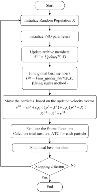
Figure 1: Finding the best local guide using Sigma method Figure 2, depicts the flowchart of the proposed MOPSO. Function Update, updates the archive members by removing

the dominated members and keeping the non-dominated ones. Selecting the global best partcile (pig,t) for each partcile is done in Find_global_best using Sigma method. Based on dominancy concept, the local best particle (pit) for each particle is updated by the function Find_local_best in each iteration. pit is like a memory for the particle i and keeps the non-dominated (best) position of the particle i. If neither pit nor particle i dominates each other, local best particle can be either of them, which is usually selected by random.

) ( ) ( , 2 2 1 1 1 t t t gt t t _{wv cr p X c r p X} v+ = + × − + − 1 1 + + ₌ t₊ t t _{X v} X

Figure 2: Flowchart of the proposed Multi-objective Particle Swarm Optimization (MOPSO)

B. Strength Pareto Evolutionary Algorithm (SPEA)

Dominance is an important concept in multi-objective optimization. In case of a two-objective minimization problem (f1 and f2), f1 is said to dominate f2 if no component of f1 is greater than the corresponding component of f2 and at least one component is smaller. Accordingly, we can say that a solution x1 dominates x2, if f(x1) dominates f(x2). A set of optimal solutions in the decision space which are not dominated by other solutions, is called Pareto set and its image on the objective space is called Pareto-front [6]. Figure 3 illustrates the main concept of Pareto optimality for sample two-objective min-min and min-max problems.

Figure 3: Main concept of Pareto optimality

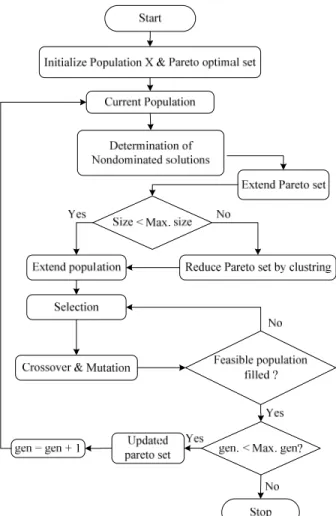
SPEA uses a mixture of established techniques and new techniques in order to find multiple Pareto optimal solutions [15]. In SPEA, first of all an initial random population is generated and an empty external Pareto optimal set is created. Second, the external Pareto set is updated by adding new non-dominated solutions and removing the non-dominated ones. If the number of individuals in the extended Pareto set exceeds the defined maximum size, the size is reduced by clustering. Clustering methods are incorporated to reduce the Pareto set. However the goal is not only to prune a given set but rather to generate a representative subset which maintains the characteristics of the original set. Hierarchical clustering method is used in this paper [15]. Then after, the fitness values of all population and external Pareto set members are calculated. The fitness of the external Pareto set members which is called Strength is the number of dominated individuals divided by the number of populations plus one. It can be seen that strength of each Pareto member is proportional to the number of individuals covered by it. The fitness of population members is defined as the sum of the strengths of all external Pareto solutions by which it is covered plus one. Figures 4.(a) and 4.(b) show the values of strengths and fitness’s for two-objective min-min and min-max optimization cases, respectively.

Figure 4: Fitness calculation for two sample scenarios

Mating pool is created based on a selection algorithm from the combination of population and external set individuals. Two random individuals are selected and the better one in terms of its fitness value is copied to the mating pool. Crossover and mutation operators are applied to the mating pool and the population for the next iteration is generated. Figure 5 shows the flowchart of the proposed SPEA.

Figure 5: Flowchart of Strength Pareto Evolutionary Algorithm (SPEA)

IV. SIMULATION RESULTS

To validate the efficiency of the proposed algorithm, it has been examined on IEEE-14 bust system. The parameters used for the system are given in [2]. The life period of VAr devices (Dy) and the interest rate (ir) are assumed to be 10 years and 0.04, respectively.

Considering the upper and lower limit of the capacity of the VAr devices and also type of each device, the structure of the population is defined as figure 6. Each individual (Xi) which is considered to be a solution for the problem consists of two parts including the allocation data of slow and fast VAr devices. The value of each cell is the capacity of the VAr device which is scheduled to be installed. By this arrangement candidate buses for slow and fast VAR resources can be determined independently. The capacities of slow and fast devices are assumed discrete numbers between 0 and 0.3 which the step size is 0.02. Population size is considered as 40.

One point crossover is used and the probabilities of crossover and mutation operators are assumed 0.8 and 0.05, respectively. Proper parameter initialization leads to better convergence and variety in optimal Pareto front solutions.

Figure 6: Structure of the population

Before VAr expansion, the amount of ATC and total system costs were 0.489 and 655.1*104$, respectively. High total cost is due to the load shedding which is carried out instead of VAr expansion to mitigate voltage collapse.

Table 1 shows the installation pattern of SVC and SC devices for some of the optimal Pareto solutions. The number inside () indicates the capacity of the installed device in the candidate bus. For example 9(0.02) means that a 0.02pu VAr device is installed at bus number 9. The value of ATC is in per unit and indicates the amount of ATC from bus 2 to bus 12 for all installation patterns. Total cost is in 104$ and includes installation and operations costs.

As shown in table 1, when the value of ATC increases, the total cost also increases. Here, the main objective is to minimize total cost and maximize ATC. To ease the decision making process, a set of optimal solutions rather than only one solution is presented. Figure 7 illustrates the Pareto optimal front after 300 iterations obtained by MOPSO and SPEA methods. It can be seen that SPEA results in better Pareto front compare to MOPSO.

TABLEI

INSTALLATION PATTERN OF PARETO OPTIMAL SOLUTIONS

SVC SC ATC Total Cost

12(0.24),13(0.1) 11(0.08) 0.711 91.13 12(0.24),13(0.16) 11(0.1),14(0.18) 0.765 103.3 12(0.26),14(0.23) 11(0.18),13(0.2) 0.789 109.3 12(0.28),13(0.21) 11(0.2),13(0.22) 0.803 111.9 12(0.28),14(0.23) 13(0.26),14(0.28) 0.895 132.1 12(0.3),14(0.26) 11(0.28),14(0.3) 0.969 147.8 0.4 0.6 0.8 1 1.2 1.4 1.6 80 100 120 140 160 180 200 220 240 260 Total Cost (10 Thousnads $)

AT

C (pu) SPEAMOPSO

Figure 7: Pareto optimal solutions after 300 iterations

V. CONCLUSION

In this paper, VAr expansion problem is treated as a min-max multi-objective optimization problem with two objective functions: (1) total cost including investment and operation costs, (2) amount of ATC. Strength Pareto Evolutionary Algorithm (SPEA) and Multi Objective Particle Swarm Optimization (MOPSO) are used to solve the problem. Solutions of the optimization problem simultaneously enhance the amount of ATC, reduce the installation and operation costs, and mitigate any system security constraints violation under normal and contingency states.

The proposed approach has been successfully tested on IEEE 14 bus test system. The results indicate that the proposed evolutionary approaches are efficient for solving the multi objective VAr expansion problem where multiple Pareto optimal solutions can be found in one simulation run.

As future work, developing some Fuzzy rules to find the best compromised solution is suggested.

REFERENCES

[1] Wenjuan Zhang, Fangxing Li and Leon M.Tolbert, “Review of Reactive Power Planning: Objectives, Constraints, and Algorithms”, IEEE Trans. Power Syst., Vol.22, No.4, Nov. 2007, pp. 2177-2186

[2] Mehdi Eghbal, Naoto Yorino, E.E.El-Araby and Yoshifumi Zoka, “Multi Load Level Reactive Power Planning Considering Slow and Fast VAR Devices by means of Particle Swarm Optimization”, Proc. of IET Transaction on Generation, Transmission and Distribution, Vol. 2, Issue 5, September 2008, pp.743-751

[3] North American Electric Reliability Council (NERC) report, “Available Transfer Capability Definitions and Determination”, June 1996 [4] Wang Feng and G.B.shrestha, “Allocation of TCSC Devices to Optimize

Total Transmission Capacity in a Competitive Power Market”, in Proc. Of Power Engineering Society Winter Meeting, 2001. IEEE, Vol.2, pp.587-593.

[5] W.ongsakul and P.Jirapong, “Optimal Allocation of FACTS devices to enhance total transfer capability using evolutionary programming”, in Proc. Of 2005 IEEE international Symposium on Circuits and Systems, Vol.5, pp.4175-4178

[6] Kalyanmoy Deb, Multi-objective optimization using Evolutionary Algorithms, John Wiley, 2001

[7] M.A. Abido, “Multi-objective evolutionary algorithms for electric power dispatch problem”, IEEE Trans. On Evolutionary Computation, Vol.10, No.3, June 2006, pp.315-329

[8] M.A. Abido, “Multi-objective Optimal Power Flow using Strength Pareto Evolutionary Algorithm”, Proc. Of the 39th International Universities Power Engineering Conference (UPEC),Vol.1,6-8 Sept. 2004 pp. 457-461

[9] Lin Zhang, Bin Ye, Quanyuan Jiang and Yijia Cao, “Application of multi objective evolutionary programming in coordinated design of FACTS controllers for transient stability improvement”, in Proc. Of Power Systems Conference and Exposition, 2006. PSCE '06. 2006, pp.2085-2089

[10] Hiroyuki Mori and Yoshinori Yamada, “An efficient Multi-objective Meta-heuristic method for Distribution Network Expansion Planning”, Proc. of IEEE PES Power Tech Conference (CD-ROM), Lausanne, July 2007,pp.1-6.

[11] Klaus Habur, Donal O’Leary, “FACTS For cost effective and reliable transmission of electrical energy”, Available at: www.worldbank.org/html/fpd/em/transmission/facts_siemens.pdf

[12] Eckart Zitzler, Kalyanmoy Deb,Lothar Thiele, “Comparison of Multiobjective Evolutionary Optimization Algorithms: Empirical results”, Evolutionary Computation, 2000,Vol.8(2), pp.173-195

[13] J.Kennedy and R.Eberhart, “Particle swarm optimization,” in Proc. of IEEE International conference on Neural Networks, Vol. IV, Perth, Australia, 1995, pp. 1942-1948

[14] S.Mostaghim and K.Y.Teich, “Strategies for finding good local guides in multi-objective particle swarm optimization (MOPSO)” in proc. IEEE Swarm Intelligence Symposium,2003, pp.26-33

[15] E.Zitzler and L.Thiele, “An Evolutionary Algorithm for Multi-objective Optimization: the Strength Pareto Evolutionary Approach”, Swiss Federal Institute of Technology, TIK-Report, No.43, 1998