Japan Advanced Institute of Science and Technology
https://dspace.jaist.ac.jp/
Title
An agent-based approach to identification of
prediction models
Author(s)
Ma, Tieju; Nakamori, Yoshiteru
Citation
International Journal of Uncertainty, Fuzziness
and Knowledge-Based Systems, 11(4): 495-514
Issue Date
2003-08
Type
Journal Article
Text version
author
URL
http://hdl.handle.net/10119/5026
Rights
Electronic version of an article published as
International Journal of Uncertainty, Fuzziness
and Knowledge-Based Systems, 11(4), 2003,
495-514. DOI:10.1142/S021848850300220X. Copyright
World Scientific Publishing Company,
http://dx.doi.org/10.1142/S021848850300220X
Description
of Uncertainty, Fuzziness and Knowledge-Based Systems, World Scientific, vol 11.4, pp.
OF PREDICTION MODELS
TIEJU MA and YOSHITERU NAKAMORI
School of Knowledge Science, Japan Advanced Institute of Science and Technology 1-1 Asahidai, Tatsunokuchi, Ishikawa 923-1292, Japan
This paper presents an agent-based approach to identification of prediction models in two-dimensional data spaces. A number of agents are sent to the two-dimensional data space that people want to investigate. At the micro-level, every agent tries to build a local linear model by competing with others, and then at the macro-level all surviving agents build the global model by cooperating with each other. And a genetic algorithm is introduced for improving the global model built by the agents. Two examples that apply this approach are given. The advantages of this approach are it does not need people to give a certain formula in advance; and most of time, it can give more precise prediction models than those given by traditional methods.
Keywords : agent, local linear model, global model, data space.
1. Introduction
During the 1980s and 1990s, many disciplines converged into an interdisciplinary research field, i.e. research on complex adaptive systems. A belief underlying this complex adaptive systems research is that macro-level complexity of the system may spontaneously be derived from the interactions at the micro-level and that this fundamental mechanism should be common among different systems in different fields. As a consequence, agent-based modeling has been applied to many fields in the last decade. Such works can be seen in Gerara Ballot and Erol Taymaz (1999)1,
Miller John H. (1998)2, Jim Doran (1994)3, Ostrom Thomas M. (1988)4, Beuu Roy
(1998)5, Derek W. Bunn and Fernando S. Oliveira (2001)6, and so on.
Prediction can be viewed as the construction and use of a model to assess the class of an unlabeled sample, or to assess the value or value ranges of an attribute that a given sample is likely to have7. Prediction of discrete or nominal values can
Induction, Bayesian Classification, Classification by Backpropagation, Classification Based on Concepts from Association Rule Mining, and so on. And for the prediction of continuous values, it is always modeled by statistical techniques of regression. We intend to apply agent technology to identify prediction models in a bottom-up way. As a first step of this plan, the approach presented in this paper deals with the prediction of continuous values with two dimensions.
Modeling by statistical techniques of regression is something like a top-down way. People first observe the distribution of all the data, form a whole structure of the data space in their minds, then select a certain function to fit the data by experience and specific knowledge. For example, for the data distribution in Fig. 1 a, people will select linear model y = ax + b; for the data distribution in Fig. 1 b, people may select exponential function y = ax+ b; and for the data distribution in Fig. 1 c, people may select sine or cosine function y = a sin x + b or y = a cos x + b. But how about the data distribution in Fig. 2 or more complex distributions? It is very difficult or impossible to find a function to fit the whole data distribution by using statistical techniques of regression in a top-down way. Certainly we can divide all the data in Fig. 2 into several parts, and for every part we find a function to fit it. But when we deal with high-dimensional data, for example 6-dimensional data, how can we know where we should separate the data. This paper puts forward the idea that we can find the whole structure of data space by agent technology in a bottom-up way, and the approach presented in this paper is elicited by this basic idea.
Fig. 1. Cases which are easy for modeling.
A simple description of the approach presented in this paper is as follows. A number of agents are sent to the two-dimensional data space that we want to investi-gate. At the micro-level, individual agents use linear regressions to build local linear models in their territories; at the same time, they try to expand their territories by finding new data objects in their visions. Correlation coefficients are used as rules to decide whether agents succeed in expanding their territory or not. During the process of expanding their territories, there is survival competition among agents. Then at the macro level, the local linear models built by those surviving agents are integrated into a global model by introducing membership functions and applying a genetic algorithm.
Fig. 2. A case which are difficult for modeling.
are p1, p2 and p3. Considering the argument that ”modeling is an art”8, Y.
Nakamori point out that, without using educated and informed intuition, it is difficult to obtain a convincing model that can be used in an actual situation 9.
According with this argument, it is necessary to join logic and intuition together and avoid combinatorial explosion for setting the three parameters. The second numerical example in section 5 shows human’s informed intuition can play an im-portant role during the process of modeling.
2. Standardizing Data Set
Before investigating a data set, it is necessary to standardize it to simplify the later work. Suppose that the raw data set is O = {(x0
1, y01), (x02, y20),· · · (x0N, y0N)}. We
call oi(x0i, yi0) ∈ O a data object of data set O. It can be standardized in both
X-dimension and Y -dimension with Eq. (1) and Eq. (2) xi= (x0 i− x0min)× SpaceXSize x0 max− x0min , (1) yi= (y0
i− y0min)× SpaceY Size
y0
max− ymin0
. (2)
Here x0
i indicates the value of X-dimension of object oi, xi indicates the
stan-dardized x0
i, x0max indicates the maximum value of O in X-dimension, x0min
indi-cates the minimum value of O in X-dimension, SpaceXSize indiindi-cates the size of X-dimension of the space in which we will put all data objects; y0i indicates the value of Y -dimension of object oi, yi indicates the standardized yi0, ymax0 indicates
the maximum value of O in Y -dimension, ymin0 indicates the minimum value of O in Y -dimension, and SpaceY Size indicates the size of Y -dimension of the space. The setting of SpaceXSize and SpaceY Size depends on the accuracy requirements of the result. If the accuracy requirements are high, they should be set big, otherwise they can be set a little small. In the rest of this paper, the setting of SpaceXSize and SpaceY Size also follows this rule: they are big enough to meet the accuracy requirements when all the values are standardized into integers. As an approach it is not necessary to follow this rule; the rule is used just for simplifying the work
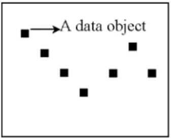
of programming. In the rest of this paper we also set SpaceXSize = SpaceY Size, which is also for simplifying the work of programming. After standardized the data set, we can build a data space and put all the data objects into it. As shown in Fig. 3, points indicate the data objects.
Fig. 3. Data space.
3. Agents and Building Local Linear Model 3.1. Initializing Agents
From a programming perspective, agent technology is a further development of the object-oriented technology. There are many definitions of agent. In this paper, an agent is simply defined as a programmed unit.
If totally there are N data objects, then after building the data space, N agents are sent into it, and each agent mounts on a data object. Each agent is initialized like the following:
Level: level = 1, Vision: p1,
Strength: s = 0.
Fig. 4. Vision of an agent.
after competing with each other, some agents will evolve into high levels and some agents will die. Every agent has a vision, which means its ability to observe the environment. As shown in Fig. 4, in its field of vision (indicated by the circle), the agent mounting on data object o2can see another two data objects, o1and o3. The
p1 can be seen as a design parameter, and the setting of it need human’s informed
intuition. An agent’s strength indicates its power of building a global structure of the data space by cooperating with other agents. For an agent of level 1, its strength is 0 because it does not participate in the construction of the global structure that is done by higher level agents.
Besides the above properties, the agents in our approach also have built-in knowl-edge and instinct. Every agent knows the regression method, and it expands its territory by instinct.
3.2. Building Local Linear Model
After initialization, every agent tries to build a local linear model according to the following steps:
• Step 1: The agent counts the number of objects in its vision. If the number is smaller than 3, this agent dies; otherwise it goes to step 2.
• Step 2: The agent does linear regression analysis of all the data objects in its vision. If the correlation coefficient r ≥ p2, it goes to step 4; otherwise it go
to step 3. Here p2 is another design parameter.
• Step 3: The agent decreases its vision by 1, that means pt+11 = pt1− 1 (here t
means time). If pt+11 = 0 it dies; otherwise it goes to step 1.
• Step 4: The agent builds a local linear model and evolves into an agent with level 2.
This progress also can be shown as in Fig. 5. 3.3. Expanding Territory
Those agents that evolve into level-2 agents try to expand their territories. Here an agent’s territory means the subspace that includes all the data objects used by the agent to build its local linear model. As shown in Fig. 6, if agent A builds a local linear model based on data objects o1, o2, o3, o4 and o5, then its territory is the
area which includes these five data objects. Although an agent’s territory is shown as an ellipse in Fig. 6, it has no special shape. In fact it is a set of the data objects that are used by the agent to build its local linear model. Another thing worthy of attention is that a data object can be in several agents’ territories. As shown in Fig. 6, the data objects o4 and o5belong to both agent A’s territory and agent B’s
territory. Also an agent can move in its territory. For example, the agent A in Fig. 6 can move from the position of data object o1 to the positions of data object o2,
Fig. 5. The process of building local linear models.
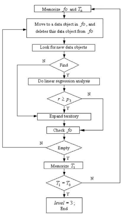
An agent expands its territory according to the following steps:
• Step 1: The agent finds all frontier data objects, and memorizes them in a list f o. The agent also memorizes its current territory as T0.
• Step 2: The agent moves to the location of a frontier data object in its terri-tory.
• Step 3: The agent looks for new data objects in its vision. If it finds new data objects, it goes to step 4; otherwise it goes to step 5.
• Step 4: The agent does linear regression analysis with the data objects in T0
and these new data objects. If the correlation coefficient r ≥ p3, the agent
succeeds in expanding its territory, that is to say these new data objects are included in this agent’s territory; otherwise it fails to expand its territory. • Step 5: If there are another frontier data objects in list fo that the agent
has not visited, it moves to one of them and goes to step 3. If the agent has visited all the data objects in the list f o, it memorizes its current territory as T1 and then goes to step 6.
• Step 6: If T1 = T0, the agent stops expanding its territory and evolves into
level 3; otherwise it goes to step 1. This progress can be shown as in Fig. 7.
An agent finds the frontier objects of its territory in the following way:
If the number of all data objects in its territory is M and the distance between two data objects oi(xi, yi) and oj(xj, yj) is dij =
p
(xi− xj)2+ (yi− yj)2, then the
agent gets the distance matrix D:
D = d11 d12 · · · d1M d21 d22 · · · d2M .. . ... ... ... dM 1 dM 2 · · · dM M . (3)
The agent ransacks D and finds the biggest distance values. The data objects that form these biggest values are marked as frontier data objects by the agent. For example if d23is one of the biggest distance values, then data objects o2 and o3 are
marked as frontier objects.
Along with the progress of agents’ expanding their territories, there is compe-tition among agents for survival in the data space. After an agent has expanded its territory (at the end of step 5), it checks whether there are other agents whose territories are covered by its territory. If there are, it eats those agents, i.e. those agents are removed from the data space. As shown in Fig. 8, agent A eats agent B. Those agents that expand their territories more efficiently and more effectively will have more chance to survive. In this sense, expanding its territory can be seen as a manifestation of an agents’ instinct for survival.
Fig. 8. Agent A eats agent B.
4. Forming Global Model
When there are only level-3 agents left in the data space, they begin to build the global model that is formed by integrating local linear models. Here the integration is done by introducing membership function (Fuzzy model). Fig. 9 shows a simple example with two local linear models or two rules10. For the first local linear model
(or rule: x is small), the membership function is µ1(x); for the second local linear
model (or rule: x is large), the membership function is µ2(x). For a certain x value
x = x∗, if µ1(x∗) = c, µ2(x∗) = d, the output of the first local linear model is yc,
and the output of the second is yd, then the estimation of y is:
y∗ =c· yc+ d· yd
c + d . (4)
If there are H level-3 agents left in the data space, the set of these agents is: A ={A1, A2,· · · , AH}. (5)
For every agent Ai ∈ A(i = 1, 2, · · · , H), it holds a local linear model yi =
fi(x) = aix + bi. Suppose that wi(x) is x’s membership value for Ai, then the
global model is:
y = H P i=1 wi(x)fi(x) H P i=1 wi(x) . (6)
In Eq. (6), we can see every surviving agent contributes to the final global model with different weight. Corresponding to the ’competition’ that we have used when describing the process of agents expanding their territories, we’d like to say agents cooperate with each other to build the global model.
Now the problem is how to get wi(x)(i = 1, 2,· · · , H). Three factors are
consid-ered. The first is agent Ai’s strength, the second is the correlation coefficient of the
local linear model built by agent Ai, and the third is the distance between x and
agent Ai.
As discussed in Section 3, an agent’s strength indicates its power to build global model. We define an agent’s strength in the following way. If there are N data objects in the data space and Mi data objects in agent Ai’s territory, then Ai’s
strength is:
si=
Mi
N . (7)
To define the distance between x and agent Ai, we first define agent Ai’s center
in the X-dimension. Suppose for the data object oj(j = 1, 2,· · · , Mi), its value in
the X-dimension is xj, then agent Ai’s center in the X-dimension is:
Cix= Mi P j=1 xj Mi . (8)
The distance between x and agent Ai is defined as:
di(x) =|x − Cix|. (9)
And wi is defined as:
wi(x) = ki
siri
edi(x). (10)
Here ri is the correlation coefficient of the local linear model built by agent Ai, and
ki is a design parameter that will be used to minimize the mean squared residual
of the global model. Suppose the set of ki for A in Eq. (5) is:
K ={k1, k2,· · · , kH}. (11)
It is possible that the set K has too many elements (parameters) in it, for example, if there are 1000 agents surviving, then the number of elements (parameters) in set K will be 1000. It will be difficult to optimize so many parameters with traditional optimization methods. So instead of aiming at optimization, the strategy here is to improve K with certain resources that users can afford. The following genetic algorithm will be used to identify K.
• Step 1: Randomly initialize a set that includes L K, as shown in Eq. (12): KSt={K1t,· · · , KLt}(t = 0). (12) Here the superscript t denotes time step.
• Step 2: For each Kt
j(j = 1,· · · , L), according to Eq. (6), Eq. (7), Eq. (8),
Eq. (9) and Eq. (10), calculate the residual sum of squares δj of the global
model and get a set:
Rt={δ1t,· · · , δtL}. (13)
Suppose δmaxis the maximum value in Rt, then for every Kjt(j = 1, 2,· · · , L)
in KSt, its possibility of being the genome of the next generation K is:
P (Kjt) = δtmax− δjt L P l=1 (δt max− δlt) . (14)
• Step 3: t = t+1, generate the next generation KStby crossover and mutation.
If t < V , go to step 2; otherwise go to step 4. • Step 4: If δt
q is the minimum value in Rt, then the Kqt in KSt is selected to
build the global model. • Step 5: End.
In the above, for generating enough genomes and better results, we recommend that L be not smaller than 10 and V be not smaller than 500. Introducing the genetic algorithm here does not mean people have to use it to identify K. People can use other optimization methods according to actual situations.
The global model given by Eq. (6) is based on the standardized data set. Cor-responding to Eq. (1) and Eq. (2), for getting the global model for the raw data set, linear conversions should be done according to Eq. (15) and Eq. (16) :
x0= x 0 max− x0min SpaceXSizex + x 0 min, (15) y0 = y0max− ymin0 SpaceY Sizey + y 0 min. (16)
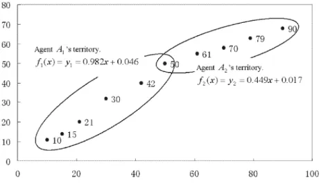
Now we give a simple example to show how the level-3 agents build the global model. As shown in Fig. 10, there are 10 data objects in the data space. At the beginning, 10 agents are sent into the space. After the competition of survival,there are only two level-3 agents left in the data space: agent A1and agent A2. The
num-ber beside every data object indicates the data object’s value in the X-dimension. There are 6 data objects in agent A1’s territory and 5 data objects in agent A2’s
territory. According to Eq. (7), The strengths of these two agents are:
Fig. 10. A simple example for building global model.
s1= 6/10 = 0.6,
According to Eq. (8), the centers in the X-dimension of these two agents are: C1x= (10 + 15 + 21 + 30 + 42 + 50)/6 = 28,
C2x= (50 + 61 + 70 + 79 + 90)/5 = 70.
Then, according to Eq. (9), the distances between x and these two agents are: d1=|x − C1x| = |x − 28|,
d2=|x − C2x| = |x − 70|.
Suppose r1= 0.9, r2= 0.96, k1= 0.2, and k2= 0.3, according to Eq. (10), we can
get: w1(x) = k1 s1r1 ed1(x) = 0.108e −|x−28|, w2(x) = k2 s2r2 ed2(x) = 0.144e −|x−70|.
Then, according to Eq. (6), we can get the global model of the data space:
y = 2 P i=1 wi(x)fi(x) 2 P i=1 wi(x) =3e|x−70|(0.982x + 0.046) + 4e|x−28|(0.449x + 0.017) 3e|x−70|+ 4e|x−28| .
This example just focuses on how to integrate local linear models to get the global model. It is just an assumption that there are two level-3 agents left in the data space after competition.
In real applications, it is possible there are hundreds of level-3 agents after competition. We can not know the real number of level-3 agents until the multi-agent system gives us the result. To a great extent, the number of level-3 multi-agents depends on how we set the design parameters p1, p2and p3. For setting these three
design parameters, it is necessary to join logic and intuition together and avoid combinatorial explosion. Generally, the bigger the p1 is set, the less agents will
survive, because with bigger visions (see Fig. 4), the agents have more chance to eat each other; the bigger the p2 is set, the less agents can survive, because with a
bigger p2there will be less agents which can evolve into level-2 agents (see Fig. 5);
and the bigger the p3is set, the more agents can survive, because with a bigger p3
it will be more difficult for agents to expand their territories, and then the agents have smaller chance to eat each other (see Fig. 7). In the next section, we will give two examples that apply the approach presented in this paper and show how informed intuition affect modeling.
5. Two Numerical Examples
In this section, we will use the approach presented in this paper to deal with two real two-dimensional numerical cases.
Table 1. Time of fall in seconds vs. radius of falling sphere of paraffin.
Raw dataset Standardized dataset.
x0 y0 x y 0.00415 1.5 200 0 0.00372 3.2 176 3 0.00369 2.5 175 2 0.00354 3.4 167 3 0.00343 3.75 161 4 . . . . . . . . . . . . 0.000527 106 1 172 0.0005 123.2 0 200 x0 max= 0.00415 y0max= 123.2 x0 min= 0.0005 y0min= 1.5
5.1. Example 1
The data set in Table 1 is time of fall in seconds vs. radius of falling sphere of paraffin in cm. It comes from UCI (University of California, Irvine) machine learning repository11. We set SpaceXSize = SpaceY Size = 200. The raw data set
is standardized according to Eq. (1) and Eq. (2). If we look every oi(xi, yi) as a
data object, there are 68 data objects in the data space. As shown in Fig. 11 1, a point indicates a data object.
We send 68 agents into this data space and set p1 = 40, p2 = 0.7, p3 = 0.99,
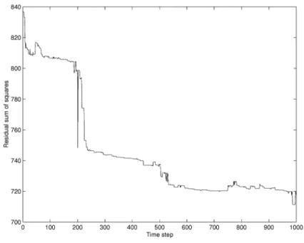
L = 40, and V = 1000. For the genetic algorithm, the crossover rate is set to be 0.7 and the mutation rate is set to be 0.02 for identifying the K in Eq. (11). Fig. 11 2 shows the local linear models built by agents at the beginning. After agents expand their territories and compete to survive, only 12 agents survive. Fig. 11 3 shows the local linear models built by these 12 agents. In Fig. 11 2 and Fig. 11 3, one circle means an agent, but that does not mean an agent is a circle. One circle is just a symbol of an agent. Fig. 11 4 shows the global model built by integrating those local linear models built by surviving agents. Fig. 12 shows the residual sum of squares ( 68 P i=1 e2 i = 68 P i=1 (y0
i− ˆyi0)2) at each step of the genetic algorithm. We can see
that although the genetic algorithm can’t ensure to find the optimizing solution, it can improve the solution little by little.
Fig. 12. Residual sum of squares at each step of the genetic algorithm (Example 1).
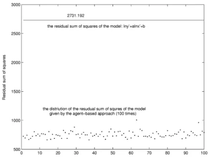
Fig. 13. Distribution of the residual sum of squares (Example 1).
data set. After using regression analysis, the model will be y0= 5.012× 10−5x0−1.9,
and the residual sum of squares will be 2731.192. The agent-based approach intro-duced in this paper is a kind of soft computing method. The residual sum of squares is not absolutely the same at every time when we run the programming. We ran the programming of the agent-based approach for 100 times, and after doing linear conversions according to Eq. (15) and Eq. (16), the average value of the residual sum of squares of the model in Fig. 11 4 is 769.116. Fig. 13 shows the distribution of the residual sum of squares of the 100 times. Compared to the model given by the traditional approach, the global model given by the agents fits the data objects better.
5.2. Example 2
The data set in Table 2 is the personal income and gross saving of America from 1929 to 2000 in billions of dollars12. We also set SpaceXSize = SpaceY Size = 200. There are totally 72 data objects in the data space. The settings of the parameters (p1, p2, p3, L and V ) are just the same as in the example 1. And for the genetic
algorithm, the crossover rate is set to be 0.7 and the mutation rate is set to be 0.02. In a traditional way, people will build a model like y0 = ax0+ b for this raw data
set. After using regression analysis, the model will be y0 = 0.205x0+ 38.864, and the residual sum of squares will be 945182.863. We also ran the programming of the agent-based approach for 100 times, and after doing linear conversions according
Table 2. Personal income and gross saving of America.
Raw dataset Standardized dataset
x0 y0 x y 85.3 19.2 1 2 76.5 14.9 1.0 1.0 . . . . . . . . . . . . 8319.20 1785.70 200 200 x0 max= 0.00415 y0max= 123.2 x0 min= 0.0005 y0min= 1.5
to Eq. (15) and Eq. (16), the average value of the residual sum of squares of the model in Fig. 14 2 is 12089.936. Fig. 15 shows the residual sum of squares at each step of the genetic algorithm. Fig. 16 shows the distribution of the residual sum of squares of the 100 times.
Fig. 14. The second example.
In this example, many people may prefer to select the traditional way to build a simple linear model for the data, because the correlation coefficient r is about 0.971, very close to 1. If we set the agent’s vision to be large enough (cover all the data space), the model given by the agent-based approach is just the same as the linear model obtained by using regression, as shown in Fig. 17. In this case, just one agent survives. So we can see human’s informed intuition can play an important role during the process of modeling.
Neural Networks have been widely used in economic forecasting. Now we com-pare the performance of the agent-based approach with that of a neural network by using Root-Mean-Square Error (RM SE). In Eq. 17, the Nt is the size of the
1991-Fig. 15. Residual sum of squares at each step of the genetic algorithm (Example 2).
Fig. 17. The same as the model yielded by linear regression.
2000) are used as testing data, while the 62 data records from 1929 to 1990 are used as training data. The smaller the RM SE, the better the performance of the model. The neural network we have used is a backpropagation network which has been programmed into the software Neunet13. With 3 nodes, we trained the neural
network for 1× 10⁵ times in each forecasting.
RM SE = v u u t 1 Nt Nt X i=1 ( ˆy0 i− yi0)2. (17)
In Fig. 18, the Nt is set from 1 to 20. We can see that the performance of
the agent-based approach is always better than that of the neural network except when Nt = 17. Of course, the comparison doesn’t prove that the performance of
the agent-based approach is better than Neural Networks at any occasion. 6. Conclusion and Future Work
This paper presented an agent-based approach to identify prediction models in two-dimensional data spaces. The advantage of this approach is it builds prediction models in a bottom-up way by competition and cooperation among agents; that is to say, it does not need people to give a certain formula in advance (which is very difficult in most of time) because the agents will find the right formula. Although it has not been proven that the models yielded by this approach always are better than those yielded by other approaches, this approach shows and proves the idea that agents can produce the global model by cooperation and competition with some built-in knowledge and simple rules. The models built by this approach are something like emergences. This idea is different from the one that says some software, such as Microsoft Excel, can give models according to input data. In fact, these softwares just do some calculating work, not build models; the models are built by humans. This idea is also a little different from that of the neural network which also does not need people to give a certain formula in advance. The basic elements of neural network are nerve cells which have no intelligence themselves. The agents in this paper are equipped with some knowledge and intelligence.
Now we just use this approach to deal with two-dimensional numerical data. In the real world, most of data are multi-dimensional, both numerical and categorical. For multi-dimensional data, a very difficult problem is to select variables. That is to say, in a subspace, some variables are irrelevant to the problem we are investigating; we would need to identify those variables that are relevant to the problem for getting better prediction result. Y. Nakamori and M. Ryoke have described this problem in detail and have succeed in developing an interactive approach in which human knowledge or intuition can play an important role9. For categorical data,
the problem is how to define similarity. Based on the basic thinking of this paper, we plan to develop an agent-based approach to deal with multi-dimensional data, both numerical and categorical.
Acknowledgements
We appreciate the help of Professor Robert B. DiGiovanni, a Visiting Professor of Technical Communication, Japan Advanced Institute of Science and Technology in reading the manuscript.
References
1. G. Ballot and E. Taymaz, “Technology change, learning and macro-economic coordi-nation: An evolutionary model”, Journal of Artificial Societies and Social Simulation, vol. 2, No. 2, 1999.
2. M. John, “Active Nonlinear Tests (ANTs) of Complex Simulations Models”, Manage-ment Science, 44(6), June, 1998, pp. 820-830
3. J. Doran, M. Palmer, N. Gilbert, and P. Mellars, “The EOS project: modeling Up-per Palaeolithic social change”, in Simulating Societies, eds. N. Gilbert and J. Doran (London: UCL Press, 1994) pp.195-222.
4. O. Thomas, “Computer Simulation: The Third Symbol System”, Journal of Experi-mental Social Psychology, 24(5), September, 1998, pp. 381-392.
5. B. Roy, “Using Agents to Make and Manage markets Across a Supply Web: Replacing Central, Global Optimization with a Distributed, Self-Organizing Market Approach”, Complexity, 3(4): pp.31-35, 1998.
6. W. Bunn Derek and S. Oliveira Fernando, “Agent-Based Simulation–An Application to the New Electricity Trading Arrangements of England and Wales”, IEEE Transition on Evolutionary Computation, vol. 5. No. 5. October 2001.
7. J. Han and K. Micheline,Data Mining — Concepts and Techniques, (Morgan Kaufmann Publishers, 2000).
8. G. Majone, ”The craft of applied systems analysis”, Rethinking the Process of Opera-tional Research and Systems Analysis, R. Tomlinson and I. Kiss, Eds. Oxford: Pergamon Press, 1984, pp. 143-157.
9. Y. Nakamori and M.Ryoke, “Identification of Fuzzy Prediction Models Through Hy-perellipsoidal Clustering”, IEEE Transaction on Systems, Man, and Cybernetics, vol. 24, No. 8, August 1994.
10. T. Takagi and M. Sugeno, “Fuzzy identification of Systems and its applications to mod-eling and control”, IEEE Transaction on Systems, Man, and Cybernetics, vol. SMC-15, No. 1, pp.116-132, 1985.
11. UCI machine learning repository, available at:
http://www.ics.uci.edu/∼mlearn/MLRepository.html.
12. NIPA (National Income and Product Accounts) Data, available
at:http://www.bea.doc.gov/bea/dn/nipaweb/Index.asp. 13. Available at: http://www.cormactech.com/neunet/.