Bounds and an Approximation for Single Server Queues

Journal of the Operations Research Society of Japan

Vol. 26, No. 2, June 1983

BOUNDS AND AN APPROXIMATION FOR

SINGLE SERVER QUEUES

J eyaveerasingam George Shanthikumar

Syracuse University

(Received January 6,1982; Final October 27,1982)

Abstract In this note, we derive bounds for the waiting time in a single server queueing system with general independent arrival and general service times, using a regenerative process representation of this queue. We present easily computable new upper bounds for the variance and new upper and lower bounds for the second and higher moments of the waiting time. Also W(' present a simple approximation for the variance of waiting time.

Introduction

Mori [10] presented an elaborate study of bounds for the single (GI/G/l) and multiple (GI/G/m) server queueing systems with general in-dependent arrival and service times. He has derived easily computable lower and upper bounds for the mean waiting time and a lower bound for the variance of waiting time in a GI/G/l queue. Similar results for the GI/G/m queue are also given in [10]. Upper and lower bounds for the mean and variance of ,,;raiting times for special cases of GI/G/l are also given. However, no upper bound for the variance of waiting time is given for the general GI/G/l queue (see page 168 of [10]). In this note, ,.e derive an easily computable upper bound and approximations for the variance of waiting time in a GI/G/l queue.

Considerable interest has been shown in developing bounds (see [1,2,4-10,12,15,16]) and several approximations (see [14] for a review and comparison) for the GI/G/l queue. In this paper, using a regenera-tive process representation of the GI/G/l queue, we will develop easily computable upper and lowe'r bounds for the mean, variance, second, and higher moments for the waiting time. In this process we develop easily

Bounds and Approximation for GI/G/l Queues

In section 2, we discuss the GI/G/l queueing model and derive equations relating the moments of the waiting time to the moments of idle time. W,~ also present upper and lower bounds for the moments of the idle periods. Bounds of mean waiting time is briefly discussed in section 3, and bounds for variance of waiting time is presented in section 4. A recursive scheme to compute the second and higher moments of the waiting time is discussed in section 5. A simple approximation for the variance of waiting time is given in section 6. Numerical re-sults for the bounds and approximation are given in section 7.

2. The Single Server Queue

We consider a single server queueing system to which the arrivals form a renewal process: the n-th customer arrival occurs at time 'n and requires a service of length Bn. The interarrival times

An

=

'n+l - en' n':: 1 and the service times Bn' n .:: 1, are assumed to form two independent sequences of independently and identically distri-buted random variables. Define p{An.2. x}

=

A(x), P{Bn.2. x}

=

B(x), and P{Bn - An

~

Xn

.2. x}

=

X(x).

Let Wn be the waiting time of the n-th customer, Wl

=

O. Note that {Wn}'l forms a discrete time regenerative process with regeneration epoch corresponding to the customer arrivals to an empty system. Let N be the number of customers served during the first regeneration cycle formed by the busy cycle of GI/G/l. Then,

(1) W_l

=

I)

(2) Wn + Bn - An, n

=

1,2, .... ,N-1

where WN+1

=

I) w.p. 1, and I is the server idle time during the first regeneration eyc1e. Taking the (r+1)-th power of equations (1), (2), and (3), summing up and taking the expeetations on both sides we get,

where E is th,~ expectation operator. Now assuming that

p

~

E(B)/E(A) < 1 and E(lxlj) < 00, j

=

1,2, ... ,r+1, from the theory of regenerative processes (see e.8., Crane and Lemoine [3]) we can show that

120 J.G. Shanthikumar

since Wand X are independent and W D lim W. _{n n =n __ n} Now dividing the previous equation by E(N) and using the above result one has

(_l)r+l E(Ir+l) r-l . r+l-j

(4) E(Wr) = _ _ 1_ L: (r+l)E(WJ)E(X )

(r+l) E(N)E(X) _{(r+l) j=O} j E(X) r > 1,

Similarly, summing equations (1) , (2) • and (3), and taking expecta-tions on both sides, we get

(5) E(I) = -E(N)E(X).

Then, substituting (5) for E(I) in (4), we have

(6) E(Wr ) = (_l)r E(Ir+l) 1

r~l

(r-:l)E(Wj)E(Xr+l-j ). (r+l) -E(I) - (r+l)E(X) j=O J

r .:::. 1.

a result obtained by Lemoine [7] using an alternate approach. I f we have upper and lower bounds for E(Wj). j = l.2, •.• ,r-l, and

r+l r

E(I )/E(I). we can develop upper and lower bounds for E(W). That is. (6) gives a recursive relation useful in developing bounds for the r-th moment of the waiting timE! in GI/G/l queue. Next we will develop bounds for E(Ir)/E(I). r > 2.

Now define Y =

-x .,

A - B • n = 1.2 •...• N. Multiply equation

n n n n

(1) by y~, (2) by Y:. and (3) by Y~. adding them and taking expectation, we get N E{ L: W~ y~ l} - E(IY~) i=l ~ ~-where Y O ~ Yn• n 1,2 •.... Now noting that

N

E{ L: W. Y~_l}/E(N) i=l ~

and

Bounds and Approximation for GI/G/l Queues

N

E{ ~ W. yri}/E(N) i=l 1

and dividing the above equation by E(N) one obtains,

(7) where

E(IY~)

Cov(W, yr) _ _ --,-';':-E(N)

Cov(W,yr)

=

lim Cov(Wn+l'y~). n--><x>

Cov(W,yr)

20,

for I'

=

1,3,5, ... , since as Y increases, yr increases

n n

and Wn+l will not increase. Now noting that YN ~ I, from (7) we get (8) E(Ir+1)

2

E(N)E(Xr+1), I' = 1,3,5, . . . .

I t should be noted that the upper bound for E(Ir+l) derived by Lemoine [7] (equation 2.11) is better than that given by equation (8). This bound (equation 2.11 of [7]) can be derived by a procedure similar to the above except using y+

=

max(Y ,0) instead of Y and noting that

n n n

(Y )(y+/ = (y+)r+l and y+ = YN. To compute this bound given in [7],

n n n n

however, we need to know the distribution functions A(o) and B(o).

Thus, for quiek calculations with partial information of only the moments of A(o) and B(o), equation (8) may be used and it should prove to be a useful bound.

Now dividing (8) by (5), we get

(9) I'

=

1,3,5,7, ..•

A similar derivation using An instead of Y

n gives (10) E(Ar +l ) _ E(B)E(Ar )

E(A) E(B) I' ~ 1,

Equations (9) and (10) give upper bounds for E(Ir)/E(I). Next we need to develop lower bounds for these quantities. Obviously

(11)

Stronger lower bounds can be developed using the properties of positive random variables and Jensen's inequality to convex functions. It is

122 J.G. Shanthikumar

(lZ) E(I

r_{) r-l}

E(I)':' (E(I» , r

=

1,Z, ...

An alternate equation for E(Wr) can be derived from (6) by considering the ratio of E(Ir+l)/E(Ir). It is

1 (r+l)E(X) (13)

Now to use equation (13) to derive bounds for E(Wr) w-e need upper and lower bounds for E(Ir+l)/E(Ir). Lower bounds for this can be derived as follows. Let I_k+_l be the residual life of the renewal process formed by random variables with the same cumulative distribution function

Ik(o) as that of I

k. Thai: is, /x(l-Ik(y»dy

(14) Ik+l(x) _{E Ik} ( ) k .:. 0,

where we set ₁₀ I and assume that E(I

k) < 00. Then

E(I~+l)

E(Ij+l)

(15) k k.:. 0, j _{.:. 1,}

(j+l)E(I k)

Using (15) recursively for k r-l,r-Z, ... ,O, we can show that

(16) and (17) E(Ir+l) (r+l)E(Ir) Z (r+Z) (r+l) r .:. 0, r > 0.

Then, using the property that Var(I ) _r = E(I_r Z)

(18) 2 E(I r

+

Z)

- - - > E(Il") (r+l) (r+Z) Rearranging, we get (E(I »Z > 0, we get r -r >

°

Bounds and Approximation for GI/G/l Queues

(19) (r+2)

2(r+l)

Repeated use of (19) leads to

E(lr+2) E(12) (r+2) - - - - > - - - . E(lr+l) - E(l) 2r +l (20) r >

o.

r > O.

Now we need lower bounds for E(l) or E(I2)/E(I) to use (12) and (20). The following bounds can be derived from the results available in the literature, or using equation (5).

(21) ~ E(12) > E(l) > (l-p)E(A).

The above lower bound can be derived using (5) and noting that E(N) > 1 (see Kingman '[5] and Marshall [9]).

(22) ~ E(12) > E(l) > (l-p)E(A)/X(O).

The above lower bound can be derived usi.ng (5) and noting that E(N) ..:: l/X(O) (see Mori [10] and Lemoine [7]).

Using Daley's upper bound for E(W) reported by Calo and Schwartz [1], we can show that

(23)

where

c

2 is the squared coefficient of variation of interarrival times. a

Note that (23) is a better lower bound than (21). Now, using the re-sults given in Mori [10] and (23), we get

(24)

3.

Bounds on Mean Waiting Time

In this section we indicate how th'= bounds available for E(W) in the literature can be derived from equations (6), (9), (10), (21), and (23). From (6) we get, for r

=

1,

124 J. G. Shanthikumar

(25) E(W)

Now using (25) and (9), wee get a trivial lower bound E(W) > O. However, using (25) and (10) gives the lower bound

(26) _{E(W) > 2E(A) (l-p)} Var(B) E(B) 2

derived by Stoyan and Stoyan [15J and Mori [10J. Note that when the squared coefficient of variation

c~,

of the service time is such that,

2

Cb < (l-p)/p, the lower bound (26) is negative. See Table 1 for other lower bounds available in the literature. Now usine (25) and (21), we get the upper bound of Kingman [4J and Marshall [9J. Using (25) and (22), we get the upper bound of Mori [10J and Lemoine [7J. For other upper bounds, see Table 1.

TABLE 1. Upper and Lower Bounds for the Mean Waiting Time E(W).

E(W)

LOWER BOUND UPPER BOUND

E(X+2 2 _{Kingman [ 5)}

E(A) (C!i92C~)

2(1-p)E(A)

.

, Kingman (4)

2(l-p) Marshal! I'))

w

2, the unique solution, Marshall ( 9J E (A) (C

2 _{i9 2C}2_{) (l-p )C}2_E(A) a b _{a _ , na1"l} of 2(1-p) - 2 Reporte in w = J~(l-X(x»dx -w E(A) (C2i92C2)

Var (B) _ E(B) _{, Stoyan} a b Stoyan [t 5 I

& Stoyan 2{1-p)

-

,

2(1-p)E(A) 2

[ IS) Lemoine (7)

Mori [10] (l-e)(l-X(O»E(A) 2X(0) E(X++X)+ • Calo & Schwartz

(1)

[1] w_{l '} the unique positive, Calo & Schwartz

root of [1]

E(X2)-E{(X++X)-~2

Calo & Schwartz 2(1p)E(A)w -2(1-p)E(A)

.

_[1]

Bounds and Approximation for GI/G / 1 Queues

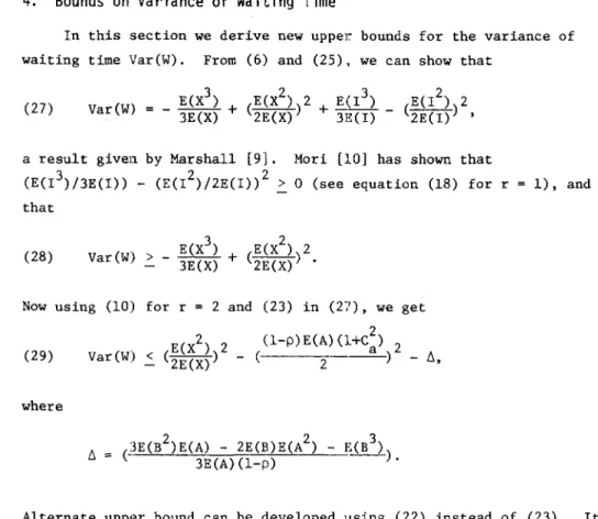
4.

Bounds on Variance of Waiting Time

In this section we derive new upper bounds for the variance of waiting time Var(W). From (6) and (25)" we can show that

(27) Var(W)

a result given by Marshal! [9]. Mori [10] has shown that (E(I3)/3E(I» - (E(I2)/2E(I»2

~

0 (see equation (18) for r that

1), and

(28)

3 2

Var(W) > _ E(X )

+

(E(X »2

3E(X) 2E(X)

Now using (10) for r

=

2 and (23) in (27), we get

(29)

where

2 (1-P)E(A)(1+C2) 2

Var(W) <

(~i~x~)2

- ( 2 a) - tJ.,

(}E(B2)E(A) _ 2E(B)E(A2) _ E(B3». 3E(A) (l-p)

Alternate upper bound can be developed using (22) instead of (23). It is

(30)

TABLE 2. Upper and Lower Bounds for Variance of \~aiting Time Var(W).

Var(I,;)

LOWER BOUND UPPER BOUND

~

E0Cl2 2 (1-p)E(A)(l+c

2_{) 2} , Mori [I'll -t, + (E(X »2 _

- 3E(X) + (2E(X) ) 2E(X) ( 2 a ) . , .

2 «1-P)E(A»2 .,. -6 + (E(X »2 _ 2E(X) 2X(O) 125 4 1

min (2"2 log(-.-)} • Kingman [5]

.,.

developed in this article

s e s l-X(s)

3E(B2)E(A) - 2E(B)E(A2) - E(B3)

126 J,G, Slumthiku/11ilT

5.

Bounds for Second and Higher Moments of Waiting Time

In this section we wHl formally present the recursive relation to

r

compute bounds for E(W ), r ~ 2. Let U

r be the upper and Lr be the lower bounds of E(Wr) for r > 1. Set U

l equal to the minimum of the upper bounds for E(W) presented in Table 1 and Ll equal to the maximum of the lower bounds for E(W) presented in Table 1. Define u

r+l equal to the minimum of the right hand side of (9) and (10). Let t1 equal the maximum of the right hand side of (22) and (23). Let tr+2 be equal to the right hand side of (12) with E(l) replaced by t

l. Then from (6) we get, for

r = 1,Z, ... ,

(31) _{uZr+l - (2r+1)E(X)} 1

r~l

(zr2+J.1)L2J,E(X2t+1-Zj)

j=O 1 r-1

_L

_{(Zr+l)U E(XZr- Zj )} Zj+1 Zj+l (Zr+l)E(X) j=O r-1 t 1

L

(zrZ+J.1)UZJ.E(Xzr+1-2j) Zr+l - (2r+l)E(X) j=O r-1 -;-:---:-7-1 L (Zr+1)L E(X2r- Zj ) (2r+1)E(X) ZJ'+l 2j+l j=O (32) r -t

Zr+2 - (Zr+2)E(X) j=O 2J 1 L (Zr:Z)U .E(X2r+Z-Zj) ZJ

_ _ _ 1 _ _

r~l

(Zr+Z)L E(XZr+1-2j) (Zr+Z)E(X) j=O Zj+1 Zj+l

_ _ _ 1 _ _

r~l

(2r+Z)U E(XZr+1-2j) (2r+2)E(X) j=O Zj+l 2j+l .

Now equations (31) and (32) can be alternatively evaluated for r

=

1,Z, ... , until the bounds for the desired moment of the queueing time is obtained.

Bounds and Approximat~Jn for GI/G/l Queues

along with (9) and (10) can be used to eompute bounds for E(Wr), r > 1.

6. Approximation for the Variance Var(W)

In this section we derive an approximation for the variance Var(W) of waiting time in the GI/G/1 queue. We know of no other approximations available for Var(W). Here we propose two approximations for Var(W), one for each of t,,,o different cases of GI/Gll. The two cases are

2 2 2 2

1 > C > C > 0 and 1 > C > C > 0, chosen purely based on numerical

- s - a - - a s

-results of

thE~se

approximations (carried out in [13]), where C2 and C2

a s

are the squarE~d coefficient of variation of the interarriva1 and service times, respectively.

The approximations are chosen following the approach similar to 3 Page's [11] and Takahashi [17]. However, weights are chosen to be Ca

4 2 2

and Cs instead of Ca and Cs because they gave better approximations. The proposed approximations are:

') 2 (i) for 1 > C- > C > O.

s - a -(33) Var(W)

where VadW(G/M)} and VadW(M/D)} are respectively the variance of time spent queueing in equivalent GI/M/1 and M/D/1 queues. The equivalent GI/M/1 queue is chosen so that its inter arrival process and server utilizations are identical to the given GI/G/1 queue. Similarly, the equivalent M/D/1 queue is chosen so that its mean arrival and service rates are identical to the given GI/G/1 queue.

Unfortunately there is no closed form solution for VadW(G/M)}. A very good approximation can be obtainE~d, however. I f E[W(B/M)] is the mean waiting time in GI/M/1 queue with mean service time E(B), it can be shown that (from the distribution function for W (G/M) [6]),

VadW(G/M) } E[W(G/M)J(E[W(G/M)]

+

2E(B» .

We have already given a very good approximation (L(PAG» for the mean

128 J. G. Shanthikumar

number in the Gr/M/1 system in [14]. Then, from equation (8) of [14] 2

with the substitution Cs

=

1, we get

E[W(G/M)] '" k, where

k pE(B) _2(1-p) {2C2 + (1_C2) _{a a exp} {-2(1- P)}} _{3p .}

Then

(34) Var{W(G/M)} '" k(k + 2E(B».

When the arrival distribution is Erlan&, a closed form for Var{W(G/M)} is available [6]. Thus we can check the approximation (33) against the exact value in the Er1ang case.

A comparison of this approximation to the exact values are given in Table 6. The exact value for Var{W(M/D)} is:

Var{W(M/D) } P(4-p)(E(B»2 ₂ 12(1-p)

Now substituting equation (34) and the above into (33), we get

(35) Var(W) 2 '" k(k+2E(B»C4 + p(4-p)(E(B» s l2(1-p)2 1 > C2 > C2 >

o.

- s - a -Similarly: (ii) for 1 > Ca > C2 > 0 we propose

- 2 s

-(36) Var(W) '" C4 Var{W(M/G)} + C3(1-C4)Var{W(D/M)},

a s a

where Var{W(M/G)} and Var(W(D/M)} are respectively the variance of time spent queueing in equival'=nt M/G/1 and D/M/1 queues. The exact value for Var{W(M/G)} depends on the third moment of the service time distri-· bution. We will approximate Var{W(M/G)} by an equivalent M/Ek/l queue so that

Bounds and Approximation for GI/G/l Queues

(37)

P(I+C2){4_p+(8_5P)C2}(E(B»2 VadW(M/G)} '" ---.::s=---;;:2---!s~ _ _ _

12(l-p)

We have already given an approximation for VadW(G/M)} by equation (34). Substituting

c

2 = 0 in (34), we get

a

where

pE(B) 2(I-p)} (38) kl

=

2(l-p) exp{- 3p .

Substituting equations (37) and (38) in (36), we get P(I+C2){4-P+(8_5P)C2}(E(B»2C4

(39) Var(W) '" s 2 s a + k

l(kl+2E(B»C;(I-C:) 12(I-p)

7. Some Numerical Comparisons

In this section, we will look at the goodness of the bounds and the approximation for the variance of waiting time in Ek/E~/l queueing sys-tems. For M/E~/l and Ek/M/I exact results are obtained and compared to the bounds (see Tables 3 and 4) and to the approximations (see Table 6). For other cases, simulation is used to obtain estimates of the variance of waiting time. These results, with the bounds are given in Table 5 and with the approximations are given in Tables 7 and 8.

We observed that the bounds are good in general only when the server utilization is higher than .6. It is also observed that the lower bound is closer to the exact result than the upper bound. How-ever, when the server utilization is lower than .6, most of the time the lower bound is negative and the upper bound is very much higher than the exact value. Of course, the negative values of the lower bound (27) should be read as zero. Thenlfore, it is strongly suggested that the bounds be used only for cases with high server utilizations.

130 J.G. Shanthikumar p+ .6 .7 .8 .9

TABLE 3. Exact:, lower and upper bounds for the variance of waiting time of an arbitrary customer in an M/E£/l queue for various values of the Er1ang parameter £ of E£ and server utilization p.

Variance of Waiting Time Var(W)

!/,-+ 1 2 LB 2.".722 -0.0122 EX 5.2:500 2.7656 UB 10.3611 7.8769 LB 8.0703 3.3500 EX 10.1111 5.3958 UB 15.1429 10.4276 LB 22.~375 11. 4375 EX 24.0000 13.0000 UB 29.6667 18.6667 LB 97.7654 53.3279 EX 99.0000 54.5625 UB 107.6296 63.1921 LB - Lower Bound (equation (28» EX - Exact

UB - Upper Bound (equation (29»

3 5 -0.6667 -1.1278 2.1111 1.6500 7.2222 6.7611 2.1073 1. 2259 4.1481 3.2667 9.1799 8.2984 8.5116 6.4375 10.0741 8.0000 15.7407 13.6667 41. 4321 32.9654 42.6667 34.2000 51. 2963 42.8296 10 -1. 4372 1.3406 6.4517 0.6328 2.6736 7.7054 5.0375 6.6000 12.2667 27.2279 28.4625 37.0921

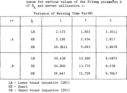
TABLE 4. Exact, lower and upper bounds for the variance of waiting time of an arbitrary customer in an E

k/M/1 queue for various values of the Er1ang parameEer k of Ek and server utilization p.

Variance of Waiting Time Var(W)

p.j. k 1 -+ LB 2.472 .6 EX 5.250 UB 10.3611 LB 22.438 .8 EX 24.000 UB 29.667 2 1.821 2.934 5.043 13.160 13.774 15.729 5 1. 3611 1.817 2.8678 8.6875 8.938 9.7067

Bounds and Approximation/aT GI/G/l Queues

TABLE 5. Simulated results, lower and upper bounds for the variance of waiting time of an arbitrary customer in an ~/ER./l queue for various values of the

p

0.8

0.6

Erlang parameters k and £ of ~ and E£ and server utilization p

=

0.6.

Variance of Waiting Time Var(W)

k+ £-+ 2 LB 0.118 2 SIM 1.248 UB 3.340 LB 0.127 5 SIM 0.517 UB 1.633

LB - Lower bound (equation (28» SIM - Simulation results UB - Upper bound (equation (29»

5 -0.529 0.472 2.693 -0.239 0.204 1.268

TABLE 6. Variance of Waiting Time in the Ek/M/l Queue

C2 EXACT APPROXIMATE a 1.0 24.000 24.000 0.5 13.774 13.795 0.2 8.938 8.950 0.1 7.541 7.548 0.0 6.250 6.252 1.0 5.250 5.250 0.5 2.934 2.962 0.2 1.817 1.838 0.1 1.491 1.505 0.0 1.190 1.193 131

132 J. G. ShanthikuTl1ll1'

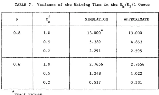
TABLE 7. Variance of the Waiting Time in the ~/E2/1 Queue

p C2 Cl SIMULATION APPROXIMATE

*

0.8 1.0 13.000 13.000

o

.~) 5.389 4.863 0.2 2.291 2.595 0.6 1.0 2.7656 2.7656 0.5 1.248 1.022 0.2 0.517 0.531

*

Exact values

TABLE 8. Variance of the Waiting Time in the ~/E5/1 Queue

p C2 SIMULATION APPROXIMATE a

*

0.8 1.0 8.000 8.000 0.5 2.489 2.419 0.2 0.679 0.816

*

0.6 1.0 1.650 1.650 0.5 0.472 0.493 0.2 0.204 0.165

*

Exact values

The proposed approximation given exact values for M/E

k/1 systems, very good approximations for ~/M/1 systems, and reasonably good

approx-Bounds and Approximation for GI/G/I Queues

Acknowledgements

The author would like to thank the referees for their helpful comments.

References

[1] Ca10, S. B. and Schwartz, S. C: An Upper Bound for the Equilibrium Mean Wait in a Stationary GI/G/1 Queue. Mathematics of Operations Research, Vol. 2 (1977), 240-243.

[2] Cox, D. R. and B1oomfie1d, P.: A Low Traffic Approximation for Queues. Journal of Applied Probability, Vol. 9 (1972), 832-840. [3] Crane, H. A. and Lemoine, A. J.: An Introduction to the Regenerative

Method jor Simulation Analysis. Springer-Ver1ag, 1977.

[4] Kingman, J. F. C.: Some Inequalities for the GI/G/1 Queue. Bio-metrika, Vol. 49 (1962), 315-324.

[5] Kingman, J. F. C.: Inequalities in the Theory of Queues. Journal of Royal Statistical Society, Series B, Vol. 32 (1970), 102-110. [6] K1einrock, L.: Queueing Systems, Volume 1. Wi1ey Intersciences,

1976.

[7] Lemoine, A. J.: On Random Walks and Stable GI/G/1 Queues. Mathematies of Operations Research, Vol. 1 (1976), 159-164.

[8J Marchal, W. G.: Simple Bounds on the Idle Time and Busy Period Distributions in the GI/G/1 Queue. Paper presented at the 1979 ORSA/TIMS Conference, Milwaukee (1979).

[9] Marshall, K. T: Some Inequalities in Queueing. Operations Research,

Vol. 16 (1967), 651-658.

[10] Mori, M.: Some Bounds for Queues. Journal of the Operations Research Society of Japan, Vol. 18 (1975), 152-181.

[11] Page, E. S.: Queueing Theory in OR. Crane Russak & Company, Inc., New York (1972).

[12] Ross, S.M.: Bounds on the Delay Distribution in GI/G/1 Queue.

Journal of Applied Probability, Vel. 11 (1974), 417-421.

[13] Shanthikumar, J. G.: Approximate (iueueing Models of Dynamic Job Shops, Ph.D. Thesis, Univ' ,:sity of Toronto, Toronto (1979). [14] Shanthikumar, J. G. and Buzacott, J. A.: On the Approximations to

the Single Server Queue. Internati:onal Journal of Productions Research, Vol. 18 (1980), 761-773.

134 J.G. Shanthikumar

[15] Stoyan, D.: Bounds and Approximations in Queueing Through Monotoni-city and Continuity. Operations Research, Vo1. 25 (1977), 851-863. [16] Stoyan, D. and Stoyan, H.: Bounds on the Mean Waiting Time in One-Channel Systems of Mass Service. Engineering Cybernetics, Vol. 12

(1974), 79-81.

[17] Takahashi, Y.: An Approximation Formula for the Mean Waiting Time of an M/G/c Queue. ,.journal of the Operations Research Society of Japan, Vol. 20 (1977), 150-163.

Dr. J. G. Shanthikumar: Associate Professor

Syste~s and Industrial Engineering University of Arizona

Tucson, AZ 85721 U.S.A.