Some Discussions on Power Load Prediction Based on Farmer's Method

J. Operation Research Soc. of Japan Vol. 10, Nos. 3 & 4, June 1968

SOME DISCUSSIONS ON POWER LOAD PREDICTION

BASED ON FARMER'S METHOD

MORIKI TOYAMA and KEIGO YAMADA

1. Introduction

Mitsubishi Electric Corporation (Received February 6, 1967)

The prediction of electric load takes an important part in determin-ing operation schedules of power stations and sub-stations as well as economical dispatch and load frequency control. As the techniques for this purpose they are roughly classified into two kinds. One is to esti-mate statistically by means of past load data, the other is to estiesti-mate functionaly by seeking any functional relation between electric load and measurable main factors which seem to be influential to the electric load. The Expential Smoothing Method [1] [2] and the Farmer's Method [3] which will be described in this article belong to the former and a Reg-ression Model Method [4] belongs to the latter_ They are to be employed according to the objects, for example, the former is better to predict the range from several minutes to several hours but the latter seems more appropriate to predict the peak load of the next day_

In this paper we are trying to report what we contemplate on pre-diction errors by means of experiments with actual data and on some problems which arise in its &pplication. The matters we discuss here are as follows:

(1) The relation between prediction errors and number of the cha-racteristic mode functions and other parameters which the Farmer's Method uses.

(2) Automatic detection of the load pattern change which is necessary

125

126 M. TOllama and K. Yamada

to put the Farmer's Method to practical use, especially as a part of auto· matic power f-eeding systems.

(3) Applicable method to the load series which have a certain trend in order to put this method to practical use.

2. Farmer's Method

For later discussions the abstract of the Farmer's Method will be described below.

The Farmer's Method is essentially suitable for a short time predic· tion. In such a forecasting, it is assumed that electric load doesn't have a constructive change and its pattern is almost constant. Now daily electric load is represented with x(t)(O~t~ T); where t means any daily time and T is it's final time.

In the Farmer's Method it is assumed that such electric load x(t) is represented by a linear combination of some characteristic mode functions.

The characteristic mode functions are introduced as follows: Suppose that xm(t),m=1,2, ... ,M, are M sample functions of the

stochastic process of electric load and that it is required to defie, in some sense, the characteristic modes of the process. A simple way of specifying the first mode is to seek a function (h(t), a scaling factor All 2 and a set of coefficients am , such that A11jSam (h(t) approximates, in a

1 1

least square sense, to the sample functions xm(t) over a specified time interval (0, T). The

m

th error takes the form:

( 1 )

The mean square error averaged over time and over the group is:

(2)

The function ifJ1(t) and the vector a:,.. may, without loss of generality, 1

Power Load Prediction 121 (3)

{

J:

ifJll(t)dt= 1 , M

L:

a~ =M. m=l I

The minimum conditions then take the form

(4)

On the other hand, sample correlation function R(t, T) is described with eqn (5).

(5)

From eqns (4) & (5), the following eigen function eqn (6) is introduced.

(6)

J:

R(t, T)ifJl(T)dT=).lifJl(t) O~t~ T.

Combing eqns (2) and (4) gives for the minimum mean square error

(7) E=

~H:

R(t, T)dt-).l } ,

and it is necessary to take the greatest eigen value as ).1 to minimize eqn (7).

Therefore, (h(t) is determined as the eigen function corresponding to the dominant eigen value ).1.

Furthermore the 2 nd characteristic mode function ifJ2(t) is calculated by treating em(t) as sample functions in place of xm(t), and it is proved that this function ifJ2(t) is corresponding to the 2 nd greatest eigen value ),2 of eqn (6).

128 M. TogolII4 and K. Yamada

the same manner.

Sample function takes the form: (8)

When the series in eqn (8) is terminated after K terms, the least mean square error EK is as follows:

(9)

Eqn (9) shows that it is possible to select K for the specified accuracy. Now prediction mechanism is expressed as follows, using the cha· racteristic mode functions which were described above:

K

(10) X(t)=

E

CiifJt(t). ;=1

Where X(t) is estimated load for actual load x(t)

Here it is necessary to decide the value of Ci(i=I,2,· ··,K). A simple method is to choose them such that eqn (10) is the best means square approximation to past data.

Namely that is to minimize eqn (11) when load data x(t) over a specified time interval (0, To) are given. Then it is possible to estimate the load at

et

time ahead of To with eqn (10).

(11)

In reference (3) another method is described using Volterra series expansion. But that is omitted in this paper because no experiments about it are done.

Note: On the estimation of prediction

Eqn (9) gives the evaluation of prediction error as Farmer describes. But it is apparent that this gives lower evaluation than the actual

Power Load Prediction 129 one, due to the definition itself of Ek in eqn (9).

For example, assume the following process described by eqn (12): (12)

where

x(t)= sin He(t) (O:s;t:S;2;r) e(t) is a random variable and

independent with respect to time and, average of e(t),E[e(t)]=O

variance of e(t)~ Var[e(t)] =/12•

Then, mean square prediction error is /12, but that of eqn (9) is (2)r

-1)/12_{j21t' and lower than true one ..}

Therefore, it is better that the following eqn (13) is used to make more precise evaluation about mean square prediction error.

(13) EK1= t n : R(t, t)dt -

i~.

Ai

+

If.

~:

r

rpi(t)(Pt(r:)·a(t, r:)drdtJ , ·where

a(t, r:)= R(t, r:) --x(t) x(r:)

and x(t) expresses the mean of sample functions at time

t.

Eqn (13) is introduced as follows:

Assuming that the prediction mechanism is given by eqn (14):

(14)

mean square prediction error at time .t, D(t) is defined by eqn (15).

(15)

Here, Ci( = 1,2, .. " K) which minimize the following equation:

E

D:

{XC

t) -

i~.

Clrpi(t)

r

dtJ are adopted as Cl in eqn (14) Then

130 (16)

M. T01lama tmd K. Yemade

Ci =

I:

~i(t)E[x(t)]dt

(;=1,2,·· ·,K)

According to the fact that eigenfunctions ~i(t) are orthonormal, eqn (15) is modified as follows:

K K (T

D(t)=E[x2_{(t)]-i~l Ai~iZ(t)+ 2}

£

_9S,(t)

_jo

_{9Si(r)a(t, r)dr}

-

~ ~ 9Si(t)~tCt) ~~ 9St(r)1~

9Sh)(a(1:, p»dpdr where

aCt, r)=R(t, r)-E[x(t)]E[x(r)].

Therefore, the mean square prediction error averaged over time interval (0, T) becomes as follows:

1

(T

1

[rT

EK1= T)o D (t)dt= T

)0

R(t, t)dt

Eqn (13) obtained by substituting a(t, r), which is calculated from sample ,data, in place of a(t, r) in eqn (17).

In case of eqn (12),

where

aCt, r)=q20(t-r)

{1 t=r o(t-r) = 0 t-~r and there is only one eigen value.

Power Load Prediction 131

3. Experiments Based on the Actual Date and Discussions on Them Some discussions on experimental results with the actual data are described below by means of the Farmer's Method which was described in chapter 2. We would like point out several problems which are to be considered when this method is applied.

(a) How many samples are necessary to make the characteristic mode functions? In connection to this, too much samples are not proper as Farmer points out. This is because they may be affected by the past data of different pattern. According to Farmer's report twenty samples are employed, but our experience indicates that such large samples are apt to be affected by the past data of different pattern so that the pre-diction errors are inclined to increase. We have favorable results from the experiment with less number samples (about ten samples). In addition it is to be noted that weekdays have different patterns, respectively. For example, Saturday and Sunday are obviously different from the rest of the week and Monday is also somewhat different. In this experiment these Saturday, Sunday Monday and holiday are excluded from the data. (b) What is the proper number of the characteristic mode functions,

K? According to the eqn (9), it seems that the more the number K,

the better the results become. The experiments indicate, however, that the vicinity of the number from 4 to 5 is most appropriate from the favorable results. The details are to be discussed later in connection with (C).

(c) To what extent are the past data to be employed in case of determing CL of eqn (10) by means of the least square method? Although

CL are to be determined by (11), the data of the previous day must be employed if

To

is small. Therefore, Cl are determined by the following formula in this experiments. Using x(t), (To- L~

t<

To), Ci is determined so as to minimize eqn (18). (18) ) TO { K

}2

1= x(t)-

.L:

CLrpi(t) dt. To-L ,.=0

132 M. Togama and K. Yamada

In this case there arises a problem how to determine the length of the past data, L. If L is small, the so called degree of freedom becomes small so that reliability of

C,

is reduced to a large extent because eqn (18) is generally used in descrete form. On the other hand, if L is large, the so called adaptability of the prediction goes worse.

Although the above three points are necessary to be discussed, the two of them, Cb) and Cc), will be examined in this article. Before entering into their details, we would like to show some of the experimental results to assure the general prediction accuracy in Fig. 1, 2 and 3. The data employed are daytime hourly mean load of a certain power company. We tried to predict the hourly load at one hour in advance. We

em-31 30 29 28 27 26 25 15 u May 28th (Tbur.) - - Predieted load - Actual load p =1f.015

Mu. error: 3%(to.aetuat load)

11 13 15 17 19 21 23 24

Time (hour)

Power Load Prediction 31 30 29 28 27 26 25 May 29th :Fri.) 18 _{- - Prl'dicted load} 17 - Actual loaC'. p ~O,OI2

Mu. erro)t: 3.4?/;(to actual load) 15 14~---_______________________ __ 11 13 15 17 19 21 23 24 Ti",e (hour) Fig. 2. 133

ployed 8 samples from May 14 th to May 27 th excluding Saturday, Sunday and Monday for the 'calculation of the characteristic mode functions. We do not use such data before May 14 th. This is because the pattern prior to May 14 th is, we think, different from that after the date and it will lower prediction accuracy.

p in the figures means coefficient of variation and is the standard deviation of the prediction error devided by the average of actual values. The number K of the characteristic mode functions, and L in (C) are 5 and 12, respectively.

134 31 30 29 28 27 25 24 ~23

!n

~ ] 21 ~20 ~ ;;; 19 18 17 16 15

M. TOllama and K. Yamada

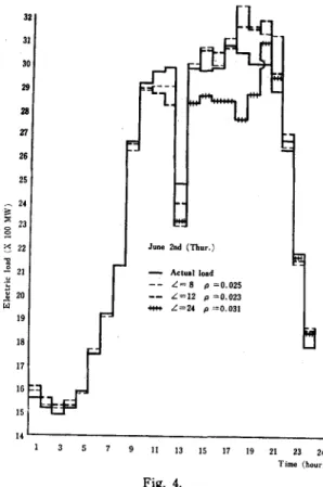
June 2nd (Thur.)

- - Predic.Jed load

- AetbaI load

p =0.023

M.x. error: 6%(to aetuallo.d)

14"":"""-::_-::--:-__________

--:-_

9 II U ~ U " n 23 U Time (hour)

Fig. 3.

After carrying experiments on the samples of the same company for about 30 days, we could have obtained the similar accuracy.

Now, we would like to discuss the problems of Cb) and Cc). In other word, we will examine how the number K of the characteristic mode functions and the length L of (18) influence to the prediction accuracy. Firstly, setting K constant, . we will examine the change of prediction accuracy due to L. Let us consider the variance of the prediction errors by means of the following fictitious model.

Power Load Prediction 135

x

(19) x(t)=

E

C,ifJt(t)+et,

;=1

where et is random variable and its mean and variance are zero and constant, respectively and;

Var (et) ==02 •

If the present time is To and prediction for load at time t is carried by means of eqn (10) and Ct are determined by means of (18), then the

variance Var (et) of the prediction error et.

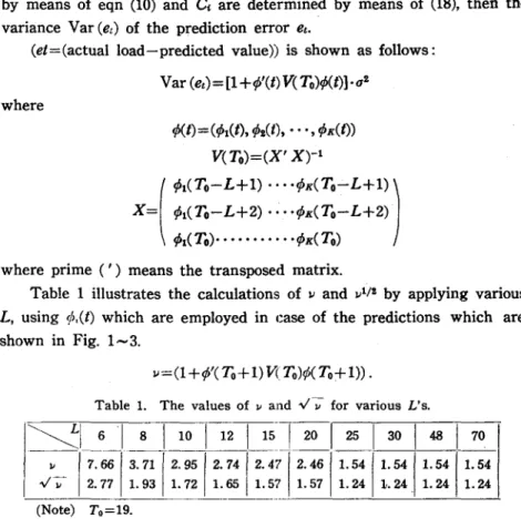
(et=(actual load-predicted value)) is shown as follows:

where

Var (et) = [1 +ifJ'(t) V( To)ifJ(t)]·02

ifJ(t)= (ifJl(t), ifJ2(t), ••• , ifJK(t)) V(To)=(X' X)-1

(

ifJl(To-L+l) ••• • ifJK(TO-L+l))

X= ifJl(To-L+2)··· ·ifJK(To-L+2) ifJl(To)··· ·ifJK(To) where prime (') means the transposed matrix.

Table 1 illustrates the calculations of 1.1 and 1.11/ 2 by applying various

L, using rp,(t) which are employed in case of the predictions which are shown in Fig. 1-3.

1J=(l+ifJ'(To+l)V(To)~(To+I)) .

Table 1. The values of lJ and ..;~ for various L's.

~I_!J

8

I

10

I

12

I

15

I

20

I

25

I

30

I

48

I

70

lJ 17.6613.71 12.9512.74 r 2.47 r 2.46 r 1. 54 r 1. 54 r 1. 54 r 1. 54

..;~ 2.77 1.93 1.72 1.65 1.57 1.57 1.24 1.24. 1.24 1.24 (Note) To=19.

As shown in the above, it is found that the variance of the prediction errors becomes larger as L become smaller and it becomes smaller as L

136 M. TOllama and K. Yamada

becomes larger. This is, however, based upon the assumption that X(t) depends upon the model of the eqn (19). In fact, the value, Ci changes daily, therefore, the prediction accuracy be.;omes worse if L is too large. This is illustrated in Fig. 4.

32 31 30 29 28 ?:1 26 25 _ 24

..

:;; 23 § ~ 22 11 ..2 21 .~ t 20 W June 2nd (Thur.) - Actual load L= 8 p =0.025 L=12 p =0.023 _ L=24 p =0.031

1.[

11 13 15 17 19 21 23 24 Time (hour) Fig. 4.

Fig. 4 shows that in case different pattern from the ordinaIIy one has occured, the prediction loses adaptability when L is large. In this figure it is found that the most favorable result is obtained from L=12. Next, we will examine by experiments what is appropriate for L

Power Load Predictloll

137

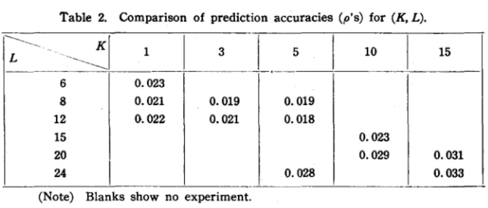
Table 2. Comparison of prediction accuracies (p's) for (K, L).

---

L

---

_--~ K[ I 3 5 10 15 6 0.023 8 0.021 0.019 0.019 12 0.022 0.021 0.018 15 0.023 20 0.029 0.031 24 0.028 0.033

(Note) Blanks show no experiment.

In this the load series are three days, May 29 th, June 1 st and 2 nd and p is calculated for the entire period of prediction. As noted in this,

K=5 and L=12,are most favorable. The reason why the results become

worse with increased K may be that L is necessary to become large in turn so that adaptability is lowered. In another examples, too, K=5 or its viciinity afford such a good result.

In the foregoing our experiments show that K=4-5 and L=12-15 are optimum. Furthermore, it is verified that the Farmer's Method falls into within all<;>wable errors against the load series.

In general, the most favorable value of K and L depends upon the load series and it may be decided theoretically if a proper model can be constructed for load. But in practice, it will be realistic to decide them by means of the experiments as described above.

4. Discussions to put this Method the Practical use (1) - Automatic check of load pattern

change-As described above, the Farmer's Method uses the characteristic mode function to predict electric load.

It is, therefore, necessary that load pattern at the time when the prediction is done is not so much different from that of the interval during whi~h characteristic mode functions are produced.

la8 M. TOllaltUJ and K. Yanuula

mode functions. It !?hould be noticed here that the change of a load pattern doesn't mean one or two unusual daily-patterns.

Then it is difficult and complicated for a system operator to find the change of daily load pattern because data are random.

Therefore, it is important to detect the change automatically. Es-pecially in the case that this prediction method is used in the on -line control system, automatic detection of pattern change is more necessary. One method to detect the pattern change automatically is described below.

Sample average value of Xm(t) at the time t, x(t), is expressed as eqn (20).

(20)

where xm(t) (m = 1, 2, ... , M) are sample functions which are used to calculate the characteristic mode functions.

Let

XCt)

be normalized so that an integral summation of normalized

value over interval (0, T) becomes a constant A. And let yet) be this normalized value, then

(21) y(t)

=(

A

I):

x(t)dt )X(t).

Now, when new daily load data x(t), (0::;;1::;; T) are given they are normalized as in eqn (22)

(22) j(t)=

(A

/~:

x (t)dt

)x(t)

(O::;;t::;; T).

Then square of the distance .between yet) and jet), D, is defined in eqn (23) and is considered as a index of pattern difference.

(23) D=

1:

(y(t)-x(t»2dt.

If D is large, it would be considered that x(t) is different from yet). Namely each pattern is different from another. On the contrary it can

Power Load Prediction 139 be considered that each pattern is same, if D is small.

But, using the above D to check pattern change, it is considered

that there is a pattern change even if x(t) is unusual only for one day. Therefore, to avoid such phenomena it should be considered to com-parey(t) with a normalized value which is obtained from weighted averaged value of past da~ involving x(t).

According to the exponentially smoothing method, we define weighte average value r(t) as follows:

(24) x'(t)=ax(t)+(l-a)x"(t) .

a is a positive number and smaller than 1, and x"(t) is a weighted average value obtained by eqn (24) using data of the previous day.

Furthermore, as initial value of x"(t) in eqn (24), we use iCt) in eqn (20)

Normalized form of x'(t) is:

(25)

j'Ct)

= ( A

11;

x'(t)dt)X'Ct)

COsts

T)

The new distance between yet) and x'(t) is defined as follows: (26) D=

~;

{y(t)-x'(t)}Zdt .

Then our method is as ""follows:

For some constant value w, we consider that the pattern changes if

Dc.w and it doesn't change if D<w.

There arises a problem to decide a and w. For this problem it is

more practical to decide them experimentally. Namely, using the series data of load of which a pattern changes on the way, daily calculation of D in eqn (26) is carried. Considering D's be time series, D must become large on the way if the pattern changes at that time.

But if a is very small, response to the pattern change is slow, and D would change fairly later than the actual pattern changes. If a is large, D would .response quickly to the unusual load pattern as described above.

Mo TOllama and K. Yamada

As an example, a result of experiments which are made using load data during April arid M~y is shown in Table 3. It must be noticed that the peak load time changes from the middle of April due to the length of day time.

From the above table, the following fact is apparent.

In the case of a=0.2 there is a large change of D on April 9 because

Table 3. Sequencies of D values a's.

~I

8/4

I

_{9/4 110/4114/4/15/4/16/4/17/4/21/4/22/4/23/4} 0.05 0 0 0 0 1 1 1 1 1 1 - - - -

- -

- - - -- - -0.1 0 1 1 1 2 2 2 2 2 2

- -

-0.2 1 4 3 3 6 3 4 4 5 6

~\24/4\28/4\30/4\

7/5 \8/5 \12/5\13/5\14/5\15/5 0.05 1 1 1 2 2 2 3

~

3 - -

-0.1 3 3 4 5 5 5 7 8 9

-0.2 7 5 7 10 10 9 13 18 14

(Note 1) Sat., Sun., Mon. and holidays are excluded. (Note 2) A=24. Figures show DXl000.

this day has an unusual pattern and it seems too sensitive.

Next in the case of a=0.05, D begins to change on May 9 th and this response is too slow.

In the case of a=O.l, it is most suitable case and when

w

is set to

0.003, D becomes larger than

w

on the appropriate day.

Several other experiments showed, that it is best when a and ware respectively set to about 0.1 and 0.003.

It is necessary to calculate the characteristic mode function again when D>w.

5. Discussions to put this Method to Practical use (2) - Dealing with the case containing trend

factor-Power Load Prediction 141

The case without trend factor is discussed above. But there may be a system whose load has trend factor even in a short term.

In such a case, it is not suitable to apply Farmer's Method directly to load prediction.

So it is necessary to modify the prediction system, considering trend factor.

A method is proposed, in which the Farmer's Method is involved. Briefly speaking, trend prediction is made by the Exponentially Smoothing Method, and the Farmer's Method is applied to trend-eliminated data, and then load prediction is obtained by combing these two predicted values.

And so, we assume that the Farmer's Method can be applied to predict trend-eliminated part.

First we define load pattern factor which is calculated from sample functions xm(t), (m=l, M) which are used to seek characteristic mode functions. That procedure is as follows:

For convenience later, we treat Xm(t) as a discrete function, and let

Xmn denote xm(t) at t=n, and n ranges from 1 to N, here N is the

number of sampling instants.

Now we estimate trend factor at nth time of m th day by the following moving average method:

(27)

where

mmn={YI_~ +2y,_~

+1+'"

+2Yt+~

-1

+YI+~}

N N

n="2'

2+

1, .. ·,N (m=l) N n=I,2,···, "2 n=I,2, ···,N (m=M) (m~l,M)

mmn: estimated trend factor

Ycm-1)N +n =Xmn

142 M. TOllanut and K. Yamada

here we assume

!:J

is even (e.g. N=24).

Next deviding Xmn by the estimated trend mrnn , we get Smn • Namely

(28)

Using Smn, load pattern factor, Si are defined as follows:

(29)

1 M ( N) 1 M-I ( N N )

si=-M_1

j"f/

Ji ;=1,2"

"'2

=M-1

j"f/

Ji

_;=2+

1

_{'2' ... ,}

N Using load pattern factor s,(;=1, N) described above, prediction is carried as follows:

First, we get characteristic mode functions from data Smn.

Let the calculated characteristic mode functions be

.,-·~k(t), (k=1, 2, ... ). Here t takes descrete value:

t=1,2, .. ·,N

Next, prediction of trend factor is done. When data up to some time r :y, ,y~-l' ... are given, trend factor is predicted by exponentially smoothing method. Namely, using estimated trend factor m'-l at time (r-1) and the latest data y" we estimate trend factor at time r by the following eqn (30):

(30)

Where Si is load pattern factor at time r and a is a positive number

which is smaller than 1. R~-l is estimated value of trend difference at time (r-1), and R, is obtained by eqn (31).

(31)

where

f'

is a positive number which is smaller than 1. And predicted value iit.+L of trend factor at time (r+L) is obtained as follows:

(32)

While prediction of trend-eliminated part is done by the Farmer's Method using characteristic mode functions calculated above as follows:

Power Load Prediction 143

(33) X'(p)=y(p)/mp

(p=r,r-l, ... ).

Thus prediction value y,+L of trcmd-eliminated part at time r+L is

obtained by eqn (34)

(34)

Final prediction value x" L of load at time r+L is obtained by eqn (35)

(35)

It is important to select initial values of m, and R, and smoothing

constant a and " optimally_

About initial values, we determined them as follows:

( i) Using sample data Xmn (m= 1, M; n= 1, N) with which charac-teristic mode functions are calculated, average load per day Vm for each

m is calculated as follows:

(36) J,lm= N 1

L:

N x mn(m=1,2,···, M)

n==l

( ii ) Initial value RO of R, is:

RO=(VM - V1)/(MN-N).

(iii) Initial value mO _of

m, is:

mO₌

V1 +W(MN--N/2).

About smoothing constants, some methods can be thought, for ex-ample, gradient method, simulation and son on. In our experiments, when they are about 0.1, good results were obtained.

Although experiments should be done using actual data which contain trend factor, we could not get such data. So fictitious data were pro-duced by adding various trend factor to data we used in the experiments

in chapter 3 and some experiments were done using them. Prediction was possible with almost same error as in chapter 3. But, to test our method with actual data remains as our subject.

144 M. Toyama and K. Yamada

6. Conclusion

The matterns discussed in this article can be summarized as follows: (1) We showed that the Farmer's Method can predict within the allowable accuracy using actual data.

(2) We proposed an automatic calculation method which shows when the recalculation of characteristic mode functions is to be carried, and experiments showed its practical usefulness.

(3) A method for predicting load containing trend was proposed. It combines the Farmer's Method and the Exponentially Smoothing Method and experiments showed good results.

On the other hand there are still many problems to be resolved in order to make the Farmer's Method more practical. Some of them are: (1) to improve prediction accuracy against unusual patterns. It is necessary to find out factors such as meteological components which affect the electric load and make rapid correspondense to such unusual conditions.

(2) to dispose against the loss of data.

(3) to speed up the calculation by the method of least squares . . Lastly, we would like to express our hearty thanks to Mr. H. Ogawa, Central Research Institute of Electric Power Industry, Dr. H. Kimura, and Dr.

J.

Baba, Mitsubishi Electric Corporation who kindly extended assistance.

REFERENCES

[1] R. G. Brown, "Smoothing, Forecasting and Prediction of Discrete Time Series", Prentice.Hall, 1962.

[2] P.R. Winters, "Forecasting Sales by Exponentially Weighted Moving Ave-rages" Management Science, 6, 3 (1960).

[3] E.D. Farmer, "A Method of Prediction for Non-stationary Process and its Application to the Problem of Load Estimation," Trans. I.F.A.C., (1963).

[4] G.T. Heinemann et al., "The Relationship between Summer Weather and

Loads-A Regression Analysis," PICA 1965 (Session IV).