第 4 章：Effects of Individual Resident Tax on the Consumption of Near-Retired Households in Japan1

第4 章：Effects of Individual Resident Tax on the Consumption of Near-Retired Households in Japan¹

Toshiyuki Uemura², Yoshimi Adachi³, Tomoki Kitamura⁴

2017/05/07

Abstract

We empirically investigate whether the Japanese individual resident tax causes a reduction in the consumption of near-retired households. In contrast to the income tax, the individual resident tax is levied on income from the previous year, and we found it has a negative effect on the consumption of three types of near-retired households: those who maintain regular employment, who move from regular to irregular employment, and who move from employment (regular, irregular, or self) to unemployment. Particularly, for the second type, the individual resident tax caused a larger reduction in household consumption.

Keywords: Individual resident tax, Consumption, Retirement, Life-Cycle model, Panel data JEL Classification Numbers: D12, D91, E21, H24, H31

1 We thank Hisahiro Naito, Yoko Yamamoto, Setsuya Fukuda, and participants in 2016 Japanese Economic Association spring meeting. This study is financially supported by a Japanese Health and Labour Sciences Research Grant

(H27-Statistics-General-004) from the Ministry of Health, Labour and Welfare of Japan

2 School of Economics, Kwansei Gakuin University, 1-155 Uegahara Ichiban-cho, Nishinomiya, Hyogo 662-8501, Japan.

3 Department of Economics, Konan University, 8-9-1 Okamoto, Higashinada-ku, Kobe 658-8501, Japan.

4 Finance Research Group, NLI-Research Institute,4-1-6. Kudan-kita, Chiyoda-ku, Tokyo 102-0073, Japan.

1. Introduction

We use individual data to empirically analyze whether the individual resident tax causes a reduction in the consumption of near-retired households. As we show in section 3, the Japanese individual resident tax is levied on income from the previous year. As a result, for near-retired households, where income decreases with age, this tax may be a constraining factor for consumption.

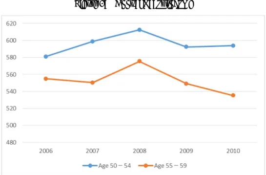
Figure 1 shows changes in the average value of worker income for the age cohorts 50–54 and 55–59, using national data on wages and salaries for working households, from the “Family Income and Expenditure Survey” (Statistics Bureau of the Ministry of Internal Affairs and Communication, 2017). As Figure 1 shows, worker income tended to decrease after its peak in 2008, and also as the retirement age approaches.⁵

[Insert Figure 1 here]

Even for households with regular workers, when income declines on a yearly basis, the individual resident tax may represent a relatively large cost. A tax on income from the previous year is a particular problem for households with workers who have moved from regular to irregular employment, as is for retired households. These types of households normally have lower income compared to households with regular workers. After a change in employment or during the first year of retirement, due to the cost of the individual resident tax, household disposable income decreases and consumption may also decline.

According to the life-cycle hypothesis, even if the individual resident tax is a tax on income from the previous year, for households able to anticipate this tax, the timing of the individual resident tax during retirement should not have an effect on consumption.

However, if such an effect is observed, either the life-cycle hypothesis does not hold true, an

5 Typically, the mandatory retirement age was 60 before 2005. In 2006, the elderly labor promoting law “Act on Stabilization of Employment of Elderly Persons” was implemented, and companies had to raise the mandatory retirement age from 60 to 62 in 2006, to 63 between 2007 and 2009, to 64 between 2010 and 2012, and to 65 after 2013, with some exceptions.

overreaction is occurring in response to the cost the individual resident tax represents during retirement, or households not being able to properly anticipate the cost of the individual resident tax. In this study, we clarify these possibilities through empirical analysis.

There are many opinions concerning the Japanese individual resident tax as a tax on income from the previous year. First, we introduce statements from organizations that believe that the individual resident tax should be a tax on income from the current year, as taxing income from the previous year has negative effects. For example, the Tax Commission of the Government of Japan (1968, p. 34) stated: “The resident tax is assessed based on income from the previous year. In other words, it is a tax on the previous year’s income. It is preferable that the tax be changed to apply to income from the current year, so that the tax is levied in response to the generation of income. This can be accomplished by bringing the point in time at which the tax is levied as close as possible to the point in time at which the income is generated. If such a transition is adopted, however, there will need to be changes to the way that withholding agents collect taxes, and a notification process for non-wage earned income will also need to be established. Therefore, further study is appropriate.” Additionally, the Tokyo-Chiho Certified Public Tax Accountants Association (2004, p. 46) stated: “… as it will be necessary for either withholding or year-end adjustment to occur, the administrative duties of those who pay wages will be increased.

There is room for more study concerning the adoption of a tax on current year income.

However, we advocate that a specific study be conducted with the aim of introducing a current year tax system at some point in the future.” Furthermore, the Tax Commission of the Government of Japan (2005, p. 13) affirmed that “the individual resident tax has been based on income from the previous year out of consideration for the administrative burden involved in paying taxes. However, essentially, for taxes on income, it is preferable that the point in time at which the income is generated and the point in time at which the tax is

levied be as close as possible. In recent years, the development of internet technologies, the diversification of employment structures, and changes in the economic climate have made the present moment an opportune time to conduct a study concerning the possibility of transitioning to a tax on current year income. Such a study should take the existing administrative burden of tax payers and others into account.”

The above organizations support transitioning the individual resident tax to a tax on current year income. Conversely, other organizations feel that such a transition would be inherently negative. For example, the National Association of Towns and Villages (2014, p.

9) stated that “concerning transitioning the individual resident tax to a tax on current year income, as such a transition would increase the administrative burden of municipalities and business owners, should be carefully studied.” Also, the Japan Chamber of Commerce and Industry (2015, p. 30) asserted that “the transition of the individual resident tax to a tax on current year income is being studied. However, for business owners, such a transition would require that businesses administer not only the income tax, but also the withholding or year-end adjustments associated with the individual resident tax. We oppose such a transition, as it would increase administrative burdens above current levels.” According to these organizations, the important questions are whether it is necessary to synchronize to as great a degree as possible the point in time income is produced to the point in time it is taxed, and whether a transition to a tax on current year income will increase the administrative burden of companies and local governments.⁶

Here, we move forward from these two problems, and present a novel issue that is more economic in nature. That is, we analyze whether the individual resident tax, as a tax on income from the previous year, causes a reduction in the consumption of near-retired

6 An example of an issue regarding transitioning to a tax on present year income is the synchronization of local tax benefits and liabilities. To coordinate the timing of local public services with the tax burden of the individual resident tax, the latter should transition to a tax on current year income.

households. We use panel data, covering retiring employees for this analysis.⁷ If the individual resident tax is causing a reduction in the consumption levels of near-retired households, then, it is also causing a reduction in household utility. If this is the case, a transition of the individual resident tax to a tax on income for the current year should be supported as a countermeasure. Alternatively, if the current system is to continue, policies to prevent the reduction of household consumption levels before and after retirement need to be studied.

In this paper, we use data from a large-scale government panel survey, carried out since 2005, which includes the behavior of individuals aged 50 to 59 in 2005. The information necessary to calculate the individual resident tax, including family structure, income, and employment status can be ascertained from this study. Total figures on household consumption are also included.

While controlling unobserved heterogeneity between individuals using a fixed effect model, we have estimated the effect of the individual resident tax on consumption.

The results show that, for households that maintained regular employment, for workers who moved from regular to irregular employment, and for workers who experienced a mix of regular, irregular, and self-employment, the individual resident tax had a negative effect on consumption. For households with workers who moved from regular to irregular employment, the individual resident tax caused a significantly larger reduction in household consumption.

The structure of this paper is as follows. Section 2 reviews previous research relevant to the contents of this paper. Section 3 contains an outline of the individual resident tax. Section 4 describes a household behavior model based on the life-cycle hypothesis, which provides the foundation for the empirical analysis contained in this paper. Section 5

7 We use data on individuals aged between 52 and 64. For the analyzed individuals, some workers continue to be employed, some face changes in employment type (e.g., full- to part-time), and some are retired.

presents an estimation model, and Section 6 explains the data and presents the results of our estimates. Section 7, the final section, compiles the results of our analysis and presents policy implications.

2. Literature Survey

If the life-cycle hypothesis holds, households should smooth consumption, as they can anticipate changes such as retirement and taxation. As this is an area of significant interest for empirical analysis, particularly regarding changes in consumption during retirement, a large body of previous research exists (e.g., Banks et al., 1998; Bernheim et al., 2001; Stephens Jr., 2003; Smith, 2004; Schwerdt, 2005; Hurst, 2008; Wakabayashi, 2008;

Battistin et.al., 2009; Kureishi, 2011; Aguila et al., 2011; Stephens and Unayama, 2012;

Hori and Murata, 2014; Kureishi and Yin, 2015; Li et al., 2015).⁸

This previous research primarily considers income shocks experienced during retirement, such as unanticipated early retirement, health deterioration, changes in dependents, or death of a spouse. It then subdivides consumer expenditure into different types, focusing on how low income individuals deal with financial constraints, and creates various mechanisms for actions such as identifying income brackets. Here, we focus on previous studies that examine whether household consumption responds to changes in income caused by the tax or social security systems, issues similar to the ones addressed in this paper. The following studies examine empirically whether different scenarios create a significant response in household consumption. For instance, Parker (1999) deals with the rate of income increase when the upper limits of social security tax are exceeded; Souleles (1999) looks at tax refunds, many received in the second quarter; Johnson et al. (2006) and Agarwal et al. (2007) deal with the 2001 tax rebates; and, along the same lines, Parker et al.

8 Hurst (2008) and Jappelli and Pistaferri (2010) perform extensive surveys in this respect.

(2013) deal with the 2008 rebates. For research conducted in Japan, Hori and Shimizutani (2002) analyze the effects of the 1998 reduction in income and individual resident taxes, and Hori et al. (2002) analyze the effect of regional shopping coupons. Most of this research indicates that changes in income caused by the tax and social security systems, such as tax rebates or tax reductions, result in a consumption increase. The analytical methods of these previous studies assume the life-cycle hypothesis, and use estimation methods based on the Euler equation for consumption. These studies also use individual data. Accordingly, the empirical analysis contained in this paper also uses estimation models based on the Euler equation and individual panel data that reflects the behavior of near-retired households. To verify the estimation model, we thus outline the individual resident tax system, which taxes income from the previous year, in the next section.

3. Outline of the Individual Resident Tax

Here, we explain the structure by which the individual resident tax is applied to income from the previous year. In Japan, the timing of the income tax (a national tax), levied on income from the current year, is different from the timing of the individual resident tax (a local tax).

Person H, a salaried employee, earns income from working at Company F for a period of one year, from January 1 to December 31 of Year 1. Person H is paid wages by Company F for Year 1 between January and December, which withholds income tax from Person H’s wages. When the year-end adjustment occurs in December, Person H pays income tax owed to the tax office in proportion to the amount of tax that has been withheld.

Accordingly, the process of collecting the income tax, a tax on income from the current year, is concluded within the current year by means of the year-end adjustment.

When Year 2 begins, Company F notifies Municipality M, the municipality in

which Person H lives on January 1, Year 2, of Person H’s wages for Year 1. Municipality M calculates Person H’s individual resident tax liability, and asks Company F to withhold income from Person H’s wages until around May of Year 2. Company F, having received the withholding request, withholds the monthly amount of individual resident tax from June of Year 2 to May of Year 3 by deducting it from Person H’s wages, and pays the tax to Municipality M. The individual resident tax paid to Municipality M includes municipal and prefectural resident taxes. In this way, prefectural resident taxes are paid to the prefecture through the municipality. The process of collecting the individual resident tax extends in Year 2. The problem addressed in this paper is whether the individual resident tax affects the consumption levels of near-retired households.⁹

For salaried employees, the amount of the individual resident tax is calculated in the following manner. Salaried income deductions are calculated using salaried income from the previous year and, by subtracting these deductions from salaried income, employment income is obtained. Employment income deductions are calculated using household family structure and social security payments. These employment income deductions are then subtracted from employment income, thus yielding the taxable income.

A tax rate of 10% is applied to taxable income (4% prefectural and 6% municipal tax).

Therefore, the amount of individual income tax is obtained.

For example, using the 2016 tax structure, let us compare the income and individual resident taxes for a single, salaried employee earning JPY 4 million. If only the salaried income deduction, basic deduction, and JPY 400,000 social security payment deduction are applied, the amount of income tax will be JPY 95,900, and the individual

9 Active salaried workers can choose a special collection of the individual resident tax. The special collection is a withholding method in which tax is withheld from a worker’s salary by their employer. However, after retirement, households switch from special to general collection. In general collection, an individual must directly pay individual taxes to the municipality in which he/she lives. Even households whose income has decreased due to retirement must pay their individual resident tax.

resident tax JPY 195,500.¹⁰ That is, the individual resident tax will be greater than the income tax, a fact that has a significant effect on consumption by itself.¹¹

Generally, a reduction in income with age is observed for salaried employees close to retirement. As a result, the individual resident tax, which is calculated using the higher earnings from the previous year, may affect consumption in the current period. Furthermore, when a worker moves from regular employment to irregular employment, the change in employment status is usually accompanied by a large income reduction.¹² As such, we empirically study what types of effects the individual resident tax has on the consumption of retirement-age households with reduced income.¹³

4. Household Behavior According to the Life-cycle Hypothesis

Here, we propose the model that forms the basis of our analysis. Let t represent time. We assume that a household has a time-sealable utility, u, which is a function of uncertain consumption, Ct. Then, we can express the households’ expected utility, V, as follows:

1 , 1

where ρ is the time preference. Additionally, we assume that ^’ 0、 0. Next, household budget constraints are assumed to be as follows:

1 , 2

where savings are At, income is Yt, the amount of tax owed is Tt, and the interest rate is r.

10 From this figure for individual resident tax, JPY 77,700 represents the prefectural and JPY 117,800 the municipal tax.

11 The circumstance by which the individual resident tax became higher than the income tax is the tax source transition implemented in 2007. The scale of this transition was around JPY 3 trillion.

12 Households whose income has decreased and have switched to general collection immediately following retirement can expect a large tax burden.

13 A lump-sum retirement bonus is paid when a worker retires. However, the individual resident tax that should be paid in the next fiscal year is normally withheld from this sum, and thus paid in the current year. Retirement money is therefore not subject to the next year’s individual resident tax, and the effect of this tax on the bonus is limited.

Solving the expected utility maximization problem using equations (1) and (2), we obtain the Euler equation below:

1

1 . 3

Additionally, we specify utility at a point in time, u(Ct), in constant relative risk aversion (CRRA) form:

u 1 , 4

where the relative risk aversion is γ, elasticity of intertemporal substitution 1/γ, and . Subsequently, we assume that consumption C follows a log normal distribution (lnC～N(μ,σ²)). Then, if we assume that the interest rate, r, and the time preference, ρ, are sufficiently small, the Euler equation can be expressed as follows:

1

1 ＝ . 5

If we take the log and organize the above expressions, we obtain the following equation:

＝ ¹

2 ln , 6

where ≡ . Using equation (6) and based on the relationship between the magnitude of the interest rate, r, and the time preference ratio, ρ, changes in household consumption, ln ln , can be determined. If the life-cycle hypothesis holds, factors contributing to changes in income, such as the individual resident tax, should not affect consumption Ct. However, if households cannot anticipate changes in income due to the individual resident tax, there will be an effect on consumption Ct. Even if changes in income are anticipated, there may be an overreaction in household consumption. If for some reason consumption smoothing cannot be performed, there will also be an effect on

household utility levels. Accordingly, we address whether and to what degree changes in individual resident tax affect household consumption Ct. Additionally, we analyze the effect of the income tax on consumption and compare it to the effects of the individual resident tax.

In the next section, we construct an estimation method based on equation (6) and perform the empirical analysis.

5. Estimation Model and Data

We estimate the following regression model from equation (6) in the previous section:

ln _, ∙ _, ∙ _, ∙ _, ∙ _,

∙ _, , 7

where the household is denoted by i, the year is t, the difference in the individual resident tax is , changes in employment status are Cemp j 1, ⋯ , 4 , the control variable is , the regression coefficient is β, the fixed effect is δ, and the error term is ε. ∙ is the indicator function, and _, ∙ _, the interaction term. The response variable is the change in consumption, ln _, ≡ ln _, ln _, . We also use four categories of employment status. These are regular (full-time), irregular (part-time, temporary, by commission), self-employed, or unemployed. The variable that expresses changes in employment status is defined as follows. For years in which employment status does not change from regular, Cemp 1; if employment status changes from regular to irregular, Cemp 2 ; if employment status changes from employed (regular, irregular, or self-employed) to unemployed, Cemp 3; and for all other changes to employee status, Cemp 4. The base case for the following estimation results is Cemp 1.

It is possible to differentiate between unemployment due to involuntary and voluntary job loss (retirement). However, in analyzing the effects of the individual resident tax, as both scenarios imply that individuals are not working and as discerning between these scenarios would make the sample size unusably small for some years, we have conducted the analysis without making this distinction. The reason for not taking the logarithm of the difference in individual resident tax, , is that, if a household’s income is below a fixed amount, their individual resident tax will be zero.

Based on the estimation results from equation (7), we examine whether the individual resident tax affects consumption. If the life-cycle hypothesis does hold, the individual resident tax should not affect consumption, and we verify null hypothesis 1:

E ∆

∆ 0, 1, 2, 3, 4. 8

Equation (8) verifies whether the average marginal effect (AME), which represents the changes in consumption with respect to the changes in the individual resident tax, is zero.

We evaluate AME using each possible change in employment status ( ). If the null hypothesis is rejected, changes to the individual resident tax affect consumption, which contradicts the life-cycle hypothesis. Particularly, if AME is negative, the individual resident tax causes a decrease in consumption.

Subsequently, if the life-cycle hypothesis does not hold (if the null hypothesis above is rejected), we verify whether the effect the individual resident tax has on consumption varies with employment status. For example, if AME for individuals who moved from regular to irregular employment is smaller than for individuals who maintained regular employment (i.e., the negative value is larger), we can conclude that the variations in the individual resident tax were larger for those whose employment status changed (i.e.,

who moved from regular to irregular employment). Therefore, we verify null hypothesis 2:

E ∆

∆ E ∆

∆ 1 0, 2, 3, 4. 9

Equation (9) determines whether the difference between the AME of individuals whose employment status did not change from regular employment and of individuals whose employment status did change is zero. If this null hypothesis is rejected, variations in the individual resident tax affect consumption differently depending on changes to employment status. Here, we are particularly interested in the difference between situations in which workers moved from regular to irregular employment (Cemp 2) and those in which workers maintained regular employment (Cemp 1), and also in the difference between situations in which workers went from being employed to unemployed Cemp 3 and those in which workers maintained regular employment. If these differences are negative, variations in the individual resident tax caused a greater decrease in the consumption of workers whose employment status changed than in the consumption of workers who maintained regular employment. The reason for the existence of the interaction term in equation (7) is to estimate equations (8) and (9). We have also conducted analysis on the income tax, in which we replace _, from equations (7), (8), and (9) with the difference in income tax, _, .

Further, we use a fixed effect model to estimate equation (7). Concerning the relationship between variations in the individual resident tax and changes in consumption, the estimations may be mutually dependent. In other words, there is a possibility of endogeneity (simultaneous determinacy). For example, workers with a specific skill may earn comparatively higher wages and thus pay a higher individual resident tax. If the income and individual resident tax for such a worker decrease due to changes in

employment, consumption may drop dramatically. On the other hand, workers with no specific skills may not have paid high individual resident taxes to begin with. For them, the effects of the individual resident tax at retirement will likely be limited. However, bias may exist in estimates of the relationship between variations in individual resident tax and changes in consumption that do not consider these types of scenarios. For estimation methods that consider this type of endogeneity, in instances where cross-sectional data are used, instrumental variables may be employed. Furthermore, the use of panel data allows the use of a fixed effects model, in which heterogeneity between individuals that is time invariant is captured by a fixed effect, .¹⁴ The fixed effect δ can be correlated with

∆ .

The panel data used in the paper is individual data from the “Longitudinal Survey of Middle-aged and Elderly Persons,” conducted by the Ministry of Health, Labour and Welfare. This survey was first conducted at the end of October in 2005 for individuals aged 50 to 59. The data used for the analysis in this paper is from 2007 to 2010. Data until 2006 was not used because the sources of tax revenue shifted in 2007 to depend less on the income tax, a national tax, and more on the individual resident tax (Ministry of Internal Affairs and Communication, 2009). If we use both the data before and after the shifting of tax revenue sources in 2007, it would not be possible to determine whether effects on income were due to an increase in the individual resident tax caused by the shifting tax revenue or due to the fact the individual resident tax is a tax on the previous year’s income.

Therefore, we have only used data from after the tax revenue shift. Due to the shifting of tax revenue sources, the income tax was reduced, while the individual resident tax increased.

14 However, even if this type of endogeneity is considered as a fixed effect, heterogeneity between individuals that varies with time may persist. In such cases, a fixed-effects regression with instrumental variables can be used. This method deals with heterogeneity between individuals that does not change over time using a fixed effect and with heterogeneity between individuals that does change over time using instrumental variables. However, in this paper, we only perform estimates based on a fixed effects model. Usually, it is difficult to find appropriate instrumental variables. However, this is an issue for future study.

Accordingly, the effect of the individual resident tax on individuals of near-retirement age should be larger following the shift.¹⁵

Of the 25,157 men and women who responded to the survey from 2005 to 2010, we screened 5,298 regularly employed, married men in 2007. Any individual whose income in 2007 was zero or missing was excluded, as were those whose employment status has been missing at any point since 2008. Additionally, regarding variables with positive values, values that exceeded three standard deviations have also been excluded as outliers. The standard deviation is computed excluding zero values. We have limited our analysis to men because, in the generation being studied, many households live primarily on income they earn. As a result, when focusing on men, the effects of the individual resident tax and of changes in employment status should be more pronounced. We also restricted our analysis to married individuals because the income and consumption trends of married and unmarried individuals differ significantly, to the effect that each group would need to be analyzed individually. However, the sample of unmarried individuals was not large enough for analysis.

The variables used in this paper were produced in the following manner. The presence of double quotations indicates data entries from the survey. Household consumption, C, is “Household expenditures” (monthly). Household individual resident tax, , was calculated using the following procedure. First, if an individual “Has income,”

then the “Amount of income in the last month apart from public pension income” was multiplied by 12. As this figure does not include bonuses, the income from wages including bonuses was obtained by multiplying the base wage by a bonus factor. This bonus factor

15 For example, according to the National Tax Agency (2006), a family consisting of a husband, wife, and two children with earnings of JPY 5 million would have paid JPY 119,000 in income tax and 76,000 in individual resident tax before the tax revenue source shift. After the shift, an income tax of JPY 59,500 (50% less than before the reforms) and individual resident tax of JPY 135,500 (78% more) would have been paid. However, the total amount of taxes paid before and after the reform remained similar.

was computed as a ratio of “Annual special cash earnings” on “Contractual cash earnings”

from the “Basic Survey on Wage Structure (Ministry of Health, Labour and Welfare, 2010)”.

These figures differ based on employment status, age group, industry, and gender.

Applying the individual resident tax schedule to income from the previous year, we calculated the amount of individual resident tax, , as follows. Taking the household’s situation into account, we calculated taxable income by applying the following deductions:

earned income deduction (at least JPY 650,000), basic deduction (JPY 330,000), spouse deduction (JPY 330,000), deductions for dependents (JPY 330,000), and the social security fee deduction, calculated using the simple calculation equation from the Ministry of Finance (Ministry of Finance Policy Research Institute, 2016). By applying a 10% tax rate to this figure, we obtained the amount of individual resident tax. Additionally, for subjects recorded under “Has income,” because they receive a pension, we multiplied the “Amount of public pension received” (bi-monthly) by 6. We calculated the individual resident tax from the pension income of previous year as well, considering the public pension deduction.

For , the amount of income tax, we calculated this figure by applying the income tax schedule to income earned in the current year.

Regarding controlled variables, we used dummy variables to represent the following conditions: a spouse with earned income, a dependent child (under 24 living with parents), age above 60, housing (owning a house, renting, other). We also used objective changes to health condition (positive values mean subjective improvement of health), and year dummies.

6. Estimation Results

Appendix A shows the characteristics of the sample used in this paper. Panel A shows changes in age. The sample was between ages 52–61 in 2007 and 55–64 in 2010.

Panel B shows changes in sample size by employment status. In 2007, all analyzed subjects were regular employees, a portion of the sample moving to irregular employment, self-employment, or unemployment over time. As such, the number of regular employees decreased, and the number of those irregularly employed and unemployed increased. Panel C shows variations in the sample size through changes in employment status (Cemp 1 4). Cemp 1, which denotes maintaining regular employment, is the most common. Our interest is the change of consumption for Cemp 2, which denotes a change from regular to irregular employment, with a total number of 1,400 observations, and that of Cemp 3, which denotes a change from employment to unemployment, with a total number of 769 observations. Table 1 contains the descriptive statistics for the data used in our analysis, including the mean values and standard deviations for the pooled data for 2008–2010.

[Insert Table 1 here]

Table 2 shows changes in mean, standard deviation, and sample size for consumption, individual resident tax, and income tax by employment status, respectively.

Ranked by total consumption, regular employees are the highest with JPY 4.04 million per year, followed by irregular employees with 3.34 million and the unemployed with 3.23 million. Therefore, consumption differs due to changes in employment status. According to total individual annual resident tax, regular employees pay the most at JPY 317,000 (on average), and the self-employed pay a similar amount. On the other hand, irregular employees pay around JPY 169,000. The unemployed, who earn no wages, are still obliged to pay an average individual resident tax of around JPY 150,000, which is levied on the previous year’s income. Regarding total annual income tax, the regularly employed pay the highest income tax at around JPY 410,000. As the income tax is on current year income, the unemployed pay only JPY 40,000, considerably less than either irregular employees or the self-employed.

[Insert Table 2 here]

Panel A of Appendix B shows a scatter plot and histogram of the main analyzed variables: changes in individual resident tax (∆LT) and in consumption (∆lnC). This figure contains all analyzed data. The horizontal axis is ∆LT and the vertical axis is ∆lnC, the histogram showing a roughly symmetrical distribution for both variables. The straight line on the scatter plot represents the fitted values according to ordinary least squares (OLS) regression, which exhibit an inverse relationship (that is, as ∆LT increases, ∆lnC decreases). Panel B shows scatter plots according to changes in employment status (Cemp).

The fitted values for Cemp 1,2,3 according to the OLS regression, which are represented by straight red lines, trend downward as they move to the right. Panel A of Appendix C shows a scatter plot and histogram representing the changes in income tax (∆NT) and consumption (∆lnC). The fitted values, according to the OLS regression, within the scatter plot exhibit a positive relationship (that is, as ∆NT increases, ∆lnC increases).

Accordingly, the individual resident and income taxes may have different effects on consumption changes.

Table 3 shows the estimated results of the fixed effect model. As correlation in the behavior within survey responders was predicted, we estimated clustered standard errors at the respondent level.¹⁶ Column (1) shows the estimated results for changes in individual resident tax (∆LT), whose coefficient is negative and statistically significant, as is for Cemp 2 and Cemp 3, the variable that represents changes in employment status.

Regarding the interaction term, ∆LT Cemp 2 is both negative and statistically significant.

[Insert Table 3 here]

Panel A of Figure 2 shows the estimated results graphically, based on Column (1)

16 Typically, a clustered standard error is larger than a robust standard error that considers heteroscedasticity, making it harder for variables to achieve significance.

of Table 3. The vertical axis represents the predicted values of ∆lnC, and the horizontal axis represents ∆LT evaluated at ∆LT 15, 10, ⋯ ,10 (i.e., the unit is JPY 10,000). The slope of each line corresponds to the AME in equation (8). If the life-cycle hypothesis holds,

∆lnC should not respond to ∆LT, and the slope should be flat (i.e., the marginal effect should be zero). Additionally, as equation (7) contains no second-order terms related to

∆LT, the AME (slope) is the same regardless of which ∆LT value it is evaluated at. In Panel A of Figure 2, the slope of Cemp 1 is gently negative. The slopes of Cemp 2 and Cemp 3 are also negative. The differences between the slopes of each line correspond to the differences between the AMEs in equation (9). In contrast to the gentle slope of Cemp 1, the slope of Cemp 2 is steeper. In other words, the individual resident tax is expected to have a larger effect for workers moving from regular to irregular employment than for those who maintain regular employment.

[Insert Figure 2 here]

Table 4 shows the test results of the null hypotheses, which deal with marginal effects. Panel A shows marginal effects related to ∆LT. The top section of the table shows the test results for null hypothesis 1. Here, the marginal effect is equivalent to the slopes of the lines from Figure 2. The marginal effects for Cemp 1,2,3 are negative and statistically significant, thus rejecting null hypothesis 1. A tendency towards the decrease of consumption due to the individual resident tax is shown, but the results are not consistent with the life-cycle hypothesis.

The lower part of Panel A in Table 4 shows the test results for null hypothesis 2, a hypothesis dealing with differences in the marginal effect. The differences are equivalent to the differences in the slopes of the lines in Figure 2. For Cemp 2 Cemp 1 , the null hypothesis is rejected, implying that the individual resident tax had a greater effect on consumption for those workers whose employment status changed from regular to irregular

employment than for those who maintained regular employment. On the other hand, Cemp 3 Cemp 1 is not significant. The individual resident tax did not reduce consumption more for workers who retired than for workers who maintained regular employment.

[Insert Table 4 here]

Column (2) of Table 3 shows the estimated results for changes in income tax (∆NT), whose coefficient is positive and statistically significant. None of the Cemp coefficients are significant. The interaction term ∆NT Cemp 3 is positive and statistically significant.

Panel B of Figure 2 shows the estimated results graphically, based on Column (2) of Table 3.

The slopes of Cemp 1,2,3 are all positive.

Panel B of Table 4 shows the results of testing the null hypothesis for the significance of the marginal effect. The top part of the table shows the test results of null hypothesis 1. The marginal effect of Cemp 1,2,3 is positive and statistically significant, and the null hypothesis is rejected. This result is not consistent with the life-style hypothesis.

The income tax being levied on present year income, it has a high correlation with income.

These results imply that when income decreases, it causes a decrease in consumption. The lower part of Panel B in Table 4 shows the test results of null hypothesis 2, which is related to differences in marginal effect. Differences in the marginal effect correspond to the differences of slopes of the lines in Figure 2. For Cemp 3 Cemp 1 , null hypothesis 2 is rejected. As such, the income tax had a larger effect on consumption for workers who moved from employment to unemployment than for those who maintained regular employment.

The results of the analysis above show that the individual resident tax has a negative effect on consumption for individuals who maintain regular employment, for those whose employment status changes from regular to irregular employment, and for those who

go from being employed to being unemployed. Particularly, for households with workers whose employment status changes from regular to irregular employment, a larger negative effect on consumption is shown. As such, households may be unable to predict the amount of individual resident tax at retirement. Alternatively, they may be able to predict it, and yet still feel the need to reduce their consumption levels by a relatively large degree. Our results indicate that the individual resident tax prevents near-retired households from smoothing consumption and has a negative effect on household utility. On the other hand, the income tax has a positive effect on consumption. This is likely because a decrease in income results in a lower income tax.

7. Conclusion

We conducted an empirical analysis using individual data on whether the Japanese individual resident tax, a tax on income from the previous year, causes a decrease in consumption for near-retired households. If households perform consumption as predicted by the life-cycle hypothesis and are able to anticipate individual resident tax as a tax on income from the previous year, the amount of individual resident tax they need to pay after retirement should not have an effect on household consumption. Our analysis uses individual data from the “Longitudinal Survey of Middle-aged and Elderly Persons,”

conducted by the Ministry of Health, Labour and Welfare. According to our results, which estimated changes in consumption for households with workers whose employment status remains regular, workers whose employment status changes from regular to irregular employment, or workers who move from employment to retirement, the individual resident tax causes a reduction in the consumption. Particularly, for workers whose employment status changes from regular to irregular employment, household consumption reduces even more. On the other hand, no such tendency was observed for the income tax. This means

that households were unable to anticipate the individual resident tax at retirement, or even for households able to anticipate it, they had to decrease consumption levels. The fact that the individual resident tax had a negative effect on variations in household consumption means that it inhibited the smoothing of household consumption and had a negative effect on household utility.

From the results above, we can conclude that the individual resident tax system, in which income from the previous year is taxed, is not a desirable system, because of its negative effect on consumption levels. The Tax Commission of the Government of Japan (1968, 2005) and Tokyo-Chiho Certified Public Tax Accountants Association (2014) have expressed the view that the individual resident tax should transition to a tax on present year income. The fact that the current system has a negative effect on household consumption supports the study of such a transition. Alternatively, if the individual resident tax is to be maintained as a tax on income from the previous year, some sort of countermeasure is necessary to prevent household consumption from declining. For example, for employees yet to retire, awareness of the fact that the individual resident tax is a tax on income from the previous year could be increased. Additionally, a pre-payment system could be established for the payment of this tax by those of retirement age. Finally, the individual resident tax incurred in the year immediately after retirement could be paid before retirement.

The analysis in this paper has certain limitations. First, we only considered the total amount of consumption and, as a result, employment-related spending has been included.

As such, it is possible that consumption decreased because employment status changed.

Additionally, as the data used for annual consumption in our analysis are computed from the monthly consumption on October of each year recorded in the survey, additional consumption in months when bonuses are paid or during the holiday season is not included.

This is due to the limitations of the survey data used in this paper. In the future, we would like to analyze different types of consumption subdivisions. Furthermore, the figures for income and individual resident tax used in this paper have been estimated by applying the tax system based on information such as income, employment status, and family structure from the survey. As such, it is possible that these figures differ from the actual amount of individual resident and income tax paid. If it had been possible to use actual data on these taxes, a more precise analysis could have been performed. This is an issue for future study.

Acknowledgements

We thank Kunio Nakashima, Hisahiro Naito, Yoko Yamamoto, Toru Kobayashi, Setsuya Fukuda, Wataru Kureishi, and the participants to the 2016 Japanese Economic Association spring meeting. This study was financially supported by the Health and Labour Sciences Research Grant of Japan (H27-Statistics-General-004). We would like to thank Editage (www.editage.jp) for English language editing.

References

Agarwal, S., C. Liu and N. S. Souleles (2007) “The Reaction of Consumer Spending and Debt to Tax Rebates: Evidence from Consumer Credit Data”, Journal of Political Economy, Vol. 115, No. 6, pp. 986–1019.

Aguila, E., O. Attanasio, and C. Meghir (2011) "Changes in Consumption at Retirement:

Evidence from Panel Data”, Review of Economics and Statistics, Vol. 93, No. 3, pp. 1094–1099.

Banks, J., R. Blundell and S. Tanner (1998) “Is There a Retirement-Savings Puzzle?”, American Economic Review, Vol. 88, No. 4, pp. 769–788.

Bernheim, B. D., J. Skinner and S. Weinberg (2001) "What Accounts for the Variation in

Retirement Wealth among U.S. Households?”, American Economic Review, Vol.

91, No. 4, pp. 832–857.

Battistin, E., A. Brugiavini, E. Rettore and G. Weber (2009) “The Retirement Consumption Puzzle: Evidence from a Regression Discontinuity Approach”, American Economic Review, Vol. 99 No. 5, pp. 2209–2226.

Haider, S. J., and M. Jr. Stephens (2007) “Is There a Retirement-consumption Puzzle?

Evidence Using Subjective Retirement Expectations”, Review of Economics and Statistics, Vol. 89, No. 2 , pp. 247–264.

Hori, M., C. Hsieh, K. Murata, and S. Shimizutani (2002) “Did the Shopping Coupon Program Stimulate Consumption? Evidence from Japanese Micro Data”, ESRI Discussion Paper Series, No. 12.

Hori, M., and K. Murata (2014) “Is there a Retirement Consumption Puzzle in Japan?

Evidence based on Panel Data on Households in the Agricultural Sector”, ESRI Discussion Paper Series, No. 308.

Hori, M., and S. Shimizutani (2002) “Micro Data Studies on Japanese Tax Policy and Consumption in the 1990s”, ESRI Discussion Paper Series, No. 14.

Hurst, E. (2008) “The Retirement of a Consumption Puzzle”, National Bureau of Economic Research, Working Paper 13789.

Japan Chamber of Commerce and Industry (2015) “An Opinion Concerning Revisions of the Tax System for Fiscal Year 2016”,

http://www.jcci.or.jp/sangyo/tax/20150916_zeiseiiken.pdf (in Japanese).

Jappelli, T. and L. Pistaferri (2010) “The Consumer Response to Income Changes”, Annual Review of Economics, Vol. 2, pp. 479–506.

Johnson, D.S., A. Parker and N. S. Souleles (2006) “Household Expenditure and the Income Tax Rebate of 2001”, American Economic Review, Vol. 96, No. 5, pp. 1589–1610.

Kureishi, W. (2011) “The Effect of Unexpected Events on the Standard of Living and Well-being of Retirees”, The Quarterly of Social Security Research, Vol. 46, No.

4, pp. 368–381.

Kureishi, W. and T. Yin (2015) “Decline in Consumption Expenditures after Retirement Using Japanese Micro Data (JSTAR)”, RIETI Discussion Paper Series, 15-J-001.

Li, H., X. Shi, and B. Wu (2015) "The Retirement Consumption Puzzle in China", American Economic Review, Vol. 105, No. 5, pp. 437–441.

Ministry of Finance Policy Research Institute (2016) “Tax Report: Annumal Comparizon of Income Tax”, Ministry of Finance Statistics Monthly, Vol. 769,

http://www.mof.go.jp/pri/publication/zaikin_geppo/hyou/g769/769.htm (in Japanese).

Ministry of Health, Labour and Welfare (2010) “Basic Survey on Wage Structure”, http://www.mhlw.go.jp/english/database/db-l/wage-structure.html.

Ministry of Internal Affairs and Communications (2009) “An Overview of the Trinity Reform”,

http://www.soumu.go.jp/main_sosiki/jichi_zeisei/czaisei/czaisei_seido/zeigenijou 2_1.html (in Japanese).

National Association of Towns & Villages (2014) “Requests Related to Government Policy and Budget Formation for Fiscal Year 2015”,

http://www.zck.or.jp/activities/260703/2.pdf (in Japanese).

National Tax Agency (2006) “Beginning in 2007, the Income Tax and Individual resident tax Will Change (Tax Revenue Shifting)”,

https://www.nta.go.jp/sonota/sonota/osirase/topics/data/h18/5383/01.htm (in Japanese).

Parker J. A. (1999) “The Reaction of Household Consumption to Predictable Changes in

Social Security Taxes”, American Economic Review, Vol. 89, No. 4, pp. 959–973.

Parker J. A., N. S. Souleles, D. S. Johnson and R. McClelland (2013) “Consumer Spending and the Economic Stimulus Payments of 2008”, American Economic Review, Vol.

103, No. 6, pp. 2530–2553.

Schwerdt, G. (2005) “Why does Consumption Fall at Retirement? Evidence from Germany”, Economics Letters, Vol. 89, No. 3, pp. 300–305.

Smith, S. (2004) “Can the Retirement Consumption Puzzle be Resolved? Evidence from UK Panel Data,” Institute for Fiscal Studies Working Paper, 04/07.

Souleles N. S. (1999) “The Response of Household Consumption to Income Tax Refunds”, American Economic Review, Vol. 89, No. 4, pp. 947–958.

Statistics Bureau of the Ministry of Internal Affairs and Communication (2017) “Family Income and Expenditure Survey”,

http://www.stat.go.jp/data/kakei/2.htm#new.

Stephens Jr., M. (2003) “’3rd of the Month’: Do Social Security Recipients Smooth Consumption between Checks?”, American Economic Review, Vol. 93, No. 1, pp.

406–422.

Stephens Jr., M. and T. Unayama (2012) “The Impact of Retirement on Household Consumption in Japan”, Journal of Japanese and International Economies, Vol.

26, No. 1, pp. 62–83.

Tax Commission of the Government of Japan (1968) “Report on the State of Long-term Tax System”,

http://www.soken.or.jp/p_document/zeiseishousakai_pdf/s4307_tyoukizeiseinoari katahoka.pdf(in Japanese).

Tax Commission of the Government of Japan (2005) “Discussion Points Related to the Individual Income Tax”,

http://www.soken.or.jp/p_document/zeiseishousakai_pdf/h1706_kojinsyotokukaz ei.pdf (in Japanese).

Tokyo-Chiho Certified Public Tax Accountants Association (2014) “Opinion Paper on Revisions of the Tax System for Fiscal Year 2015”,

http://tochizei.or.jp/zeiseikaisei/pdf/h27.pdf (in Japanese).

Wakabayashi, M. (2008) “The Retirement Consumption Puzzle in Japan”, Journal of Population Economics, Vol. 21, No. 4, pp. 983–1005.

Figure 1: Annual Labor Income

Note: This graph shows the average national wage salaries for worker’s households by age cohort for the head of household, as per the “Yearly Average of Monthly Receipts and Disbursements Per Household”

from the “Family Income and Expenditure Survey,” conducted by the Statistics Bureau of the Ministry of Internal Affairs and Communication. The units are expressed in JPY 10,000 per year.

Figure 2: Estimation Results for Individual Resident and Income Taxes

Panel A: Relationship Between the Estimated Results for ΔLT and Δln Consumption (Delta ln C)

Panel B: Estimation Results for the Relationship Between ΔNT and Δln Consumption (Delta ln C)

Note: This figure shows the relationship between the change of each tax and the Δln of consumption based on the estimated results in Table 3.

Table 1: Descriptive Statistics

Note: The Cemp variable expresses changes in employment status: Cemp = 1 represents maintaining regular employment, Cemp = 2 represents moving from regular to irregular employment, Cemp = 3 represents moving from employment (regular, irregular, or self) to unemployment, and Cemp = 4 represents all other changes. (d) represents a dummy variable.

Variable Unit N Avg. S.D. Min Max

Annual consumption (C) 10,000 JPY 20,227 392.17 (180.08) 0 1,716.0

ΔLn C 14,359 -0.029 (0.310) -1.11 1.0

Annual labor income 10,000 JPY 17,925 584.32 (434.47) 0 4,613.7

Annual pension 10,000 JPY 20,862 14.60 (44.04) 0 300.0

Annual local tax (LT) 10,000 JPY 18,237 29.18 (32.64) 0 398.9

Annual national tax (NT) 10,000 JPY 18,161 35.65 (86.86) 0 1,312.0

ΔLT 10,000 JPY 11,853 -0.866 (12.96) -67.51 65.50

ΔNT 10,000 JPY 10,905 -4.140 (25.07) -210.83 202.33

Employment = Regular (d) 21,192 0.822 (0.382) 0 1

Employment = Irregular (d) 21,192 0.100 (0.300) 0 1

Employment = Self-emp. (d) 21,192 0.021 (0.144) 0 1

Employment = Unemployed (d) 21,192 0.057 (0.231) 0 1

Cemp = 1 (d) 15,894 0.742 (0.437) 0 1

Cemp = 2 (d) 15,894 0.088 (0.283) 0 1

Cemp = 3 (d) 15,894 0.050 (0.218) 0 1

Cemp = 4 (d) 15,894 0.120 (0.325) 0 1

Existence of spouse income (d) 19,337 0.561 (0.496) 0 1

Existence of dependent children (d) 21,192 0.190 (0.392) 0 1

Health condition (HC) = 1 (Very bad) (d) 21,038 0.005 (0.070) 0 1

HC = 2 (Bad) (d) 21,038 0.024 (0.152) 0 1

HC = 3 (Rather bad) (d) 21,038 0.129 (0.335) 0 1

HC = 4 (Rather good) (d) 21,038 0.439 (0.496) 0 1

HC = 5 (Good) (d) 21,038 0.344 (0.475) 0 1

HC = 6 (Very good) (d) 21,038 0.059 (0.236) 0 1

ΔHC 15,671 -0.013 (0.812) -5 5

House: Own (d) 21,191 0.906 (0.292) 0 1

House: Rent (d) 21,191 0.066 (0.249) 0 1

House : Other (d) 21,191 0.028 (0.164) 0 1

Age 60 or more (d) 21,192 0.298 (0.457) 0 1

Age Year Old 21,192 57.735 (2.831) 52 64

Table 2: Average Consumption, Local and National taxes

Note: The left-hand column shows the average, standard deviation, and sample size for consumption. The middle one shows the same measures for the individual resident tax (LT), and the right-hand one for the income tax (NT).

Consumption (JPY 10,000 / Year) LT (JPY 10,000 / Year) NT (JPY 10,000 / Year)

Employment 2007 2008 2009 2010 Total Employment 2007 2008 2009 2010 Total Employment 2007 2008 2009 2010 Total

Regular Avg. 409.8 403.4 399.6 402.5 404.3 Regular 28.7 33.3 33.5 32.3 31.7 Regular 39.7 42.5 43.1 39.6 41.0

Std. (182.4) (180.7) (183.) (189.3) (183.6) (28.4) (32.8) (37.4) (38.6) (33.6) (82.1) (93.8) (100.2) (95.6) (91.6)

N 5,083 4,326 3,828 3,388 16,625 4,873 4,564 2,846 2,704 14,987 5,298 3,252 3,024 3,165 14,739

Irregular Avg. 339.0 321.2 340.1 333.5 Irregular 24.8 16.4 13.3 16.9 Irregular 9.3 9.7 18.2 13.8

Std. (136.9) (117.4) (148.7) (136.8) (20.5) (20.8) (21.7) (21.6) (28.5) (45.3) (79.2) (62.4)

N 401 676 939 2,016 422 566 846 1,834 354 635 935 1,924

Self-emp. Avg. 364.7 390.9 396.2 385.5 Self-emp. 38.2 25.0 24.3 29.3 Self-emp. 39.1 31.8 33.9 34.5

Std. (166.6) (199.4) (223.) (200.4) (42.6) (30.9) (40.1) (38.9) (88.3) (75.8) (99.5) (89.1)

N 119 138 161 418 130 113 134 377 93 120 149 362

Unemployed Avg. 345.6 329.3 311.4 323.0 Unemployed 27.3 16.1 9.8 15.0 Unemployed 4.2 2.8 4.8 4.0

Std. (164.7) (151.2) (144.) (150.2) (21.3) (21.4) (20.4) (21.8) (17.5) (15.4) (29.) (23.2)

N 172 425 571 1,168 182 343 514 1,039 169 419 548 1,136

Total Avg. 409.8 395.4 383.0 380.4 392.2 Total 28.7 32.5 29.2 25.5 29.2 Total 39.7 37.7 33.7 31.2 35.6

Std. (182.4) (177.9) (176.3) (182.1) (180.1) (28.4) (32.1) (34.8) (35.3) (32.6) (82.1) (88.4) (89.3) (88.4) (86.9)

N 5,083 5,018 5,067 5,059 20,227 4,873 5,298 3,868 4,198 18,237 5,298 3,868 4,198 4,797 18,161

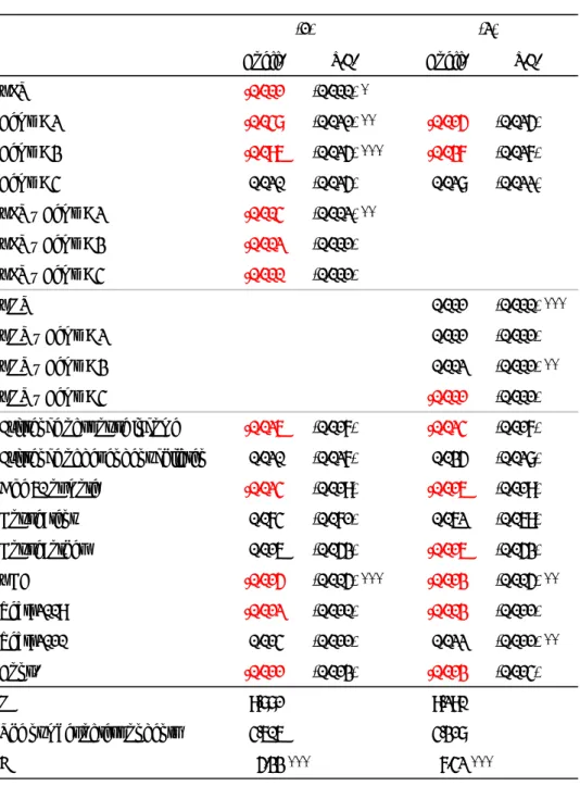
Table 3: Estimated Results from the Fixed Effect Model (Δln C is the response variable)

Note: The numerical value is the regression coefficient and the values between parentheses standard errors. ΔLT is Δ individual resident tax, ΔNT is Δ income tax, and the Cemp variable represents changes in employment status. Cemp = 1 represents maintaining regular employment, Cemp = 2 represents moving from regular to irregular employment, Cemp = 3 represents moving from employment (regular, irregular, or self) to unemployment, and Cemp = 4 represents all other changes. The standard errors are clustered at the respondent level. ***, **, and * represent significance at the 1%, 5%, and 10% levels, respectively.

Coeff. S.E. Coeff. S.E.

ΔLT -0.001 (0.000)^*

Cemp = 2 -0.048 (0.021)^** -0.015 (0.025)

Cemp = 3 -0.096 (0.025)^*** -0.037 (0.027)

Cemp = 4 0.020 (0.025) 0.028 (0.022)

ΔLT × Cemp = 2 -0.004 (0.002)^**

ΔLT × Cemp = 3 -0.002 (0.001)

ΔLT × Cemp = 4 -0.000 (0.001)

ΔNT 0.001 (0.000)^***

ΔNT × Cemp = 2 0.001 (0.001)

ΔNT × Cemp = 3 0.002 (0.001)^**

ΔNT × Cemp = 4 -0.001 (0.001)

Existence of spouse income -0.026 (0.017) -0.024 (0.017) Existence of dependent children 0.020 (0.027) 0.035 (0.028)

Age 60 or more -0.024 (0.019) -0.016 (0.019)

House: rent 0.074 (0.071) 0.062 (0.069)

House: other 0.016 (0.053) -0.016 (0.053)

ΔHC -0.015 (0.005)^*** -0.013 (0.005)^**

Year: 2009 -0.012 (0.010) -0.003 (0.011)

Year: 2010 0.014 (0.011) 0.022 (0.011)^**

Cons. -0.011 (0.013) -0.013 (0.014)

N 9,881 9,290

The number of respondents 4,606 4,318

F 5.33 ^*** 7.42^***

(1) (2)