Residual Ultimate Strength of AxiallyCompressed Tube after Collision or Corrosion

(1)

九州大学学術情報リポジトリ

Kyushu University Institutional Repository

Residual Ultimate Strength of Axially

Compressed Tube after Collision or Corrosion

李, 若轩

http://hdl.handle.net/2324/1959122

出版情報：九州大学, 2018, 博士（工学）, 課程博士バージョン：

権利関係：

(2)

Residual Ultimate Strength of Axially Compressed Tube after

Collision or Corrosion

Ruoxuan Li

Graduate School of Engineering Kyushu University

September 2018

(3)

II

(4)

III

Acknowledgements

First, I would like to express thanks to Japanese government for giving me financial support for the past three-year PhD study and research.

I would like to thank Professor Gu in Shanghai Jiao Tong University who informed me the opportunity to get MEXT scholarship. And I also would like to thank Professor Shinoda who introduced me to Kyushu University.

I would like to express my deepest gratitude to my supervisors Professor Yoshikawa and Professor Yanagihara. I could never have finished this PhD dissertation without their academic guides. I leant a lot about how to conduct perfect research work from them two. In the past three years, my harvest is not only the academic ideas and skills but also the attitude, passion and patience to science and engineering. I would like to say special thanks to dear Professor Yoshikawa, an awesome engineer with rich practical experiences, it was really my honor to work with him and learn from him.

I would like to thank Professor Yasuzawa and Professor Gotoh. They helped me a lot on the lectures. And I also would like to say thanks to Ms. Hamahira from Department of Marine System Engineering Office and Ms. Oiwa from the International Support Office, their supports make the campus life comfortable and convenient. I also want to thank for the help from assistant professor Toh. Thanks to all the doctoral and master students from Laboratory 1 and Laboratory 6, they impressed me very much.

I would like to thank my parents who are always proud of me. Their unconditional love and supports really give me confidence and encourage me to move on.

Finally, I would like to thank my girlfriend Ms. Yidong Tao, her love makes me becoming optimistic and provides great power for me to conquer the difficulties. Her smiles and voice are always like the warm sunshine in winter days.

Ruoxuan Li 31 August 2018

(5)

IV

(6)

V

List of figures

Fig. 1.1 Types of loads acting on a fixed offshore platform ... 3

Fig. 1.2 Inelastic buckling equations and data for axially loaded cylinders plotted by Ziemian et al ^[14] ... 4

Fig. 1.3 The initial imperfection of oval mode by Yudo and Yoshikawa ^[15] ... 6

Fig. 1.4 The relationship between corroded pit diameter and depth observed by Nakai ^[26] ... 8

Fig. 2.1 Modeling of boundary condition at both ends ... 18

Fig. 2.2 Tube and rigid sphere before and after lateral impact in the first stage of the Basic case ... 19

Fig. 2.3 Tube deformation under axial compression in the second stage of the Basic case... 20

Fig. 2.4 Side view of contact area ... 21

Fig. 2.5 Schematic view of deformation ... 21

Fig. 2.6 Time history of axial force of the Basic case ... 22

Fig. 2.7 Impact position offset in y direction ... 24

Fig. 2.8 Impact position offsets in z dirction ... 25

Fig. 2.9 Side view of collision situation of different sphere radius ... 26

Fig. 2.10 Deformation at contact area of the Basic case ... 27

Fig. 2.11 Time history of contact area of the Basic case ... 28

Fig. 2.12 Stress distribution in tube axial direction (σz) and cross section deformation of contact area of Basic case in the first stage ... 29

Fig. 2.13 Relationship between the ratio of ultimate strength of damaged tube to that of intact one and the ratio of total deformation to tube diameter ... 32

Fig. 2.14 Deformed cross section of impact part of the tube of Case T20 T60 ... 34

Fig. 2.15 Deformed cross section of impact part of the tube of Case Basic 0.2, 0.3, 0.4 and Basic case. ... 35

Fig. 2.16 Relationship between calculated residual ultimate strength and proposed parameter λ ... 38

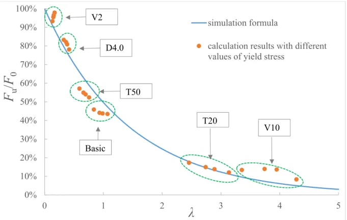
Fig. 2.17 Comparison results between simulated formula and calculation results with different values of yield stress ... 42

Fig. 3.1 Corrosion depth measurement data from Garbatov et al ^[24] ... 48

(11)

X

Fig. 3.2 Corrosion depth measurement data and samples of fitting models from Paik et al ^[46]

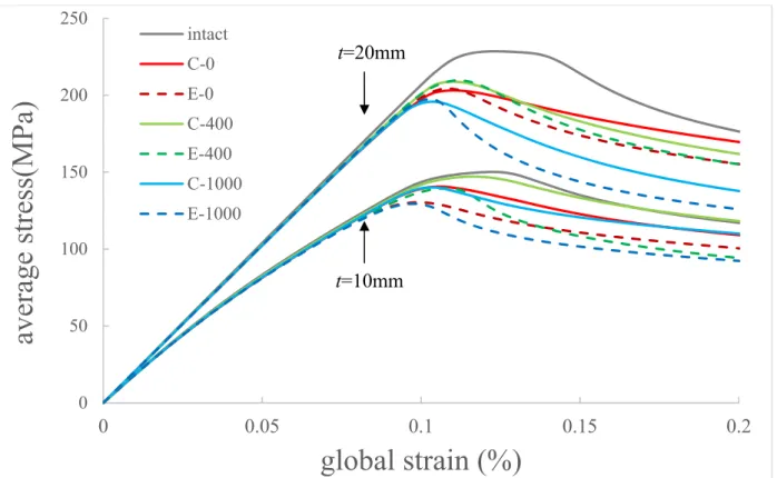
... 48 Fig. 3.3 Calculation model using solid elements for conical pit ... 52 Fig. 3.4 Calculation models using shell elements for circular and rectangular pits ... 53 Fig. 3.5 Assumed thickness distribution for rectangular pit using shell elements (t=20 mm) . 54 Fig. 3.6 Pits positions and plate size of the quarter corroded plate ... 54 Fig. 3.7 Relationship between average stress and global strain of corroded plate with different pit shapes (comparison between solid model and shell model for plate with the size of 800×800mm) ... 56 Fig. 3.8 Relationship between average stress and deflection at plate center of corroded plate (comparison between solid model and shell model for plate with the size of 800×800mm) ... 56 Fig. 3.9 Pit shape: length (l) and depth (d) ... 58 Fig. 3.10 Pit position and numbers for plates with same cross section reduction with different pit shapes ... 59 Fig. 3.11 Relationship between average stress and global strain of corroded plate (comparison between different ratios of pit length to depth with same cross section reduction, t=20mm, w0/t=0.01) ... 60 Fig. 3.12 Relationship between average stress and global strain of corroded plate (comparison between different ratios of pit length to depth with same cross section reduction, t=10mm, w0/t=0.1) ... 60 Fig. 3.13 Simply supported boundary condition ... 61 Fig. 3.14 Detail pit position arrangements of different pit shape with same corroded area size ... 62 Fig. 3.15 Comparison of relationship between average stress and global strain of pit corroded plate of different pit shapes with same corroded area size (t=20mm, w0/t=0) ... 63 Fig. 3.16 Comparison of relationship between average stress and global strain of pit corroded plate of different pit shapes with same corroded area size (t=10mm, w0/t=0) ... 63 Fig. 3.17 Assumed positions of corroded area in plate (t=10mm & 20mm, w0/t=0.1, l=80mm, d=0.5t) ... 65 Fig. 3.18 Relationship between average stress and global strain of corroded plate ... 66 Fig. 3.19 Position of assumed corroded areas (single location of corroded areas or multiple location of corroded areas, t=10mm or 20mm, w0/t=0.1, l=80mm, d=0.5t) ... 68

(12)

XI

Fig. 3.20 Relationship between average stress and global strain of corroded plate (comparison between single location of corroded areas or multiple location of corroded areas, t=10mm or

20mm, w0/t=0.1) ... 68

Fig. 3.21 Corner corroded plates with different ratio of α ... 70

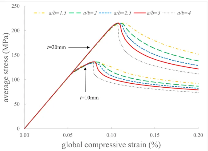
Fig. 3.22 Relationship between average stress and global strain of corroded plate (comparison between different α of plate, w0/t=0) ... 71

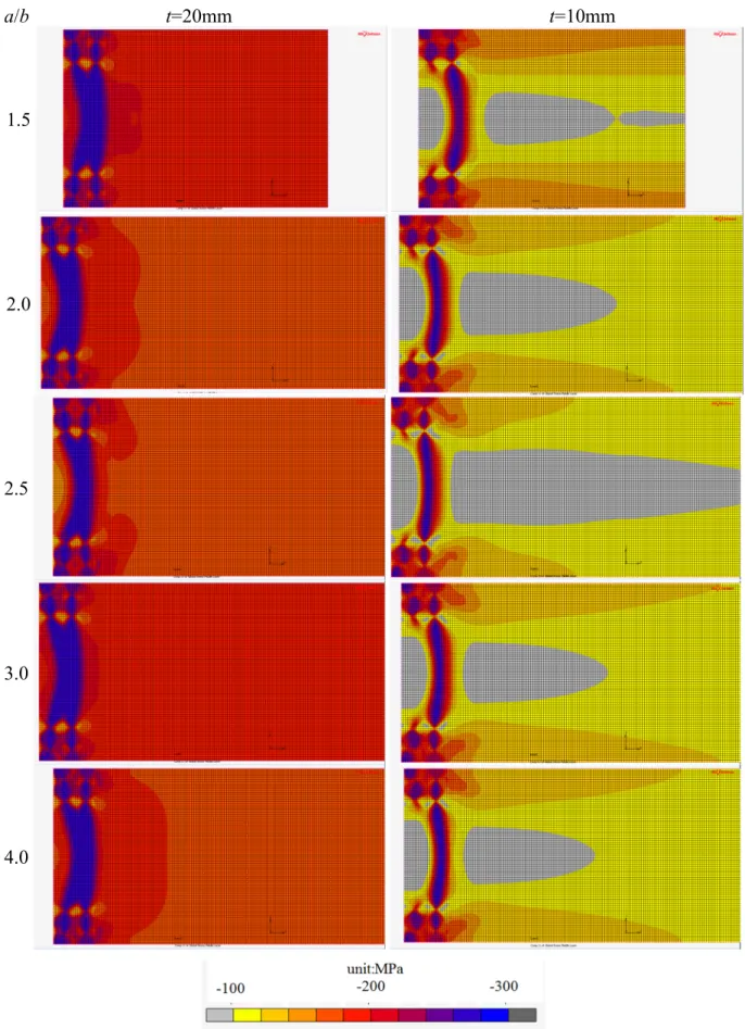
Fig. 3.23 σx distribution of the corroded area at ultimate state of plates with different a/b ratio ... 72

Fig. 3.24 Position of assumed corroded areas (different number of corroded area in length and breadth, t=10mm or 20mm, w0/t=0.1, l=80mm, d=0.5t) ... 73

Fig. 3.25 Relationship between average stress and global strain of corroded plate (comparison between different numbers of corroded area sizes in plate length and breadth directions, t=10 mm or 20mm, w0/t=0.1) ... 74

Fig. 3.26 Different corroded area size in plate breadth direction with the same cross section reduction (l= 80mm, w0/t=0.1) ... 76

Fig. 3.27 Relationship between average stress and global strain of corroded plate (comparison between different corroded area with same cross section reduction, w0/t=0.1) ... 77

Fig. 3.28 Comparison of calculation results and simulated equation ... 81

Fig. 4.1 Simply supported boundary condition ... 85

Fig. 4.2 Corroded area size and position ... 86

Fig. 4.3 Pit arrangement (the shadow parts are pit corroded, the blank parts are intact) ... 87

Fig. 4.4 Comparison of simplified formula and calculation results ... 93

Fig. 4.5 The comparison of calculation results and simulation equation ... 96

Fig. 4.6 Relationship between residual ultimate strength ratio of corroded tubes to intact ones and tube material yield stress ... 99

Fig. 4.7 Calculation results of ultimate strength and computation time of models with different element sizes ... 101

Fig. 4.8 Residual ultimate strength calculation results comparison of corroded tubes with different pit shapes ... 103

Fig. 4.9 Pits arrangement of different pit shapes with the same corroded area size ... 104

Fig. 4.10 Comparison of deformation mode and σz distribution at ultimate state of different pit shape with same corroded area size (factor = 50) ... 105

(13)

XII

Fig. 4.11 Comparison of deformation mode and σz distribution at post ultimate state of different pit shape with same corroded area size ... 106 Fig. 4.12 Comparison of deformation mode and σz distribution at post ultimate state of different pit shape with same corroded area size, ... 107 Fig. 4.13 Pits arrangement ... 108 Fig. 4.14 Comparison of ‘average stress and global compressive strain’ relationship calculation results between l/d=40 and l/d=20 ... 109 Fig. 4.15 Comparison of deformation mode and σz distribution at the ultimate state and post ultimate state ... 110 Fig. 4.16 Comparison of deformation mode and σz distribution at the ultimate state and post ultimate state ... 111 Fig. 4.17 Comparison of deformation mode and σz distribution at the ultimate state and post ultimate state ... 112 Fig. 5.1 Histograms of velocities for general cargo vessels with distributions fitted by Montewka et al ^[56] ... 115 Fig. 5.2 Distribution of ships’ speeds by Silveira et al ^[57] ... 115 Fig. 5.3 Probability density function of tube shell thickness of random series of values (Normal distribution, mean value=40mm, standard derivation=2mm) ... 117 Fig. 5.4 Probability density function of tube material yield stress of random series of values (Log-normal distribution, mean value=269MPa, standard derivation=21.52MPa) ... 118 Fig. 5.5 Probability density function of approaching velocity of random series of values .... 119 Fig. 5.6 Probability density function of impact mass of random series of values ... 119 Fig. 5.7 Calculation result of probability density function of non-dimensional parameter λ of Basic case (mean value of approaching velocity is 3m/s) ... 120 Fig. 5.8 Method to obtain value of vcr ... 121 Fig. 5.9 Calculation result of probability density function of non-dimensional parameter λ of Basic case with the failure possibility less than 0.0013 ... 122 Fig. 5.10 A schematic of the corrosion process for marine structures by Paik ^[46] ... 124 Fig. 5.11 Conceptual model for marine immersion corrosion showing nonlinearity of corrosion behavior with time by Melchers ^[45] ... 125 Fig. 5.12 Method to calculate ΔT based on different corrosion rate models ... 126 Fig. 5.13 Time history of corrosion first appearance ... 128

(14)

XIII

List of tables

Table 1.1 Several noteworthy offshore catastrophes ^{[1, 2]} ... 2

Table 1.2 Stochastic model for geometrical parameters by Gaspar ^[34] ... 9

Table 1.3 Stochastic model for material properties by Gaspar ^[34] ... 9

Table 2.1 Material property of tube members ... 17

Table 2.2 Detail value of parameters in calculation cases ... 23

Table 2.3 Different assemble of impact mass and velocity with same energy ... 25

Table 2.4 Calculation results of deformation, axial force and ultimate strength from parametric study ... 30

Table 2.5 Calculation results of absorbed energy and ultimate strength considering offset effect in y direction ... 33

Table 2.6 Calculation results of absorbed energy and ultimate strength considering offset effect in z direction ... 35

Table 2.7 Calculation results comparison with different impact mass and velocity ... 36

Table 2.8 Calculation results comparison with different shape of impact spheres ... 36

Table 2.9 Comparison of calculation results of different values of shell thickness ... 41

Table 2.10 Comparison of calculation results of different values of Young’s modulus ... 41

Table 2.11 Comparison of calculation results of different values of yield stress (Basic) ... 43

Table 2.12 Comparison of calculation results of different values of yield stress (V2) ... 43

Table 2.13 Comparison of calculation results of different values of yield stress (D40) ... 43

Table 2.14 Comparison of calculation results of different values of yield stress (T50) ... 43

Table 2.15 Comparison of calculation results of different values of yield stress (T20) ... 44

Table 2.16 Comparison of calculation results of different values of yield stress (V10) ... 44

Table 2.17 Comparison of residual ultimate strength between calculation results and allowable axial compressive stress of API rules ^[13] ... 46

Table 3.1 Pit shapes on the corroded plate ... 55

Table 3.2 Calculation cases for the plate of t=20mm with geometrical imperfection w0/t=0.01 (calculation parameter is pit length and depth) ... 58

Table 3.3 Calculation cases for the plate of t=10mm with geometrical imperfection w0/t=0.1 (calculation parameter is pit length and depth) ... 58

(15)

XIV

Table 3.4 Ratios of pit length to depth ... 62

Table 3.5 Results of ultimate strength (comparison of ultimate strength of corroded plate with different positions of corroded area, w0/t=0.1) ... 66

Table 3.6 Results of ultimate strength (comparison of corroded plate with single corroded areas or multiple corroded areas, w0/t=0.1) ... 69

Table 3.7 Plate scantlings details for the effect of ratio of a/b ... 69

Table 3.8 Results of ultimate strength (comparison of corroded plate with different number of corroded area in length and breadth, w0/t=0.1) ... 73

Table 3.9 Residual ulimate stress comparison of corner corroded plate with different level of geometrical initial imperfection (plate size: 2400×800mm) ... 75

Table 3.10 Ultimate strength of corroded plate with different reduction of cross section area (w0/t=0.1) ... 79

Table 3.11 Equivalent reduction of cross section (t=10mm and 15mm) ... 80

Table 4.1 Ultimate strength calculation results of tubes with different corroded area position in axial direction ... 88

Table 4.2 Ultimate strength calculation results of tubes with different corroded area sizes .... 89

Table 4.3 Ultimate strength calculation results of tubes with different cross section reduction ... 90

Table 4.4 Residual ultimate strength of corroded tube with column buckling initial imperfection ... 91

Table 4.5 Residual ultimate strength of corroded tube with diamond buckling initial imperfection ... 91

Table 4.6 Residual ultimate strength of corroded tube with uniform circumferential initial imperfection ... 91

Table 4.7 Ultimate strength calculation results of tubes with different pit depth of additional cases ... 92

Table 4.8 Residual ultimate strength calculation result of tubes with different scantlings. ... 94

Table 4.9 Residual ultimate strength calculation result of tubes with different shell thicknesses (L=30m, D=2.5m) ... 95

Table 4.10 Comparison of calculation results with different values of shell thickness ... 97

Table 4.11 Comparison of calculation results with different values of Young’s modulus ... 98

Table 4.12 Comparison of calculation results with different values of yield stress ... 99

(16)

XV

Table 4.13 Calculation results of ultimate strength with different element sizes ... 102 Table 4.14 Calculation results of ultimate strength of tubes with different level of geometrical initial imperfection ... 102 Table 4.15 Residual ultimate strength ... 109 Table 5.1 Calculation results of upper bound criteria approaching velocity (Mmean=1000ton) ... 123

(17)

XVI

(18)

1

Chapter 1. Introduction

In this chapter, the research background and the organization of this thesis are given. In Section 1.1, a literature review is presented and the gaps in previous research are pointed out. In Section 1.2, the procedures of this thesis are illustrated. In Section 1.3, the organization of this thesis is stated.

1.1 Overview and background

With the transfer of oil and gas industry from land to ocean, the development of offshore structures and related techniques is rapid in recent decades. Among all kinds of offshore structures, the jacket platforms are first applied and used most widely. The followings are the advantages of the jacket platforms.

 The design and manufacture techniques are mature;

 The economical efficiency is outstanding especially in shallow water regions (general below 200m);

 Adaptability for various environment situations;

 The structure stability and safety characteristics is approved.

As the technique of design and manufacture improved and widely explosion in all over the world, the oil and gas production in offshore fields plays an important role in the energy resource supply. Although the leg tubes of jacket platforms are carefully treated from the design stage to the maintenance, accidents still occurred in the past. Several noteworthy offshore accidents summarized by Wang ^[1] and Bhandari et al ^[2] are listed in Table 1.1. Offshore platform is a system of many facilities and complicated procedures, including drilling, storage and transportation and other installations. Hence, if one leg fails, it will cause severe consequence. The damage might only be estimated to be the direct loss. The additional economic losses also contain the fees to repair or replace the broken part of the system, to tear down the offshore structure if the damage is unrepairable defective as well as the costs and efforts to deal with the potential environment pollution caused by the leaked oil.

(19)

2

Table 1.1 Several noteworthy offshore catastrophes ^{[1, 2]}

Accident Year Fatalities Cost due to damage

Umm Said Qatar April 1977 3 died $ 179 million

Ekofish Norway March 1980 123 died

Mexico Pipe Leaking November 198 650 died $ 29 million

Sleipner Norway August 1991 £ 160 million

Piper Alpha North Sea July 1998 167 died $ 1.2 billion Sinking of Erika December 1999 8 died

Roncador Brazil March 2001 2 died $ 515 million

Besides, the negative influences of such accidents also injure the confidence of offshore engineers and restrict the development of offshore techniques. Therefore, to minimize the possibility of accidents is a primary target for both the scholars and practitioners in this field.

The present research focuses on the substructure of jacket platforms which is the supporting construction. Usually a substructure is made up by a series of mild steel tube members by welding. Firstly, the potential loadings of the jacket platforms are shown in Fig. 1.1. As shown in this figure, the main load for the tube members of the substructures are axial loading and bending. The leg tubes are components of the substructure, so the function of leg tubes is to bear the axial compressive load. However, the jacket platform is fixed to the sea bed and it is difficult to move, so the repairing cost is high. Therefore, the residual ultimate strength of damaged tube is worthy to be investigated.

Therefore the central target in the present research is to investigate the axial compressive residual ultimate strength of circular tubes after damaged. The FEM method is applied in this research. With the help of numerical simulation, the residual ultimate strength of tubes is investigated.

There are two kinds of damage, which are introduced into the tube members in this research.

They are accident load and time depending load. As for the accident load, it is described in Handbook of Offshore Engineering ^[3] which includes loads from residual events that may be caused by accidents such as vessel impact, dropped object impact, fire and blast and unusual environmental conditions. Magnitudes of these loads are obtained from a global risk assessment study or based on past experience and code requirements. Platform is generally designed against

(20)

3

these loads with safety factors. And API ^[4] rules are recommended to be referred in the design stage of jacket platforms.

Fig. 1.1 Types of loads acting on a fixed offshore platform

The time depending effect is the corrosion which is a normal phenomenon to be taken into consideration in ship and offshore structures design. Since mild steel is widely used to build constructions, corrosion effect leads to the material loss as time passes. The shell thickness reduction is the main results due to corrosion.

(21)

4

The above mentioned two effects both influence the axial compressive ultimate strength of circular tube members that act as the supporting structures of jacket platforms.

The tube members used in offshore structures as the substructures are in large size ^[5-12]. The scantling range is shown as follows,

Length, L 16~40m;

Diameter, D 2.0~3.5m;

Thickness, t 25~55mm.

And the properties of mild steel will be shown in Table 2.1 in Section 2.2.1.

The critical ultimate strength of the tubes with the D/t less than 100 is almost the yield stress of the material according to Guide to stability design criteria for metal structures ^[14] as shown in Fig. 1.2.

Fig. 1.2 Inelastic buckling equations and data for axially loaded cylinders plotted by Ziemian et al ^[14]

(22)

5

The criteria of judgement on whether the loading capacity of tube members is acceptable or not is according to API rules ^[4]. The allowable axial compressive stress is calculated based on the API rules ^[4] as follows. The API rules ^[4] could provide a reference to determine the residual ultimate strength of damaged tube is acceptable or not.

The allowable axial compressive stress, σa, should be determined from the following formulas.

For tubes with a D/t ratio equal to or less than 60:

2 2

3 3

( / )

1 2

3( / ) ( / )

5 / 3

8 8

y c

a

c c

Kl r C

Kl r Kl r

C C



 

  

 



 

for Kl/r < Cc (1.1-1)

 

2 2

12

23 /

a

E Kl r

   for Kl/r ≥ Cc (1.1-2)

Where,

1

2 2

2

c

y

C  E



 

   ,

σy = yield strength, MPa,

E = Young’s Modulus of elasticity, MPa,

K = effective length factor, Section 3.3.1d, (equals to 1.0 in this research) l = unbraced length, m,

r = radius of gyration, m.

For tubes with a D/t ratio is greater than 60 and less than 300, with wall thickness t>6 mm, both the elastic (σxe) and inelastic local buckling stress (σxc) due to axial compression should be determined from Equation (1.1-3) and Equation (1.1-4). Overall column buckling should be determined by substituting the critical local buckling stress (σxe or σxc, whichever is smaller) for σy in Equation (1.1-1) and in the equation for Cc.

Elastic Local Buckling Stress:

σxe = 2CEt/D (1.1-3) Where, C = critical elastic buckling coefficient (the theoretical value of C is 0.6),

(23)

6 D = outside diameter, m,

t = wall thickness, m.

Inelastic Local Buckling Stress:

 

^1/4

1.64 0.23 / for( / ) 60

xc y xe

xc y

D t D t

  

 

  

    

   (1.1-4)

It is a normal sense that the existence of geometrical initial imperfection leads to the reduction of the ultimate strength of shell structures. Yudo and Yoshikawa ^[15] investigated the effect of initial imperfection on the bending capacity of tubes, in that research the initial imperfection mode is shown in Fig. 1.3.

Fig. 1.3 The initial imperfection of oval mode by Yudo and Yoshikawa ^[15]

Teng at el. ^[16] investigated the behaviors of FRP-circular tubes. And Fraldi and Guarracino ^[17]

tested the geometrical imperfection of cold-formed tubes, and found that n=2 and 3 in Equation (1.2) is the most normal situations. However for the circular tubes under axial compression, the most severe case of initial deflection is uniform symmetrical buckling mode in the circumferential direction and elastic buckling mode in axial direction.

(24)

7

0sin y cos

w w n

L

 

 

   (1.2)

In the field of ship collision with offshore structures, Amdahl ^[18], Hu ^{[19, 20]} and Watan ^[6] all investigated the collision force between ship and offshore structures. However the residual ultimate strength of tube members after such kind of collision has seldom been studied before.

So this important characteristic is studied in this thesis.

The effect of corrosion is a rather complicated phenomenon on ship and offshore structures. In order to avoid the material loss in marine systems, coating is the basic and effective measurement to protect the steel from corrosion. Whereas, the lifetime of coating is limited compared to the lifetime of marine structures. Wang ^[21], Melchers ^{[22, 23]}, Garbatov ^[24] and Paik

[25] measured and investigated corrosion effect on ships with the exposure period. The statistics data of corrosion level and corrosion depth shows that it has a very large variable range. That means the corrosion situation varies very much from one ship to another, from one location of the ship to other locations. It is very difficult to predict the corrosion effect quite accurate in the lifetime of marine structures. So, the maximum pit depth is applied for safety side, generally.

Two types of corrosion are usually considered. One is the general corrosion which is treated as the uniform thickness reduction of the plate and shell. The other is the pit corrosion, this kind of corrosion is more localized. Nakai ^[26] observed the shape of pit corrosion on hold frames of 12, 14 and 20 years-old bulk carriers and a 22 years-old oil tanker. And the relationship between pit diameter and depth is shown in Fig. 1.4. He found that the pit shape is a circular cone and the ratio of the diameter to the depth is in the range between 8 to 1 and 10 to 1 in bulk carriers, and the ratio is in the range between 4 to 1 and 6 to1 in oil tankers. That provide a reference for actual pit shapes.

(25)

8

Fig. 1.4 The relationship between corroded pit diameter and depth observed by Nakai ^[26]

In terms of the modelling of corroded plates in FEM calculation models, the majority of the researches, solid elements of small size are used, such as Ahmmad ^[27]. Shell elements model is also applied, however, pits are arranged symmetrically on both surfaces of the plate, such as Paik et al ^[28] and Wang et al ^[29]. Zhang ^[30] applied shell elements to model the corroded stiffened plate only on one side of the plate. It is assumed that, pitting corrosion almost occurred to overall the plate. It is concluded that the DOP (the degree of pit corrosion intensity defined as the ratio of pitted area to the whole surface area) affected on the ultimate strength of corroded plate. However, the dominant parameter to influence on the residual ultimate strength of pit corroded plate might be the residual cross section area.

The shell thickness geometrical variation and material property is investigated by Shu ^[31], Guedes ^[32], Vhanmane ^[33] and Gaspar ^[34]. The variation ratio of standard deviation to the mean value (design value) of thickness is 5%. That is 8% of material yield stress. And the distribution of thickness and Young’s modulus both obeys normal distribution. For yield stress, the distribution obeys the log-normal distribution. The stochastic model for geometrical parameters and material properties by Gaspar ^[34] is shown in Table 1.2 and Table 1.3, respectively.

(26)

9

Table 1.2 Stochastic model for geometrical parameters by Gaspar ^[34]

Variable Distribution Mean value, μ COV, σ/μ

l (m) Normal Design value 0.05

t (mm) Normal Design value 0.05

cf.) σ is the standard derivation.

Table 1.3 Stochastic model for material properties by Gaspar ^[34]

Variable Material Distribution Mean value, μ COV, σ/μ

σy (N/mm²) Steel, NS Log-Normal 269 0.08

Steel, HS 348 0.06

E (N/mm²) Steel, NS&HS Log-Normal 206000 0.10 cf.) Design values for normal strength steel (NS): σy=235N/mm², 5th percentile;

E=206000 N/mm², mean value.

Design values for high strength steel (HS): σy=315N/mm², 5th percentile;

E=206000 N/mm², mean value.

The physical parameters are not unchangeable values. Every parameter has its own variation range. According to Gaspar et al ^[34], the effects of the variation ranges of tube scantlings, namely length L, diameter D and shell thickness t, and material properties, Young’s modulus E and yield stress σy, are investigated in this thesis.

1.2 The procedures of present research

The purpose of this research is to investigate the residual ultimate strength of damaged tube members. These tube members are used to form the substructures of jacket platforms. The axial compressive loading capacity of tubes is the basic to guarantee of the safety of platforms. Two kinds of damage are mainly discussed here. One is the lateral collision of supply vessels, a dynamic accidental load. The other is pit corrosion, a static time-depending load, since pit corrosion is a more complicated type than general corrosion which is treated to be the reduction of thickness.

(27)

10

In the research of collision effect on tube residual ultimate strength, numerical simulation is performed applying LS-Dyna, which is a non-linear FEM software widely adapted in collision and explosion. The residual ultimate strength of damaged tubes is calculated. Referring the API rules, the acceptable value of the residual ultimate strength of damaged tubes is determined.

In the research of corrosion effect on tube residual ultimate strength, MSC.Marc is applied to calculate static calculations. MSC.Marc is applied for static analysis. The method to model the corroded area of plate structure with shell elements is investigated. This method shall provide accurate results and time efficient. By applying this method, the residual ultimate strength of corroded tubes is studied using large size of shell elements.

To assess the safety of damaged tubes in the design and maintenance, it is required to easily predict the residual ultimate strength. Simplified formulae are also derived to predict the residual ultimate strength considering the FEA results.

The probability study on the collision effect is also required to be performed, considering the variation of material yield stress and shell thickness. The colliding mass and velocity variations are important factors in collision effect research. In corrosion effect, the timespan between two inspections based on the predictions of the strength reduction and corrosion depth is investigated.

1.3 Organization of present thesis

In Chapter 2, the residual ultimate strength of tube members after lateral impact is studied. A series of numerical simulation is performed in LS-Dyna. Parametric study is accomplished by changing the tube scantling and impact energy. Also the effect of impact shape and impact position are also investigated. Based on the residual ultimate calculation results. The parameter, λ, is proposed to represent the relative anti-impact ability of tubes. A non-dimension formula is derived to describe the relationship between residual ultimate strength of damaged tube and this parameter. Then the API rules are referred to estimate the critical acceptable damaged situation.

Final, the effect of variable material physical properties is investigated.

(28)

11

In Chapter 3, the residual ultimate strength of pit corroded plates is studied as a preliminary step for investigation of the residual ultimate strength of pit corroded tubes. Numerical simulations are performed by MSC.Marc. Firstly, a method is proposed to model corroded area of shell structures with shell elements. It is proved that this method is time efficient with reasonable accuracy. Secondly, the residual ultimate strength of pit corroded plate is investigated by applying the above method. A typical size of the plates used in marine structures is adapted. The crucial parameter to influence on the residual ultimate strength of pit corroded plate is examined. A formula is derived to describe the residual ultimate strength of corroded plate.

In Chapter 4, the residual ultimate strength of pit corroded tube is investigated. Tube scantling parameter study is performed. The relationship between the residual ultimate strength of pit corroded tube and the corrosion level is obtained. Moreover, the effect of variable material physical properties is investigated as well.

In Chapter 5, the engineering suggestions are carried out. For the collision effect on tubes, probability of failure of collided damaged tubes is investigated. With the application of the simplified formula proposed in Chapter 2, Monte Carle method is used to point out the safety criteria value of impact energy. Base on that, a suggestion of the approaching velocity of supply vessels is proposed. For the corrosion effect on tube members, the relationship between residual ultimate strength and corrosion rate is investigated with the help of the simplified formula proposed in Chapter 4. Thereby, the approach of maintenance is suggested.

In Chapter 6, the researches of present paper are summarized and concluded. And future works are discussed.

(29)

12

(30)

13

Chapter 2. Residual Ultimate Strength of Circular Tube after Lateral Collision

2.1 Introduction

Circular steel tubes have been widely applied as the basic element of substructure of fixed offshore structures, such as jacket platforms. The main function of supporting tube is to bear axial loading, especially axial compressive load. As a fixed offshore structure, jacket platforms may suffer from many kinds of accidental load, for example, the lateral impact by supply vessel and floating objects. These accidents will influence the load capacity of supporting tube. Such kind of impact will lead to plastic deformation on tube members. As a result, the ultimate strength of tubes will decrease compared to that of intact ones.

This chapter focuses on the assessment of ultimate strength of the tube structure after collision impact. Ship collision is a dynamic phenomenon with high energy. Minorsky ^[35] first summarized 26 events, and provided formulae describing the relationship between the damage volume and energy dissipation. This method had been widely used in this area by many researchers.

Amdahl ^[18] and Wierzbicki and Suh ^[36] both investigated the deformation model of circular tubes under lateral impact. However, the lateral load in Amdahl’s research was applied by a rigid plate parallel to the tube axis. While the load in Wierzbicki and Suh’s ^[36] research was applied by a line impact onto one section of the tube. Then they derived the relationship of lateral deformation of the tube and energy dissipated in collision. But the above scenario that a supply vessel impacts laterally to the supporting tube of jacket platforms is not the most dangerous of collision cases. In the other hand, it seems to be more dangerous that the bow structure collides to the tube members. Nevertheless, this kind of collision cases have not been investigated by them.

(31)

14

Based on Amdahl and Wierzbicki and Suh researches, Hu ^{[19, 20]} investigated the relationship between colliding force and indentation using analytical, numerical and experimental methods.

However, the residual ultimate strength after collision was not investigated.

Other works ^[37-39] focused on the failure mode of the tubes under axial compression, and in those researches the tubes were relatively short ones, with the L/D ratio around 1~10.

Meanwhile the L/D ratio for jacket platforms is larger than that, about 40. Where L and D is the length and diameter of the tube member.

Watan ^[6] investigated the collision between the side structure of supply vessel and the jacket platform tube. In his work, collision velocity, collision position along the tube axis and tube geometric parameter have been varied. Finally, the relationship among the collision force, energy and impact indentation have been derived. The scenario of the collision between jacket platforms and supply vessels is bow impact. He concentrated on the collision force rather than the ultimate strength of the tube after collision. In his FEM model, the tube thicknesses were 30, 40 and 50mm, the element length was 100mm, and the ratio of element length to thickness was 2~3.3.

The shape of ship bow has been illustrated by several researchers based on real ship structures.

Shown by Storheim and Amdahl ^[7], the actual collision is within 11~14MJ range, directed by NORSOK rules. The bulbous radius along the centerline was approximately 2m and 1m along the stringer deck in the middle of the bulbous.

In Travanca and Hao ^[8]research, the height of this vessel is 6.3m and deadweight is 3000ton.

The diameter of bulbous bow is about 2m. And the tube length is ranging about 25m, with diameters of 1.28-1.70m.

Yu and Amdahl ^[5] also analyzed the tubular members of offshore structures impacted by ships.

The length, diameter and thickness is around 20m, 1.5m and varying from 30 to 50mm. The bulbous diameter is approximately 2.0m.

(32)

15

Bela et al ^[9] investigated the collision between the Offshore Wind Turbine and Offshore Supply Vessel. The yield stress of the material for the circular column structure of Offshore Wind Turbine was around 250MPa. The vessels were 3000 and 5000ton of DWT. Collision velocity range was from 1 to 5m/s. In his calculation results, after the impact of ship with the velocity of 5m/s, the tube had almost lost the bearing capacity under the axial load.

And then Bela et al ^[9] performed additional numerical simulation to investigate the energy dissipation of the above scenarios with deformable striking ship model. With the high collision velocity about 5m/s, the offshore structure absorbed up to 80% of the total energy.

Most of previous researches focused on predicting the collision force, the interaction with ship structure and the energy dissipation. They concerned more about the collision event itself. In the present study, the main objective is the residual load carrying capacity of the offshore tubes after impact. In this chapter, the ultimate strength of damaged circular tubes in axial direction was investigated. The residual axial ultimate strength of damaged tube after collision was mainly discussed. That was compared to the ultimate strength of intact tubes.

In order to make a decision on whether to repair or replace the members or not, it is crucial to know the residual strength of the tubes. After being damaged by lateral impact, the simply supported tubes will definitely loss a certain extent of load carrying capacity under uniform axial compression.

Therefore, in this chapter, the relationship between the residual ultimate strength of the damaged circular tube by collision and the energy dissipation due to lateral impact is investigated. The influences of several parameters, such as the length, diameter and thickness of the tube and the impact energy, on the reduction of ultimate strength are investigated.

A series of calculations by changing the scantling of tube and colliding conditions is first undertaken to obtain the reduction rate of the residual ultimate strength of damaged tube to that of intact one. In these calculations, the location of damage was assumed to be at the middle span of the tube. Secondly, a simplified formula was derived to predict the residual ultimate strength of the circular tube. And then, by changing the collision position, the applicability of the

(33)

16

proposed formula was examined. By comparing with the allowable compressive stress proposed in API rules ^[4], the critical damage of tube due to collision impact to be repaired is proposed.

Finally, the applicability of proposed formula is investigated by considering the variation range of tube thickness and material properties.

2.2 Basic Case

The purpose of this chapter is to investigate the residual ultimate strength of the tubes that collided and deformed. Firstly, the nonlinear FEM analysis was performed to investigate the residual deformation that was caused by collision. Next, the residual ultimate strength of the deformed tube under axial compressive force was examined. All numerical calculations in this chapter were computed utilizing the nonlinear FEM software LS-DYNA, which is widely used in the research field of ship collision and very good accuracy is approved by many previous researchers, such as Watan ^[6], Yu and Amdahl ^[5] and Bela et al ^[9]. The calculation model and calculation method will be shown below.

2.2.1 Dimension and material of tube

The dimensions of tubes are chosen according to actual size of ship and structure referring the study of Watan ^[6], Travanca and Hao ^[8]and Yu and Amdahl ^[5]. The length, diameter and thickness of legs used in jackets substructures in their studies are in the range of 16~40m, 2.0~3.5m and 25~55mm respectively.

So the Basic case of this chapter was decided as that the length (L), diameter (D) and thickness (t) of the tube is 30m, 2.5m and 40mm, respectively. And the impact mass (M) is 1000ton with the initial velocity (V0) of 5m/s.

The material properties of the tubes are shown in Table 2.1, where the mild steel with the σY=235MPa was selected because of the wide application of this kind of steel in offshore structures.

(34)

17

Table 2.1 Material property of tube members

Items Parameters

Yield stress 235MPa

Mass density 7850kg/m³

Young’s modulus 2.1×10⁵MPa

Poisson’s ratio 0.3

Strain rate parameter, C 40.4 s^{-1 [13]}

Strain rate parameter, P 5.0 ^[13]

cf.) C and P are the parameters in Cowper-Symonds equation:

1

1 ^P

d

s C

 



    

 ;

σd and σs are the dynamic and static stress, respectively.

2.2.2 Striking load

As stated in introduction, up to 80% of the total impact energy was absorbed by the collided offshore structure in collision of ship. The bow structure is stronger than the side part of the supply vessel. And the stiffeners are much more concentrated in the bulbous bow than the upper structure. For most ship the extending distance of bulbous bow is almost the same as the upper structure. As a results, the most severe situation is that the tube members is struck by the ship bulbous bow. From a conservative point of view, the colliding object was assumed to be rigid.

Based on the real structures applied in previous researches Storheim and Amdahl ^[7], Trtavance and Hao ^[8], Yu and Amdahl ^[5] and Bela et al ^[9], a sphere with the diameter of 2.0m is applied as the colliding body in this chapter.

Although the cruising speed of supply vessel is about 15~20knot, the velocity could slow down below 10 knot when collision might occur. Then, the impact velocity of 5m/s (about 10knot) is selected as Basic case. Large deadweight of striking vessel leads to severe deformation to the tubes, such as Bela et al ^[9] stated. Because the residual ultimate strength of damaged tube cannot be expected in such large amount of impact energy cases, these cases are excluded in this chapter. In order to avoid the extreme situations, the impact mass was selected to be around 1000ton.

(35)

18

2.2.3 Boundary condition

For a tube used as jacket leg, other leg tube and brace tube are connected to it on both ends. The bending rigidity of brace members is much smaller at that of leg tube. Therefore at the ends of a tube, the rotation displacements can easily occur. On the other hand the translated displacements are almost constrained. Then, the simply supported conditions were selected to be the boundary conditions at both end of tube as shown in Fig. 2.1. In order to apply the simply supported conditions at both ends of tube, all nodes at each end of tube were connected to the center point of each end section with rigid elements, and the displacements in x and y directions were constrained at both center points. Both cross sections of tube ends were assumed not to deform during the whole process, since neither the collision nor the compression would not influence on the deformation of both ends cross section.

Fig. 2.1 Modeling of boundary condition at both ends

2.2.4 Meshing division

The tube was divided into 100 elements in the circumferential direction with the four nodes Belytschko-Tsay ^[42] shell element, and the sizes of elements in tube circumferential and axial directions are closed to each other. The element size is 78.5×78.5mm for the Basic case, and the ratio of element length to thickness was nearly 2.0 as the thickness of tube is 40mm. In order to verify the validity of this element size, a case with smaller element size of 40×40mm is calculated. Almost the same results are obtained.

Center of tube at end section

At the center points of both tube end, the displacements in x and y directions are constrained All nodes at each end of tube are connected to the center point of each end section with rigid elements.

y x

(36)

19

2.2.5 Loading procedure

There are two loading stages in the simulations in this chapter. The first stage is the lateral impact by a rigid body to the tube at the mid span of the tube, and the second stage is the axial compression of the tube. Then, the calculation time of first stage is set to 0~5.0s, and that of second stage is set to 5.0 ~12.0s.

The initial configuration of tube before lateral impact and the deformation after impact are shown in Fig. 2.2. The circular ones in the figures show the colliding rigid body. The rigid body has an initial velocity of 5.0m/s and a mass of 1000ton in the Basic case. The ends of the deformed tube rotated freely after collision.

Fig. 2.2 Tube and rigid sphere before and after lateral impact in the first stage of the Basic case

The typical deformations of tube under axial compression in the second stage are shown in Fig.

2.3. In this case the center point of left side is fixed in z direction while the that of right side is moving towards left with the velocity of 0.02m/s (the length of the tube is 30m). When the tube suffers the axial compression, the cross section at the middle span of the tube will deform in the same direction as well as the residual plastic deformation caused by lateral impact.⁺

t=0s

t=0.64

(37)

20

Fig. 2.3 Tube deformation under axial compression in the second stage of the Basic case In addition, the above velocity of 0.02m/s was confirmed to be sufficiently low speed to represent the quasi-static behavior of axially compressed tube by the parametric calculation of changing velocity.

2.2.5.1 Calculation of residual deformation in collision

Fig. 2.4 shows the side view of contact area between the collided tube and the colliding sphere.

In this figure, the center of contact area is the front point of the tube. The deformation in the vicinity of the front point is separated into two modes. One is the global deformation of tube as a column. The other is the local deformation at contact section. In this chapter, the separation of these two deformations is estimated from the numerical results.

Since the tube is simply supported at both ends, and the collision position is the middle span of the tube, the section of both ends will share a unique angle of rotation θy while the tube is impacted by the rigid sphere as shown in Fig. 2.5. Then, the global displacement δg can be evaluated by multiplying this rotational angle to the half of tube length, that is δg=1/2L×tanθy. Where, L is the length of tube. The displacement of front point consists of global deformation and local deformation. Then, when δt is defined as the total displacement of the front point, local displacement δl could be calculated as δt ‒ δg. The results will be shown later in Section3.1.1. The time history of reaction force FB at bottom end during the first stage is shown later, in Fig. 2.6.

t=6s

t=10s

(38)

21

Fig. 2.4 Side view of contact area

(a) Overall deformation of tube (b) Cross sectional deformation at contact point Fig. 2.5 Schematic view of deformation

Front point

δt

δg

θy

(39)

22

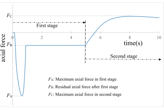
Fig. 2.6 Time history of axial force of the Basic case

2.2.5.2 Calculation of residual ultimate strength of tube under axial compression

At the second stage, the enforced displacement at the center of one tube end was imposed by a constant compressive velocity of 0.02m/s in the tube axial direction, meanwhile the other end was fixed in axial direction. The maximum value of axial force FC shown in Fig. 2.6 will represent the bearing capacity of damaged tube. The difference value between FC and FB can be regarded as the residual ultimate strength of damaged tube, which was struck by lateral impact.

2.3 Effects of collision factors

In order to obtain a simplified formula for prediction of the residual ultimate strength of the damaged tube, a comprehensive parametric analysis is undertaken. The effects of various factors are studied, including the scantling parameter of the tube, the mass, velocity and size of the colliding body, and the collision location. Then the effect of different shapes of striking body is investigated, as well as a detailed analysis by considering various assembles of mass and velocity at the same collision energy.

0 2 4 6 8 10

axial force

time(s)

FA: Maximum axial force in first stage FB: Residual axial force after first stage FC: Maximum axial force in second stage FC

FA

FB

First stage

Second stage

(40)

23

2.3.1 Parametric study of shape of tube and collision energy

The combinations of parameters selected in calculations are shown in Table 2.2. In all cases a rigid sphere with the diameter of 2.0m is modeled as the colliding object.

Table 2.2 Detail value of parameters in calculation cases

Case L (m) D (m) t (m) M (ton) V0 (m/s)

Basic 30 2.5 0.04 1000 5

L15 15 2.5 0.04 1000 5

L24 24 2.5 0.04 1000 5

L38 38 2.5 0.04 1000 5

L45 45 2.5 0.04 1000 5

D1.8 30 1.8 0.04 1000 5

D2.0 30 2.0 0.04 1000 5

D3.2 30 3.2 0.04 1000 5

D4.0 30 4.0 0.04 1000 5

T20 30 2.5 0.02 1000 5

T30 30 2.5 0.03 1000 5

T50 30 2.5 0.05 1000 5

T60 30 2.5 0.06 1000 5

M5 30 2.5 0.04 500 5

M8 30 2.5 0.04 800 5

M15 30 2.5 0.04 1500 5

M25 30 2.5 0.04 2500 5

V2 30 2.5 0.04 1000 2

V3 30 2.5 0.04 1000 3

V7 30 2.5 0.04 1000 7

V10 30 2.5 0.04 1000 10

cf.) L, D and t are the length, diameter and thickness of the tube member, respectively;

M is the mass of rigid impact sphere;

V0 is the initial velocity of the rigid impact sphere before collision.

Colliding position is the center of middle span of the tube. Simply supported condition at both ends of tube is applied in all cases, just as the Basic case. By changing the scantling of the tubes

(41)

24

and the impact mass and velocity, a series of calculations is performed to investigate the parametric effect on the residual ultimate strength of damaged tubes.

2.3.2 Effect of offset in y direction (transverse location)

In the calculation of offset effect both in y direction and in z direction, not all the cases shown in Table 2.2 are calculated. Only these cases were calculated, Basic, L15, L45, D1.8, D4.0, T20, T60, M5, M25, V2 and V10.

Fig. 2.7 shows the definition of the offset of colliding position in y direction. By changing the impact angle α from 0˚ to 60˚, the offset effect in y direction is investigated.

2.3.3 Effect of offset in z direction (longitudinal location)

In order to investigate the effect of colliding location in length on the residual deformation, four cases were performed and compared to each other. Fig. 2.8 shows the detail of colliding position for each calculation case. Where, the length of 3m is 10% of the tube length.

Fig. 2.7 Impact position offset in y direction

(42)

25

Fig. 2.8 Impact position offsets in z dirction

2.3.4 Different assembles of impact mass and velocity

Impact energy is given by the product of the impact mass and the square of velocity. In order to confirm that only the impact energy will influence on the residual ultimate strength of tube rather than the mass or velocity, five cases shown in Table 2.3 were calculated. And Case

*1000-5 is the Basic case of this chapter. In all five cases, the tube scantling was the same as that in the Basic case. The change of impact mass was realized by changing the density of the impact rigid sphere.

Table 2.3 Different assemble of impact mass and velocity with same energy

Case M (ton) v0 (m/s)

*25000-1 25000 1

*6250-2 6250 2

*1000-5 (Basic) 1000 5

*391-8 391 8

*250-10 250 10

2.3.5 Different sizes of colliding object

In order to examine the effect of different geometrical sizes of colliding objects, the calculations of colliding and residual ultimate strength were performed for three different radius (r), 0.3, 1.0 and 3.0m, of the rigid sphere body. Tubes’ scantling was the same as the basic one. The lateral impact mass in all cases is 1000ton with the same initial impact velocity of 5m/s. In this section, r=1.0m is the Basic case of this chapter. Fig. 2.9 shows the deformation of tube in collision, in which the tube and impact sphere was cut by plane in XOZ through the tube axis.

0.2 0.3

0.4 0.5