九州大学学術情報リポジトリ
Kyushu University Institutional Repository
レイリー・ベナール系でのカオス的移流による異常 拡散と混合
大内, 克哉
Graduate School of Sciences, Kyushu University
https://doi.org/10.11501/3075381
出版情報:Kyushu University, 1993, 博士(理学), 課程博士
Anomalous Diffusion and Mixing of Chaotic Advection in a Rayleigh-Benard Flow
Katsuya OUCHI
Department of Physics
J(
yushu University 33,Fukuoka
812March 1993
Contents
1 Introduction
2 Review of Dynamical Systems 2.1 Poincare map . . . . 2.2 Fixed points and their stability 2.3 Invariant manifolds
2.4 Pips and lobes . . .
2.5 Dissipative and conservative systems
1
12 12 14 16 19 25
3 An Experiment on Diffusion by Solomon and Gollub 28 3.1 Diffusion of tracer particles in Rayleigh-Benard convection 28 3.2 Elucidation in terms of Lagrangian turbulence . . . 30
4 Some Characteristics of Diffusion Constant 34
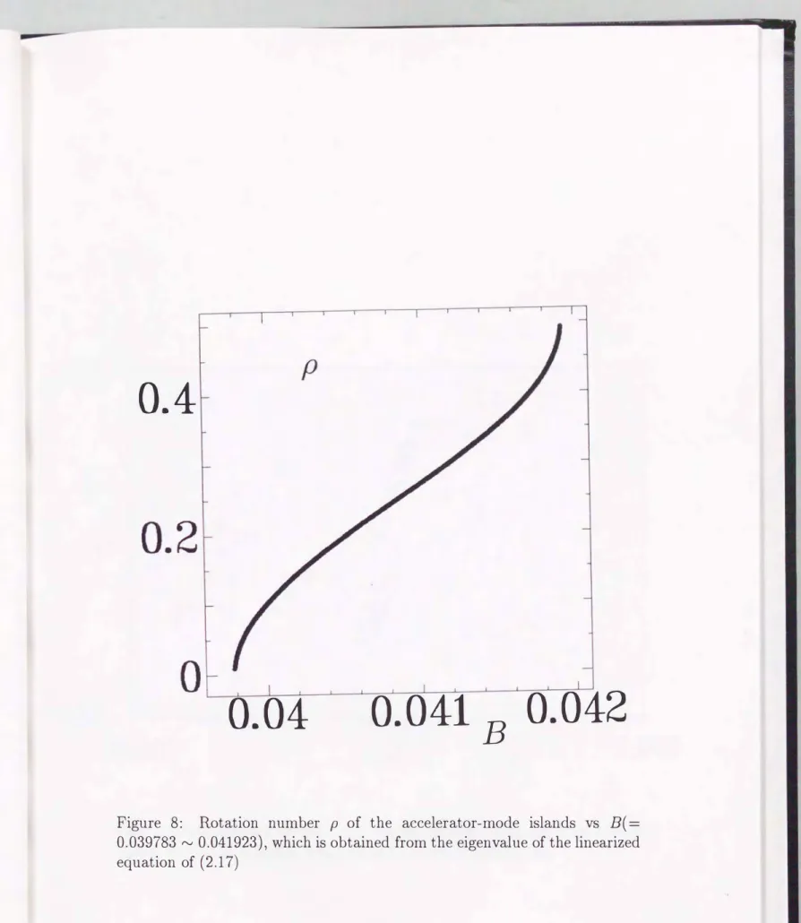
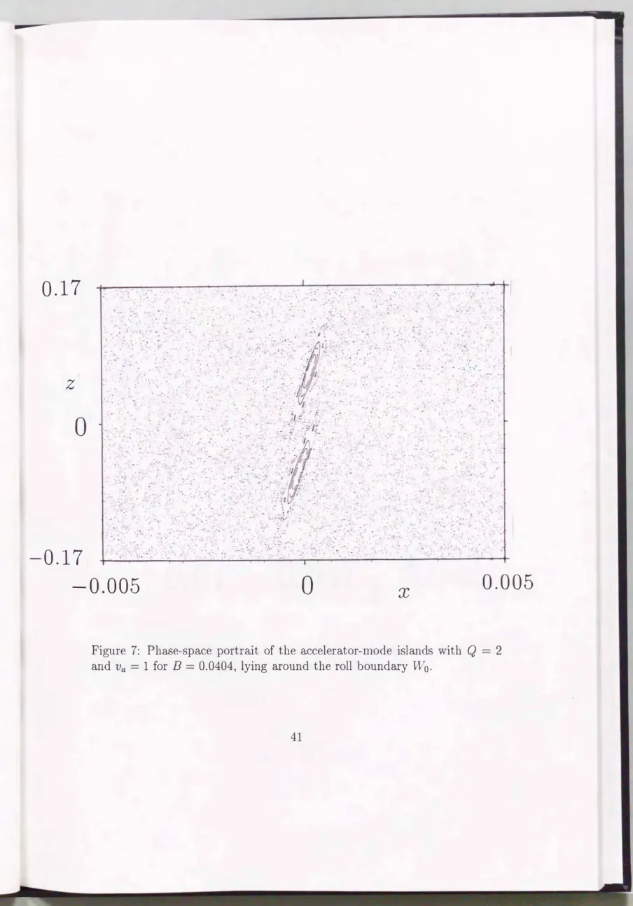
5 Accelerator-mode Islands 40
5.1 Existence of accelerator-mode islands 40
5.2 Long-time correlations of particle orbits 47
6 Diffusion and Accelerator-mode Islands in terms of the Lobes 51
6.1 Lobes and turnstiles in Rayleigh-Benard convection . . . . . 51 6.2 Elucidation of enhanced diffusion and accelerator-mode is-
lands . . . . . . . . 54
�--�---��
6.3 Long-time correlation due to accelerator-mode islands . . . . 59
7 Distribution of Coarse-grained Expansion Rates and its Anoma
lous Scaling 63
8 Summary Acknowledgments Appendix A
70 73 74
Abstract
Solomon and Gollub discussed a transport property of fluid particles in nearly two-dimensional, time-periodic Rayleigh-Benard convection. They deter
mined the diffusion constant D in tern1s of Fick's law by taking only short time characteristics of the trajectories. In this thesis D is defined by the vari
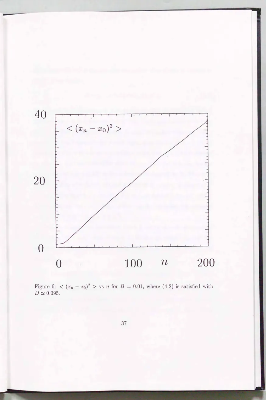
ance for large time. Hence D is determined by the long time correlation of the trajectories, and several fine-grained peaks are observed in the graph of D vs the amplitude B of lateral oscillation. Accelerator-mode islands appear around the oscillating roll boundaries in a peak range of Band the formation of the islands are elucidated in terms of the lobe dynamics.
Mixing of tracer particles by chaotic advection is discussed in terms of the spectrum
1/J(A)
and the probability densityP(A; n)
of the coarse-grained expansion ratesAn.
These physical quantities show an anomalous scaling due to the intermittent sticking of tracer particles to the islands.1/J( A)
has a linear part of slope 0, i.e.,1/J(A)
== 0 for 0<A< A00,
whereA00
is the Liapunov exponent.P(A; n)
obeys an anomalous scaling lawP(A; n)
=n8p{n8(A
A00)}
with 8< 1/2,
wherep(x)
is a power law function for-x
>>1.
These characteristics are generic in Hamiltonian dynamical systems.1 Introduction
The study of chaotic motions in nonlinear oscillator systems has been one of rapidly growing fields of physics for the last decades, with applications to a number of areas in science and engineering, including astronomy, plasn1a physics, statistical mechanics and hydrodynamics. Although the root of the fields is old, dating back to the last century when Poincare and others at
tempted to formulate a theory for nonlinear perturbations of planetary orbits
[
1]
, the field progressed remarkably in the 1960's, together with computational results obtained by using high speed computers, that facilitated our new treatment of the subject. The systems, however, had been mainly con
cerned with conservative ones. Further in the 1970's, an another field of the chaotic properties, i.e., dissipative systems, began to progress with the dis
covery of strange attractors. A strange attractor was found numerically in 1963 by Lorentz
(2],
and the idea was elavorated mathematically in 1971 by Ruelle and Takens[
3]
as a key element in understanding irregular behavior described by deterministic equations, notably turbulence.A main emphasis in both systems is the existence of sequential stretch
ing and folding processes, which lead to the intrinsic stochasticity in the deterministic system. The processes are very important since they mediate between stochasticity and determinism. For example, when the motion of tracer particles in the Rayleigh-Benard convection is studied below, it can be regarded as a diffusion process in spite of the fact that the equation of motion is deterministic. Such the processes lead to a mixing of particles, and
hence the mixing is one of the main themes in studying the chaotic motions.
It is often useful to regard the motion of tracer particles in hydrodynamic flows as a conservative motion. The particle is considered as a virtual particle;
namely a particle with proper mass which does not affect the velocity field and which is not stirred due to the Brownian effect. The motion is determined from a velocity field
v( r, t)
withdrfdt
==v(r, t) (1.1)
and is denoted as the Lagrangian representation. The kinetic equation to determine the velocity field
v( r, t)
is the Navier-Stokes equation, which is a well-known nonlinear partial-differential equation. Hence the behavior of the tracer particles is easily analyzed both theoretically and experimentally.The control parameter of the equation is the Reynolds number formed from the three parameters, the velocity of the main stream, one linear dimen
sion and the kinematic viscosity
[5].
For sufficiently large Reynolds number, the velocity field is turbulent temporally and spatially, and the state is sometimes referred to as the Eulerian turbulence. The tracer particles are of course chaotic in that regime. The turbulence has been studied for a long time and much have been obtained.
Aref, on the other hand, first showed in
1984
that the tracer particles may be chaotic even in laminar flows[6],
where the regime is referred to as the Lagrangian turbulence as compared with the Eulerian turbulence. The viewpoint is as follows. For two-dimensional incompressible flow, the equation for tracer particles
( 1.1)
is formally a Hamiltonian equation with justone degree of freedom. For unsteady flow, the system is non-autonomous and one must in general expect to observe chaotic particle motion. He devel
oped these ideas and subseqently corroborated through the study of a very simple model which provides an idealization of a stirred tank. In the model the fluid is assumed incompressible and invicid, and its motion wholly two
dimensional. the agitator is modeled as a point vortex, which, together with its image in the bounding contour, provides a source of potential flow. The motion of a tracer particles in this model device is cornputed numerically. It is shown that the deciding factor for integrable or chaotic particle motion is the nature of the motion of the agitator. With the agitator held at a fixed position, integrable tracer particle motion ensures, and the model device does not stir very efficiently. If, on the other hand, the agitator is moved in such a way that the potential flow is unsteady, chaotic tracer particle motion can be produced. This leads to an efficient stirring.
These ideas are quite generic for incompressible hydrodynamical flows, and hence many other fluid systems have been studied after Aref's first work.
For example, D.S.Broomhead and S.C.Ryrie studied the trajectories of indi
vidual tracer particle moving in velocity fields which model Taylor vortices close to the onset of the wavy instability
[7).
In particular, they consider the possibility of transporting particles between rolling cells. By studying the flow in the context of dynamical systems theory, it is shown that this arises through the destruction of invariant surfaces which form the roll boundaries in the absence of the wave. Particles able to pass between cells follow chaotictrajectories.
An important characteristic in studying the Lagrangian turbulence is that chaotic structures can be easily analyzed both theoretically and experimen
tally. Indeed, Franjione, Leong and Ottino showed experimentally that sim
ple two-dimensional time-periodic flows produce chaotic mixing and, depend
ing on the choice of the period, large dynamical structures called islands, that change the form in a time-periodic manner but remain segregated even after long times
[8).
Since an analytic expression for the velocity field does not exist in this system, making theoretical prediction of the location and size of islands is impossible. Hence the flow is analyzed in terms of its symmetries which is obtained from the gross properties of the velocity field. With this knowledge, an island is moved into a region of good mixing in a systematic way by manipulating symmetries.Ishii, Iwatsu, Kambe and Matsumoto studied a three-dimensional flow of viscous incompressible fluid in a cubic space with a moving upper wall by solving numerically the N avier-Stokes equation itself
[9).
Steady solutions are obtained at low Reynolds numbers. It is found that the trajectories of the tracer particles exhibit complicated structures even in the steady-state flow fields. The characteristics of the trajectories are examined in detail for a wide range of the Reynolds number. At the low Reynolds numbers in the steady regime, some sets of helical trajectories form invariant tori.As the Reynolds number increases in the region, certain invariant tori are disrupted by resonances and a region of chaotic trajectories coexists with
... ____
regions of invariant surfaces. The chaotic region becon1es larger in the space at higher Reynolds numbers. They ensured that the particle motion in a steady solenoidal velocity field is equivalent to a non-autonomous Hamilto
nian system of one-degree-of-freedom.
In general, an onset of the Lagrangian turbulence is related to a bifurca
tion of the velocity field, but the onset is generally not related to the onset of the Eulerian turbulence. The former is usually lower than the latter. M. Fal
cioni, G. Paladin and A. Vulpiani discussed the connection of this Lagrangian turbulence with behaviors of the velocity field
[10]
both in the Lorentz model[2)
and in truncated N avier-Stokes equations. They indicate a possible road for the onset of Lagrangian turbulence which seems to be rather generic. It is found that the Lagrangian turbulence appears when the velocity field passes from a steady state to a periodic one via Hopf bifurcation. It is also shown that the transition to Eulerian turbulence does not affect the properties of particle motion as noted above. They further discussed an atypical example where it does not exhibit the Lagrangian turbulence even when it is chaotic in the Eulerian sense.The transport properties of two-dimensional incompressible flow between adjacent convection rolls in the temporally oscillating Rayleigh-Benard con
vection with a large aspect ratio were discussed by Solomon and Gollub both experimentally and theoretically
[20].
The contents will be reviewed in § 3 in detail. The Rayleigh-Benard convection is a hydrodynamic flow between horizontal layers heated from below. The fluid, in the incompressible case, isgoverned by the hydrodynamic equations
[5]
Pr-1(av;at +
(v .v)
v) = -Vp + fe + V
2v,ae ;at+
v.VB = Rk.
v +V
2B
,v
·v=O '(1.2)
with two nondimensional control parameters: the Rayleigh number
R
and the Prandtl numberPr.
Here v denotes the velocity field,p
the pressure,B
the temperature difference from the elemental temperature distribution, and
k
the unit vector in the vertical direction. Any flow type of the velocity field v is determined with a pair of the parameters,R, Pr,
and the wave numbera. When the Rayleigh number
R
increases, a time-independent laminar flow with a ==3.117
appears atR
==Rc(
==1707).
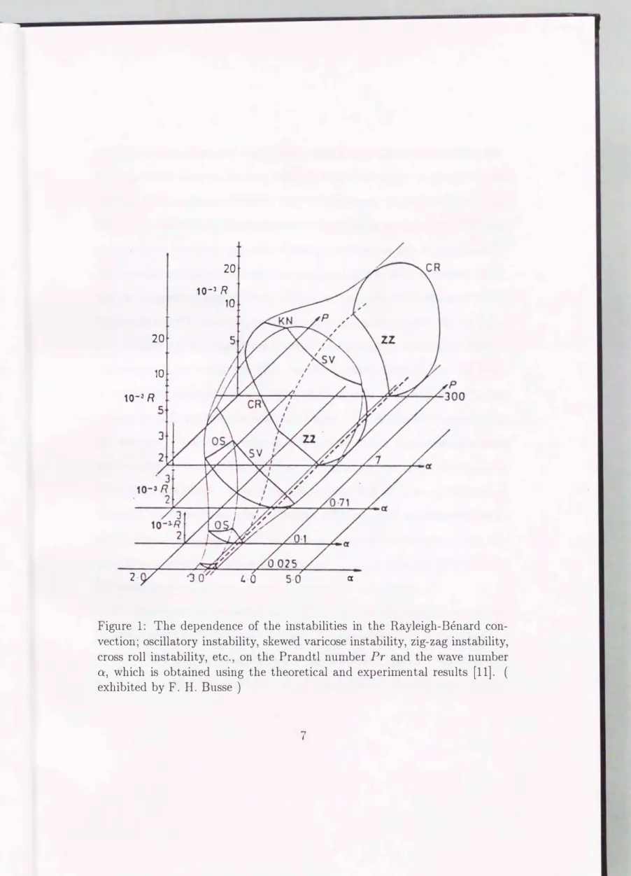
Busse et al. first studied how fundamental flow patterns can appear after the laminar flow becomes unstable[11],
and some instabilities: oscillatory instability, skewed varicose instability, zig-zag instability, cross roll instability, etc., can be observed with the different Prandtl numbers and the wave numbers. The dependence of their instabilities on the Prandtl numberPr
and the wave number a are exhibited in Fig.1,
which is referred to as the Busse balloon[11].
The oscillatory instability mainly appears in low Prandtl numbers, whereas, the zig-zag instability and the cross roll instability are important in high Prandtl numbers.This property indicates that the Rayleigh-Benard convection is a good model system for a comprehensive investigation of transport and diffusion,
20
10
10-3 R 5 J
2·
20
10-3 R 10
ex
Figure 1: The dependence of the instabilities in the Rayleigh-Benard con
vection; oscillatory instability, skewed varicose instability, zig-zag instability, cross roll instability, etc., on the Prandtl number Pr and the wave number
a, which is obtained using the theoretical and experimental results
[11]. (
exhibited by F. H. Busse
)
since convective flows can be created ranging from time-independent, spa
tially periodic flows on the one hand, to turbulent flows on the other. As a result, the transport rates vary over a wide range. At one extreme, when the fluid is motionless, the transport is due entirely to molecular diffusion.
At the other extreme
(
turbulent flows)
, transport is due to advection by the flow and is often described phenomenologically as eddy diffusion. There are two important laminar flow regimes between these extremes in a low Prandtl number: a time-independent and a oscillating regime. In the timeindependent regime, large-scale transport is limited by molecular diffusion between adjacent convection rolls. In the oscillating regime, the transport is dominated by advection of tracer particles across roll boundaries. In this regime, particle trajectories may be chaotic. The differential equation for the velocity of a fluid element in a two-dimensional, time-dependent flow are formally those of a Hamiltonian dynamical system with 1.5 degrees of freedom. As a result, the particle trajectories exhibit a lot of features of Hamiltonian chaos in real space. Chaotic structures such as heteroclinic tan
gles, invariant tori and islands have been observed numerically. Here, the quantitative effects of chaotic advection on transport and diffusion shall be discussed extensively.
In the present paper we shall especially show how the diffusion and mixing of passive particles by chaotic advection become anomalous when islands of tori exist
[21, 22].
We shall use the stream function used by Solomon and Gollub to simulate the particle motion. They defined the diffusion constantD in terms of Fick's law for the purpose of comparison with the experiment, measuring the value of D at most only for one complete period of oscillation.
On the contrary, we shall adopt the statistical-mechanical definition of D which is determined by the asymptotic behavior of tracer particles over a long time. It is shown that the difference noted above causes important changes of the dependence of D on the amplitude B. In particular, there appear some fine-grained peaks in D vs B graph
[21]
which were not found by Solomon and Gollub. This peak structure is understood as the result of an enhanced transport of tracer particles which can be explained in terms of certain structures of the invariant manifolds in fluid space[21].
It is further shown as an extreme case of the enhanced transport that, in a peak range of B, there appear accelerator-mode islands on which particles move fromx == =r=oo to x == ±oo in the horizontal coordinate with a definite speed, so that the intermittent sticking to the islands leads to an anomalous diffusion with D == oo
[22].
When they appear, the statistics of particle motions is dramatically changed and so physical quantities, too, as clarified recently for the standard map[25].
The formation mechanism of the accelerator-mode islands will be elucidated in terms of the lobe dynamics developed by Wiggins et al[26, 27].
As noted above, tracer particles diffuse in a widespread chaotic sea and this can be regarded as a stochastic process in a coarse-grained scale in spite that the dynamics is deterministic. This comes from an important feature of particle orbits in fluid space, i.e., the orbital instability due to the
exponential expansion of nearby particle orbits which leads to the mixing of tracer particles
[20].
The existence of the mixing is indispensable for the presence of diffusion. The degree of mixing is quantified by the positive Liapunov exponent. The distribution functionP(A;
n)
of the coarse-grained expansion ratesAn
gives us much more information on the particle orbits. In this thesis we shall also discuss the asymptotic form ofP( A;
n)
in the limitn ----* oo, and elucidate the anomalous mixing due to the coexisting normal
islands. It should be noted here that, though each of the chaotic particle
orbits is unstable against a small perturbation, their statistical properties over a sufficiently long time are stable and reproducible so that the statistical properties of particle orbits over a long time can be studied by computer simulation
[2
3]
.The present paper is organized as follows. In § 2 a review of dynamical systems is described. Here, the definitions of the Poincare surface, unstable and stable manifolds, pips and lobs, etc., are given. The lobe dynamics noted here will play an important role of understanding the diffusion process from a deterministic point of view. In § 3 an experiment and a simulation by Solomon and Gollub are reviewed. In § 4 we describe the dependence of the diffusion constant D on the amplitude B of the roll oscillation of the velocity field, and discuss the fine-grained peaks. These results are compared with Solomon and Gollub's results, and the differences are elucidated. In § 5 we show the existence of accelerator-mode islands in a peak range of B and describe a few characteristics about them. In § 6 we treat the enhanced
diffusion and the accelerator-mode islands in terms of the lobe dynamics reviewed in § 2. In § 7 we discuss the spectrum 1/J(A) and the probability density P( A; n
)
of the coarse-grained expansion rates An when islands exist.These quantities will show an anomalous scaling in this regime. A summary is given in § 8.
2 Review of Dynamical Systems
In this section, definitions and some properties for the equations of the fol
lowing form are summarized:
dx
/ dt
=f ( x, t; J.L) (2.1)
or
x r-+ g
(
x;J.L) (2.2)
where xis aD-dimensional vector,
t
means 'time' andJ.L
are some parameters which control the properties of(2.1)
or(2.2).
We refer to(2.1)
as a vector field or ordinary differential equation, and to(2.2)
as a map or a difference equation. When(2.1)
is solved with an initial condition x0, a family of the orbitsx(xo,t;J.L)
or{xo,x1,x2,···}
is obtained, and the family is referred to as a dynamical system.2.1 Poincare map
The study of the continuous time systems
(2.1)
is reducible to the study of an associated discrete time system(2.2),
by taking the Poincare surface[1].
Nowadays virtually any discrete time system that is associated with an ordinary differential equation is referred to as a Poincare map. This technique offers several advantages in the study of ordinary differential equations, including the following:
• Dimensional Reduction. Construction of the Poincare map involves the elimination of at least one of the variables of the problem resulting in
the study of a lower dimensional problem.
• Global Dynamics. In lower dimensional problems ( say, dimension:::;
4)
numerically computed Poincare maps provide an insightful and striking display of the grobal dynamics of a system
[29, 30].
• Conceptual clarity. Many concepts that are some what cumbersome to state for ordinary differential equations may often be simply stated for the associated Poincare map.
An example would be the notion of orbital stability of a periodic orbit of an ordinary differential equation
[12].
In terms of the Poincare map, this problem would reduce to the problem of the stability of a fixed point of the map, which is simply characterized in terms of the eigenvalues of the map linearized about the fixed point as noted below.The ordinary differential equation is easily reduced to a Poincare map in the case where the phase space of the equation is periodic , such as in period
ically forced oscillators. We consider the D-dimensional ordinary differential equation
(2.1)
and let¢(t,x;p)
denote the solutions of(2.1),
which form a one-parameter family of cr' r �1'
diffeomorphism of the phase space.¢(t,x)
is referred to as a phase flow or just a flow[13].
Let� be anD-1-
dimensional surface transverse to the vector field at
x0
(note: "transverse"means that
f(x)
·n(x) -=/= 0
where " ·" denotes the vector dot product andn( x)
is the normal to � atx )
; we refer to � as a cross-section to the vector field(2.1 ).
We can find an open set V C � such that the trajectories startingin V return to :E in a time
T (13].
The map that associate points in V with their points of first return to :E is called the Poincare map, which is in terms of¢( t,
·;J.L)
denoted as follows,(2.3)
where
T(x)
is the time of first return of the point x to�.¢(T(x),x;J.L)
is related withf( t, x; J.L)
as{ T(x)
¢(T(x),x;J.L)
==x
+l o f(t,x(t);J.L)dt. (2.4)
Here after the properties of
(2.2)
is only stated because of the remark men- tioned above.2.2 Fixed points and their stability
Consider a general D-dimensional difference equation
x
1---+g(x), x
E RD.(2.5)
When a point
x0
is chosen, the orbit ofx0
under the map(2.5)
is given by the infinite sequence{-
· ·, f-n(xo),
· · ·, f-1(xo), Xo,
· · ·, fn(xo),
· · ·} ,
andfn(xo)
is referred to as
Xn·
An fixed point of(2.5)
is a point x E RD such thatx ==
g(
x), (2.6)
1.e., a solution which does not change in time. Then, roughly speaking, the fixed point x is stable if orbits
{Xi}
starting "close" to x at a given time remain close to x for later times. It is asymptotically stable if nearbysolutions actually converge to x as t � oo. A fixed point is unstable if it is not stable. If x is an unstable fixed point, then there exists at least an orbit
{ Xn}
starting close to x at a given time and escaping from x for later times.In order to determine the stability of x, we must understand the nature of solutions near x. Let x = x +
y,
and substituting it into(2.5)
and Taylor expanding about x gives(2.7)
in terms of x = g
(
x)
, where Dg is the derivative of g and1·1
denotes a norm onRD. (2.7)
from which higher order terms are removed describes the evolution of orbits near x. Dg(
x)
is, in this case, a matrix with constant entries, and the solution of(2.7)
through the pointy0
of n = 0 can immediately be written asY
n-
_eDy(x)ny 0· (2.8)
Namely, if the eigenvalues of the associated linear map have not moduli one, then the orbit structure near on the fixed point of the nonlinear map is essentially determined by the eigenvalues
[13].
Let x be a fixed point of
(2.5).
Then x is called a hyperbolic fixed point if none of the eigenvalues of Dg(
x)
have Moduli one. A hyperbolic fixed point of the map is called a saddle if some, but not all, of the eigenvalues of the associated linearization have moduli greater than one and the rest of the eigenvalues have moduli less than one. If all of the eigenvalues have moduli less than one, then the hyperbolic fixed point is called a sink, and if all of theeigenvalues have moduli greater than one, then the hyperbolic fixed point is called a source. If the eigenvalues have 1nodulus one, the nonhyperbolic point is called a center. It should be clear that the fixed point y ==
0
of the linear map(2.7)
is asymptotically stable if all the eigenvalues ofDg(x)
have moduli strictly less than one, which means thatx
is a sink. On the other hand, ifx
is source or saddle, then the fixed point is unstable.2.3 Invariant manifolds
We will see that invariant manifolds, in particular stable and unstable man
ifolds, play an important role in the analysis of the structures of dynamical systems. We will restrict a discussion of these ideas only to a map
(2.5).
LetS C
RD
be a set. S is said to be invariant under the mapx
Hg( x)
if for anyxo
E S we havegn(x0)
E S for alln.
We remark that ifg
is noninvertible, then onlyn � 0
makes sense, although in some instances it may be useful to consider g-1. An invariant setS CRn
is said to be an invariant manifold if S has the structure of a differentiable manifold. Roughly speaking, a manifoldis a set which locally has the structure of Euclidean space
[14].
The stable and unstable manifold of a fixed point
x, ws(x), wu(x)
are defined by[30]
W8(x)
=={x
ERDign(x)--? x
asn--? +oo},
Wu(x)
=={x
ERDig-n(x)--? x
asn--? -oo }, (2.9)
respectively. It is easily shown in terms of the above definition that the set
ws(x)
is invariant under the map X Hg(x).
For any X EW8(x), gn
0g(x)
==gn+1(x)
�x
as n � +oo, and sog(x)
is also an element ofW5(x),
or equallyg(W5(x))
is a subset ofws(x).
We can also show thatws(x)
is a subset ofg(W8(x))
with the similar way. The two relations:g(Ws(x))
cws(x)
andws(x)
::Jg(Ws(x)),
say thatws(x)
=g(W5(x)).
By repeating the above process, the relation is easily generalized toW5(x)
==gn(W5(x))
for any n, and henceW5(x)
is an invariant set.Two stable
(
or unstable)
manifolds,ws(xl)
andW5(x2)
of distinct fixed pointsx1, x2
cannot intersect each other. IfW8( xi)
andW5( x2)
intersect at a pointx,
thengn(x)
�x1
in the limit n � oo since xis an element ofW5(xl),
at the same time,gn(x)
�X2
in the limit n � oo since X is also an element ofW8(x2).
As a result, existence and uniqueness of solutions of(2
·5)
ensure thatws( xi)
nws( x2)
==0.
On the other hand, intersections of stable and unstable manifolds of distinct fixed points can occur, and indeed, are a source of the complex structure of phase space found in dynamical systems. If there exists an intersection x of stable and unstable manifoldws(xl), wu(x2),
then there also exist infinite intersections{gn(x)}
for all n, sinceW5(xl)
andwu(x2)
are invariant under the mapg.
We then illustrate a separatrix as a simple example of
ws(x)
andwu(x).
We limit, for simplicity, a system with one-degree of freedom i.e., a vector field on a two-dimensional phase space, that have a first integral that can be viewed as the sum of a kinetic and potential energy. As a preliminary step, the shape of the potential
V( x)
is assumed to be a double-well potential where a coordinate(x, y)
==(0, 0)
is the maximum. Now suppose that thefirst integral is given by
and then
y
=±v'2Jh- V(x). (2.10)
Our goal is to draw an orbit with
h
=0.
Imagine sitting at the point(0, 0),
with
h
fixed. Now move toward the right, i.e., letx
increase. Then, sincey
=+ /2 J h - V ( x)
andh
is fixed,y
must increase until the minimum of the potential is reached, and then it decreases until the boundary of the potential is reached. In the case thath
is equal to the maximum value, all the points{x(t),y(t)}
reach a fixed point{0,0}
in the limitt
---t -oo; hence the set{x, -!2J-V(x)}
is an unstable manifoldwu (o, 0).
Nowy
=+J2Jh- V(x)
to
-V2J h - V ( x)
as time increases, and in the case ofh
=0,
the points{x(t), y(t)}
also reach the fixed point{0, 0}
in the limitt
---t oo; hence the set{x,/2J-V(x)}
is also a stable manifoldws(O,O).
Sincewu(O,O)
isaccordance with
W8(0, 0)
in this case,wu(o, 0)(
=ws(o, 0))
forms a loop including the fixed point{0, 0}.
All the points on the loop reach{0, 0}
inboth the limit
t
---t ±oo, and the orbit is sometimes called a separatrix, since it is a boundary between two distinctly different types of motions. Namely, ifh
is grater than the maximum value0
of the potential energyV ( x),
thenthe particle go around the right- and the left-well. For
h
<0,
within the potential well, the value of initial energy corresponds to bounded motion.The separatrices and the generalized ones will play an important role of analyzing the transport and the diffusion of tracer particles.
2.4 Pips and lobes
Consider a two-dimensional map g with a control parameter f..L
(2.11)
with a hyperbolic periodic point
Po,
i.e., for some integer k �1, gk(Po) =Po·
Without loss of generality we can assume that k
= 1
by applying our argument to gk rather than g. As an additional technical assumption we suppose that g is orientation preserving, i.e., detDg > 0. If g does not preserve orien
tation, then we apply our argument to g2, which does preserve orientation. It is natural since Poincare maps arising from vector fields preserve orientation.
We assume that an separatrix exists on some value of f..L. When 1-L is changed, the separatrix often separates into an unstable and a stable manifold of the fixed point
Po, Wu(Po)
andW8(Po)
, respectively, and the manifolds often intersect transversely. We denote one of the intersection points as q, and the point is said to be homoclinic toPo
or simply a homoclinic point. IfW8(p0)
and
Wu(Po)
are transversal at q, then q is called a transversal homoclinic point. Consider an orbit of q under g(2.12)
Since q lies in both
W8(p0)
andwu(p0),
and these manifolds are invariant, the infinite number of points in(2.12)
must lie in bothW8(p0)
andwu(p0).
Therefore,
W8(p0)
andwu(p0)
must wind amongst each other intersecting along the infinite number of points given in(2.12).
This geometrical structurehas been called a homoclinic tangle, and we now develop the concepts to describe it more quantitatively.
Let
U[g-1(q), q]
denotes the segment ofwu(p0)
with end points atg-1(q)
and
q.
ThenW8(p0)
intersectsU[g-1(q),q]
atq
andg-1(q)
and also at k points in betweenq
andg-1( q)
with k � 1 for orientation preserving maps.Without loss of generality we can assume k = 1, and easily generalize our results for k > 1. We denote the segment of
W8(p0)
with endpoints atq
and
g-1(q)
byS[g-1(q), q].
Here we call a special ty pe of homoclinic pointq
as a primary intersection point or pip defined as follows. Supposeq
Ews(p0)
nwu(Po).
Thenq
is called a primary intersection point(pip)[15]
if, other thanPo, S[po, q]
andU[po, q]
intersect only in the pointq.
The following lemma[26],
which is easily proved, is quite useful.Lemma. If
q
is a pip, thengk( q)
is a pip for any k.Lemma determines how to iterate of
U[g-1(q), q]
andS[g-1(q), q]
withg,
and of a lobeL,
which is defined as follows. Letq
andq1
be two adjacent pips i.e., there are no other pips on
U[q, q1] (
or equivalentlyS[q, q1]
)
betweenq
andq1.
Then we refer to the region bounded byU[q, q1]
andS[q, q1]
as a lobe. For any lobeL, f..L(L)
will denote the area ofL.
From lemma and the invariance ofW8(Po)
andWu(Po),
it follows that, for any lobeL, gk(L)
is also a lobe for any k. However, besides the pips, there are other secondary intersection points or sips which complicate matters further.Consider the lobes labeled
£1
and£2
in Fig. 2. Then, for positive integers k and n sufficiently large,gk(LI)
must cut throughg-n(L2)
as shown in Fig. 2.Po
, ,,',,.-····
;
g-l(q)
.././
' ... _ ....... - ,- ,' ,'
.--·/ Ll _../
, .
, .
R1g(L2,1 (1) )
........
..L2
. . . ·- - - . . . .-:>
_ _ _ _ _ _ _ _ _ _ _ ...
g(L1,2(l)) q
Figure
2:Stable and unstable manifold, W5(p0), wu(p0) are shown with
lobes £1, £2, g(£1,2(1)), g(L2,1(l)).
Let
X
=gk(LI)
ng-n(£2);
thengn(X)
=gn+k(£1)
n£2
is contained in£2.
Therefore, iterates of lobes will intersect other lobes. Here we note the main difference between pips and sips. Namely, once a pip enter a neighborhood of the hyperbolic fixed point under iteration by
g,
it remains in the neighborhood. Sips, on the other hand, may enter and leave the vicinity of the hyperbolic fixed point many times before finally remaining near the hyperbolic fixed point under all forward(
or backward)
iterations byg.
We then formulate the transport of particles in terms of the dynamics of the lobes. The term "separatrix" in the map having transversal homoclinic orbits is generalized as follows. Choose any pip
q
EW8(po)
nwu(Po).
Then the region bounded byU[p0, q]
US[p0, q]
is referred to as a pseudoseparatrix[26].
Note that ifW5(p0)
nwu(p0)
contains one pip, then it contains an infinity of pips. Therefore, there are infinitely many choices for the pseudoseparatrix. The obvious question thus arises as to which choice should be made. This depends on the context of the specific problem under consid
eration. In dealing our problem, it is probably most natural to choose the pseudoseparatrix so that it is as close as possible to the separatrix in the associated integrable problem.
We assume that the phase space is divided into two disjoint components, labeled
R1
andR2,
by choosing a pseudoseparatrix. The problem of transport in phase space that we shall study is concerned with how initial points inR1
may enter
R2.
It will be shown that this is completely determined by the geometry and dynamics of the lobes. We suppose thatS[g-1(q) , q]
intersectsU[g-1(q),q]
in precisely one pip besidesg-1(q)
andq,
as shown in Fig. 2.Then precisely two lobes are formed, one lying in
R1
and the other lying inR2,
which we denote byL1,2(1)
andL2,1(1),
respectively. Nowg(L1,2(l))
andg(L2,1(1))
appear as in Fig. 2. Note thatL1,2(1)
entersR2
under one iteration byg,
andL2,1(1)
entersR1
under one iteration byg.
This is the mechanism for transport across the pseudoseparatrix and appears to have been discussed explicitly for the first time by Channon, Lebowitz[16]
and Bartlett[17].
The lobes bounded byU[g-1(q), q]
US[g-1(q), q]
have been called a turnstile by Mackay, Meiss and Percival[35].
The mechanism for transport noted above reveals that initial points in � enteringRj
on the n-th iterate ofg
must bein
Li,j(l)
on the(
n -1)
iteration ofg,
withi,j
= 1,2.Now we can obtain an important quantity concerning the transport in phase space across the pseudoseparatrix . The area of phase space crossing the pseudoseparatrix from
R1
intoR2
under one iteration ofg
is given byp,(g( L1,2)).
Thus, the total area of phase space crossing the pseudoseparatrix fromR1
intoR2
under n iterations ofg
isnp,(g( L1,2)).
The quantity we want to obtain is the area occupied by points that are inR1
initially(
i.e., at t = 0)
that enterR2
on the n-th iteration byg.
The quantity is notp,(g(L1,2)),
because we are not just interested in arbitrary points crossing the pseudoseparatrix but, rather, in points which have a specified location initially. Thus, with each point in the plane it is important to keep track of whether it was inR1
orR2
initially. The points lying in Ri at t=
0 will becalled � particles. Heuristically, we can think of
R1
particles as black fluidand
R2
particles as white fluid, and we are interested in how the fluid mix amongst each other under the dynamics generated byg.
We first establish some definitions. LetLi,j( n)
denote the lobe that leaves � and entersRj
on the n-th iterate and let(2.13)
thus we have
(2.14)
The main quantity that we wish to compute is a flux of
Ri
particles intoRj
on the n-th iterate, which is given from these definitions by
(2.15)
Next we want to compute
Li,2(k).
Using an observation noted above,R1
particles can not enter
R2
on the k-th iterate unless it is in£1,2(1)
on the(k -1)
iterate. Thus, points in
g-k+1(L1,2(1))
enterR2
on the k-th iterate. However,g-k+1(L1,2(1))
may not contain onlyR1
particles, sinceg-k+1(L1,2(1))
may intersectg-1+1(£2,1(1)),
l = 1,···,k, and, thus, lie inR2.
Hence we haveLi_2(k)
=g-k+1(L1,2(1))- k-1 U (g-k+1(L1,2(1))
ng-'(£2,1(1))).
1=0
Now, since the sets
g-k+1(L1,2(1))
ng-1(£2,1(1))
are disjoint, we havef1(gn(Li,2(k)))
=f1(gn-k+1(L1,2(1)))- k-1 L J1(gn-k+1(L1,2(1))
ngn-l(£2,1(1))).
l=O
Thus the flux
J1(gn(Li,2(n)))
is obtained as[26]
J1(gn(Li,2(n)))
=f-l(g(£1,2))- n-1 L f-l(g(£1,2(1))
ngn-k(£2,1(1)))). (2.16)
k=O
We make an important remark that
(2.16)
has implications for all points in R1 but are obtained entirely by iterating the turnstile. The formula will be used in§ 6
and play an important role of elucidating the diffusion process of the Rayleigh-Benard convection from a deterministic point of view.2.5 Dissipative and conservative systems
The D-dimensional differentional equations dx
/
dt =f (
x)
are called dissipative systems when the phase space volume is continuously contracted with increasing time, and then the contraction rate is given by \7 ·
f
< 0. This leads to contraction onto a surface of lower dimensionality than the original phase space, and the surface is referred to as the at tractor. For regular motion, the at tractor of the flow represents a simple motion such as a fixed point
(
sink)
or a singly periodic orbit(
limit cycle)
. For flows in two-dimensions there are , in fact, the only possibilities.For three-dimensional regular flows, in addition to sinks and limit cycles, quesiperiodic orbits may be possible. In addition to these simple attrac
tors, it has been shown that attractors exist for dissipative flows in three
or more-dimensions that have very complicated geometric structures. These structures can be characterized as having a fractional dimension, and are usu
ally called strange attractors. The rnotion on strange attractors is chaotic or critical.
On the other hand, the differentional equations are called conservative systems or Hamiltonian systems when the phase space volume is conserved,
which satisfy the condition
V' ·f(x) =
0,or detDg = 1 in the case of a map
g. If a 2n-dimensional equation is determined by a Hamiltonian function
H(q,p, t) as
BH/Bpi, i=1,···,n, (2.17) then the equations always satisfy the conservative condition as follows,
v.
f(x) = t�(-BH)
+�(BH)
= o.i=l Bpi Bqi Bqi Bpi
Consider a time-independent Hamiltonian system H0(q,p) with n-degrees of freedom. If there exist n-independent invariants of the motion, then the system is called integrable. It is well known as the Arnold theorem that the flow of the integrable system with n-degrees of freedom forms n-dimensional tori. We then consider a 2n-dimensional integrable system that is perturbed slightly . If the perturbation is sufficiently small, the KAM theorem [18]
guarantees the existence of invariant tori. The theorem says that if the linear independence condition of the frequencies is satisfied with over some domain of phase space, then the perturbed motion is much less than the
unperturbed one and the invariant curves, which is called KAM-invariant
curves, exist near the unperturbed orbits. In the region that the condition
is not satisfied, chains of alternating elliptic and hyperbolic fixed points are
found with regular phase space trajectories encircling the elliptic fixed points
and invariant manifolds connecting to the hyperbolic points. The stochastic
behavior of the map around the hyperbolic points is found and is understood
due to the sequential stretching- and folding processes in phase space, and the processes are visualized with the homoclinic (or heteroclinic ) tangles of the invariant manifolds.
The transport property of particles are, as noted above, analyzed in terms of the lobe dynamics. The Hamiltonian system has neither sinks nor sources, and hence the lobe dynamics will be more simple
[26].
We again limit to the map g with detDg == 1. In this case we have(2.18)
and
(2.19)
Substituting
(2.18)
and(2.19)
into(2.17),
and reindexing givesf.l(L
i
' 2(n))n-1
J-l(LI,2(1))-
2:
J-l(LI,2(1) n gk(L2,1(1))),(2.20)
k=l
where we have used the fact that by construction L1,2(1) n L2,1(1) ==
0.
Inwords, the sets L1,2(1) n gk(L2,1(1)) are the points that leaves R1 and enter R2 under one iteration by g subject to the condition that they entered R1 from R2 k iterations earlier.
3 An Experiment on Diffusion by Solomon and Gollub
Solomon and Gollub have studied the transport of tracer particles in nearly
two-dimensional, time-periodic Rayleigh-Benard convection experimentally and numerically
[
20]
. In their paper qualitative observations of the transport rates are presented, along with quantitative measurements of the transport rates as a function of the strength of the time dependence. A simplifiednumerical model is discussed in which transport between convection rolls is caused by chaotic advection due to lateral oscillations of the roll boundaries.
Then the model gives a semiquantitative account of the experimental results.
3.1 Diffusion of tracer particles in Rayleigh-Benard convection
The convection cell used in their experiments is a rectangular box with hor
izontal dimensions 15cm
(
along the x direction)
by 1.5cm(
the y direction)
and a depth of 0.75cm(
z direction)
. The working fluid is water at an average temperature of 36 oc, where the Prandtl number is 4. 7. Convection patterns are established with rolls oriented parallel to the short side of the convection cell. To obtain spatial information about the flow it is necessaryto collect velocity time series at locations along the convection cell. The time average value of the vertical velocity Vz at each location is then used to describe the spatial structure of the flow, and the standard deviation < e5 v >
averaged over a wave-length of the flow is used as a measure of the local
amplitude of time dependence. After injection of an impurity, which is r - ferred to as tracer particles elsewhere, one-dimensional concentration profiles
c
( x, t)
averaged over y and z direction are measured at the midhight of the cell. An enhanced local-transport coefficient is defined using Fick's law for a coarse-grained concentration profilec(x, t):
ac(x, t)
F(x, t)
==D(x, t) ax , (3.1)
where
F(
X't)
is the flux of dye past the point X att
andacj ax
is determined by measuring the slope ofc( x, t)
between the centers of adjacent convection rolls. The enhanced diffusion coefficientD(x, t)
is determined by dividingF(x, t)
byacjax.
Transport experiments were performed at Rayleigh number
R
ranging fromR/ Rc
== 19(
just above the onset of time dependence in this cell)
through
R/ Rc
==32.
HereRc
is the Rayleigh number corresponding to the onset of convection. Visual observation of the motion of an impurity injected through a small tube in the bottom corner of the cell clearly indicates the presence of advective transport between convection rolls. Small blobs of the impurity are pulled periodically from the corner of one roll into the next.Lines of impurity are stretched and folded repeatedly in the vicinity of the corners. Stretching and folding of this nature are common characteristics of chaotic maps in which a rectangle in phase space is stretched and folded onto itself. Within the rolls, impurity concentrations are found to homogenize very rapidly. This time is short compared to the typical time of approximately one-half day for the experiments.
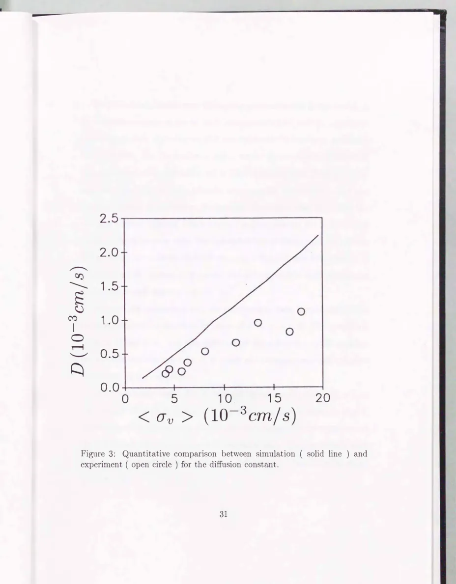
Transport coefficients are measured for each run in terms of (3.1), which is found to be independent of time, within the resolution of the data. There is a monotonic relationship between
Dand
< O"v >which we determined experimentally. Plots of
Dvs
< O"v >are shown in Fig. 3 with open circles.
An approximately linear relationship can be seen from these plots .
3.2 Elucidation in terms of Lagrangian turbulence
A simplified model of transport in time-periodic Rayleigh-Benard convection is, then, described. A Lagrangian approach is taken in which the trajecto
ries of individual tracer particles are obtained by integrating the equations describing the velocity field. The system is Hamiltonian: dx ( x, z, t) / dt and dz(x, z, t)jdt are derived from a stream function
\ll(x, z, t)
=(A/k) sin{k[x
+Bsin(wt)]}W(z), (3.2)
where A is the maximum vertical velocity in the flow, k is the wave number 2n-j)..., and W ( z) is an even function of z that satisfies the rigid boundary con
dition at the top and bottom surfaces. W(z) is obtained by solving the hydro
dynamic equations (1.2) strictly [28]. This stream function describes single
mode two-dimensional convection with rigid boundary conditions. B
=0
corresponds to the flow where the Rayleigh number
Ris below the onset of
the time-dependent instability. To study the flow above the onset, the term
B sin( wt) is inserted, and the term represents the lateral oscillation of the
roll pattern with amplitude B and frequency w that is caused by the even
oscillatory instability [19].
2.0
�
r:IJ
� 1 .5
� u
M
1.0 I
0
r-f0.5
...__..,.
Q
0.0
0 5 10. 15 20
< CJv > (10-3cm/ s)
Figure
3:Quantitative comparison between simulation ( solid line ) and
experiment ( open circle ) for the diffusion constant.
Trajectories of particles near the separatrices are chaotic in this model. A quantitative comparison can be made between the model and the experimen
tal transport data. Calculations of D as a function of
B
have been performed for the model. The parameters A and w are set to match the conditions of the experiment. One convection roll is filled uniformly with10000
particles, and the trajectories of these particles are computed individually. After one complete period of oscillation, the number of particles that have been exchanged between adjacent rolls is counted to determine the net flux
F(x,
t)of tracer particles between rolls. The calculated flux of tracer particles and the difference in concentration between the rolls is inserted into Fick's law(3.1)
to determine D. Values of D are determined numerically for amplitude of oscillation
B
such that0
<2B I
A <0 .1.
For a proper comparison with the experimental data, the strength of the oscillation should be expressed in terms of< CJv >, not
B.
The convection betweenB
and < CJv > is accomplished by expanding thefJz I
&t equation for smallB,
determining CJ v( x, z)
atz
==0
and averaging over one complete wavelength of the roll pattern.It is numerically found that D depends linearly on
B (
and < CJv >)
for small values of2B I).. ( 0 ::; 0.1 ) .
A plot of D vs < CJv > is shown in Fig.3.
The results of the numerical model are presented along with the experimental data. For both the experimental and numerical data, D scales linearly with
< CJv >. The slopes of the experimental and numerical data differ by about a factor of
2.
D
to-1
• • • • • •_.'
r
•
•
•
•
•
B
l
•
. ,
•
. .
• •• •
. I
• •
· .
1
10-1
•
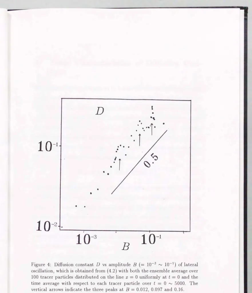
Figure
4:
Diffusion constant D vs amplitude B(
=10-3
f'.J10-1)
of lateral oscillation, which is obtained from( 4.2)
with both the ensemble average over100
tracer particles distributed on the line x =0
uniformly at t =0
and thetime average with respect to each tracer particle over t =
0
f'.J5000.
Thevertical arrows indicate the three peaks at B =
0.012, 0.097
and0.16.
4 Some Characteristics of Diffusion Con- stant
The diffusion constant D measured by Solomon and Gollub is reflected only in properties of a few periods of motion, as reviewed in §
3.
We now examine the long- time behaviors of tracer particles governed by the same stream functionas Solomon and Gollub, which is nondimensionarized, to be invariant under the transformations
{ x, z}
-+{ x ± 2, z}
and{ x, z}
-+{ x ± 1, -z}.
Using the well-known Poincare-section method we take the plots of the orbit{x(t), z(t)}
of each particle at discrete time
t = 0, ±1, ±2,
· · ·,
which are denoted by Xt ={
Xt,z
t}
with a two-dimensional Poincare mapXt+l
= g(Xt). (t = 0, ±1, ±2,
· · ·) ( 4.1)
This system is equivalent to a Hamiltonian dynamical system with
1.5
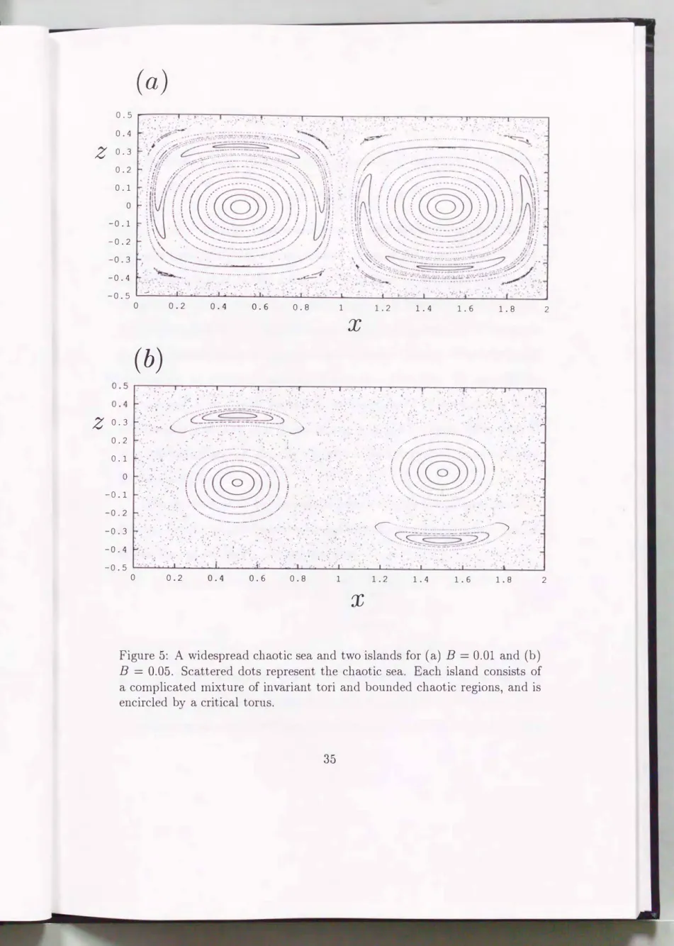
degreesof freedom, exhibiting invariant tori, islands of tori, and chaotic seas
[29, 30].
There is a widespread chaotic sea generated by the oscillating roll boundaries, in which tracer particles move from roll cell to roll cell successively
[20, 21, 22].
In the following we shall consider chaotic orbits of such particles in thewidespread chaotic sea, and study what effects the islands of tori bring about on their diffusion and mixing.
The motion of each particle in this chaotic sea is characterized as a dif
fusion process in the horizontal direction because the memory of its initial point is lost rapidly due to the mixing of particle orbits, and can be regarded
0.5 0.4
z
0.30.2 0.1 0
(a)
. . ,. .: . ..
_·, .. :
;
. ·• '.· . . ,. ...
: . -�. -.: ::. :. . ._.,,'.:.· "'
· · ..... :·:::.:..:-�...
. .
-·- -·- -·- --
_,·'
,..--..----: ---...
-0.1 -0.2 -0.3 -0.4
·· ..
\\��;d�, '
.·
�
·. �
.j :
,
� ; ��"� � : ; : � � � � a : ..•..
-0.5 ':
.
:.:.:. ·;·:.z
0.30.2 0
(b)
0.2 0.4 0.6 0.8 1
X
1.2 1.4 1.6
__ ,,·
· ....
1.8
a . ' .. o •, o •
.... -. ··
·., . ; . . . . � _ · _ _
:
·,/ /;.;
..
----·· ·----<<
. ,··\ ..._:::
. .. .. '
· ..-.: . ( \,· '( -,s���-:< { �) :)) ./,.
··.. .
.·::: '::
. . ·. · . ..\
.... (\ i> �.J) ;
. -.
. .. ·:
···· ..
-0.2
-0.3
. . '' .· r._.·,:
-0.4 -0.5
. · · : .
·.:�. r···... . . ... ···)
...
:
· .. . c�<:�::�-=:2�---) .
. · .-·.·..
.2
0 0.2 0.4 0.6 0.8 1 1.2 1.4 1.6 1.8 2
X
Figure 5: A widespread chaotic sea and two islands for
(
a)
B = 0.01 and(
b)
B = 0.05. Scattered dots represent the chaotic sea. Each island consists of a complicated mixture of invariant tori and bounded chaotic regions, and is encircled by a critical torus.