ハミルトン系におけるトーラスの島による異常な拡 散と混合

九州大学学術情報リポジトリ

Kyushu University Institutional Repository

ハミルトン系におけるトーラスの島による異常な拡 散と混合

石崎, 龍二

九州大学理学研究科物理学専攻

https://doi.org/10.11501/3065447

出版情報：Kyushu University, 1992, 博士（理学）, 課程博士 バージョン：

権利関係：

Thesis

Anomalous Diffusion and Mixing

due to Islands of Tori in Hamiltonian Dynamical Systems

Ryuji ISHIZAKI

Department of Physics, Kyushu University 33, Fukuoka 812

December, 1992

Abstract

Anomalous behaviors of the diffusion and mixing of chaotic orbits due to the intermit- tent sticking to the islands of normal tori and accelerator-mode tori in a widespread chaotic sea are studied numerically and theoretically for Hamiltonian systems with two degrees of freedom. The probability distribution functions for the coarse-grained velocity ( ^charac-

terizing the diffusion) and the coarse-grained expansion rate (characterizing the mixing)

turn out to obey an anomalous scaling law which is quite different from the Gaussian. The scaling law is confirmed for both diffusion and mixing by numerical experiments on the standard map and the heating map. Its scaling exponents for the diffusion and mixing, however, are found to be different from each other, indicating that different islands give different scaling exponents.

Contents

§1. Introduction - reconsider classical mechanics by chaos

§2. From regular motion to irregular motion of frictionless penduhun

§2.1 The simple pendulum

§2.2 Simple harmonic oscillator and forced oscillator

§2.3 The periodically kicked rotator

§3. Anomalous diffusion in the standard map

§3.1 Deterministic diffusion

§3.2 Anomalous diffusion due to accelerator-mode islands

§4. The behavior of a small cell in phase space in the heating map

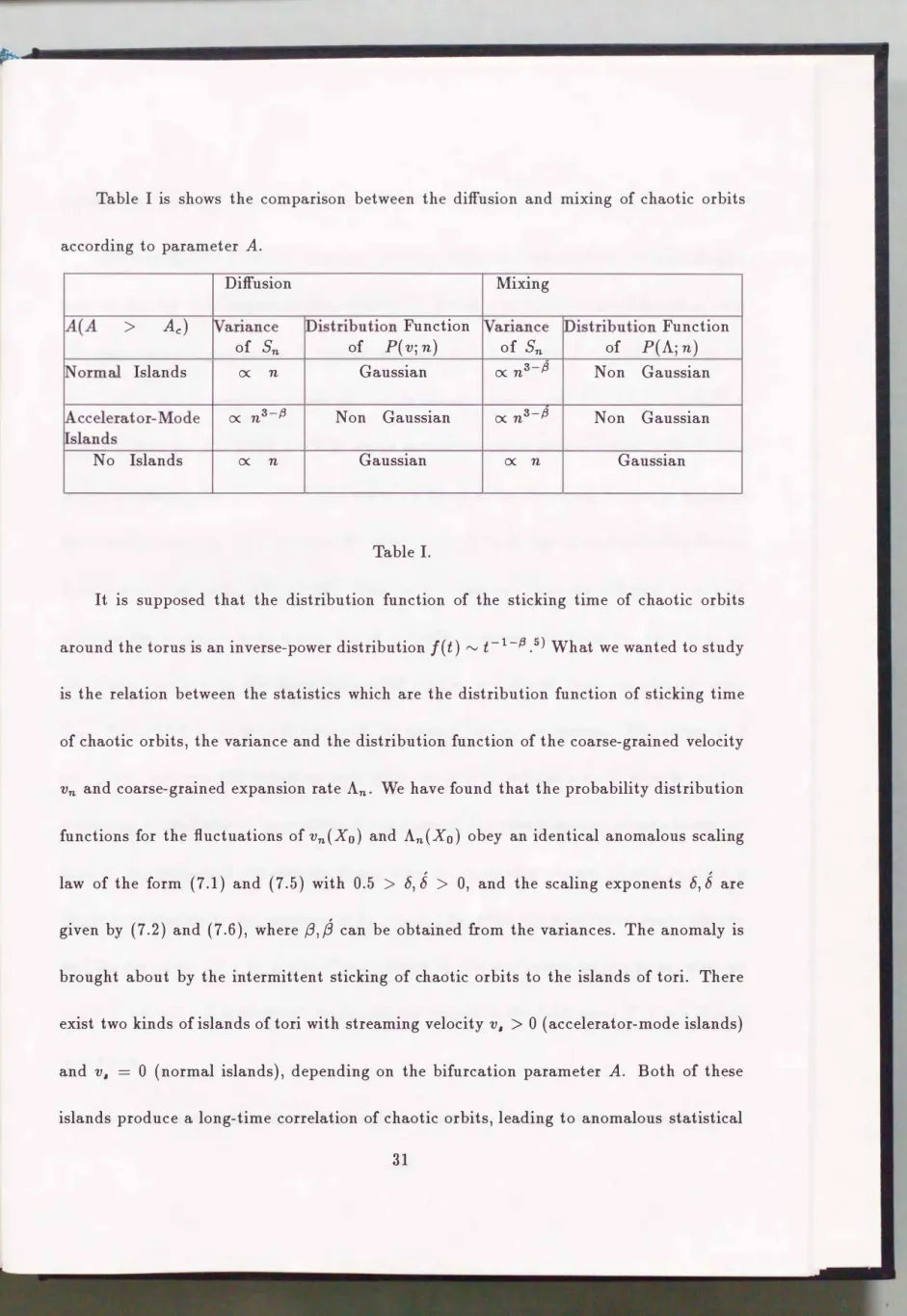
§5. Diffusion and mixing of chaotic orbits

§5.1 Diffusion and velocity spectrum ,P( v)

§5.2 Mixing and expansion-rate spectrum ,P(A)

§6. Numerical results

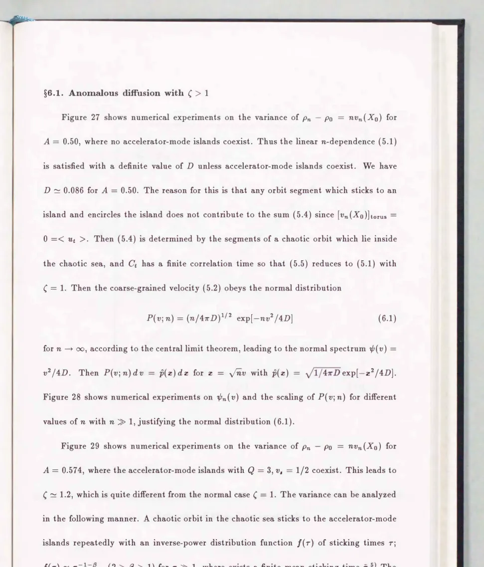
§6.1. Anomalous diffusion with ( > ¹

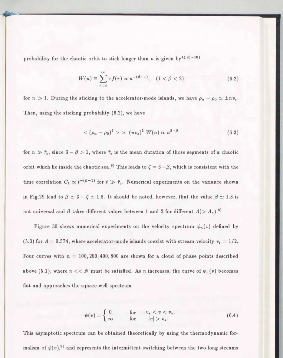
§6.2. Anomalous mixing with

(

§7. Anomalous scaling law for P(v;n) ^and P(A;n)

§7.1. P(v; n) ^for -v, ^< v ^< v,

§7.2. P(A; n) ^for A> ⁰

§8. Sununary and remarks

Acknowledgements Appendices A,B,C References

§1. Introduction - reconsider classical mechanics by chaos

One of the purposes of this thesis is to understand the motion of a frictionless pen­

dulum. It may be said that "That needs no explanation at this time". To be sure, the frictionless pendulum continues to oscillate in constant rhythm as regular as clockwork.

As soon as a periodic external force acts on the pendulum, however, the motion becomes complex. In a particular case, the motion becomes very complex, and the future of the motion is not able to predict. It is common sense that we can not predict the future, when the many factors are generally involved in it. But in this case, we can not predict the future though rule is clear, and the degrees-of freedom are only two and the external force is not random but regular. This strange phenomenon is called chaos.1)"'3)

The discovery of chaos has greatly influenced science. Let us first review the repre- sentative studies and the meaning of chaos in science.

Look back on the history of science, it was Newton to indicate that we can predict the behavior of matters if we know the rule of the motion. Kepler's laws explained how planets move around the sun. In contrast to this, Newton tried to explain the motive power which causes such a motion. He guessed from the law of inertia and Kepler's law that the planets continue to be pulled by the sun. He found that the intensity of the force is in inverse proportion to the second power of the distance between the sun and the planet. Kepler's law has been completely explained by his theory. He also guessed that the attractive force acts between the earth and the moon, and explained the phenomena of tide. He guessed

--�-

further that all matters on the earth are pulled by the earth, and explained the free fall and the motion of pendulum, etc. Newton showed that the motive power of celestial motion and motions of matters around us are the same, and explained the time evolution of motion of matters. Then we have been able to understand the motion of planets, comets, moon and pendulum, etc. This is the so-called law of universal gravitation, where gravitation acts between all matters. He expressed the motion in the differential equation and showed that we can understand the motion if we can solve the equation. By Newtonian mechanics, we can predict how the state of motion changes with time if we know what forces acts on the matter and know the motion state

(

)

We became to be able to understand behavior of matter by deterministic law. Physi- cists have simplified complex phenomena to understand them and discovered regularities in them. Irregularities have recently been discovered though they simplified things. Though rule is clear, it is not able to predict the future. That is due to chaos. As a remarkable example, let us take the Lorenz model.

Lorenz constructed a simple model to explain the complex motion of the atmosphere.

First, suppose a layer of fluid of infinite horizontal extent, heated from below, as shown in Fig.l

(

)

(

d3g1dT jva)

dT

d

g

1

v

2

(a) _T

d

T+6.T

(b)

J \

Fig.l

(

)

(

)

(a)

(b)

Fig.2 (a) Hexagonal convection cells on a uniformly heated copper plate in a circular con­

tainer and open to air surface. Fluid is silicon oil. Visualization with aluminum powder.

(E.L.

177 (1974)) (b)

tric rolls on a uniformly heated copper plate in a circular container and not open to air surface.

(E.L.

177 (1974))

becomes unstable and the regular convection appears, as shown in Fig.l(b). This is the so-called Rayleigh-Benard convection. The pattern of the convection is various whether the surface of the fluid is open or not to ambient air, as shown in Fig.2. As the temperature difference becomes larger, the transition to turbulence is observed. Lorenz assumed that the convection rolls are all parallel, as shown in Fig.l(b). Then he reduced the number of

variables that describe this system to three. The equations are X= -u + uY,

Y=-XZ+,.X-Y, Z = XY- bZ,

(1.1)

where X is the amplitude of the convection motion, Y the amplitude of the temperature fluctuation, Z a uniform correction to the vertical temperature profile, u the Prandtl number, ,. the normalized Rayleigh number and b a parameter related to the horizontal wave vector. These equations are the so-called Lorenz model. He discovered that these equations produce very complex motion. As a matter of surprising fact, the deviation becomes larger with time if the initial value is shifted a little, as shown in Fig.3. This means that the prediction of future is impossible because error of observation is rapidly magnified. This is called "sensitivity to initial conditions." Is this motion completely random, then? The dynamical motion is understood as the trajectories in the phase space.

Figure 4 draws the motion in the phase space. The motion whose time series look random produces a very symmetrical form in the phase space. This means that the Lorenz model produces complex motion in the very symmetrical form. He showed further the possibility

X(t)

10

0

-10

0

I' tl I' tl I' ,I II ,I I ' rl I ' I I I' I

I I I

L f II I I II ,,

�

tl II II I' ,, 11 I I II I I I I )

10

,,

\) II 11 tl II II II '

•

t 20

F

g.3

(

10,

X(t)

{X1

Y1

1

0.11,

27.0} (

line).

28,

8/3).

27.0} (

)

z

·' . ; .. : ·-· . ^/ . .. ·.·.·.·.:, ·,,

·'· ' • ·. · .. . .

X

Fig.4 Phase space {X, Y, Z} of the Lorenz model (0' 10, r 28, b= 8/3). The ong1n 1s {X 0.0, y 0.0, z 27.0}.

Zn+l

. ·�

t .

I

40

/ ..

l ^..

� '

I _'

I t _�

�· I

.. 1 . . . .

. . . .

30

,.

I I

30 40 Zn ₅₀

Fig.5 Zn+ 1 vs Zn, where Zi are successive maxima of Z for the Lorenz model

(

that the complex motion produced by many degrees-of-freedom can be understood as a chaotic motion with a few degrees of freedom. He observed that the change of the maximum in the Z-axis is represented by one dimensional map, as shown in Fig.5.

The famous example for one dimensional map is the logistic map,

X(n

1)

f(X(n))

aX(n)(1- X(n)). (1.2)

This is the model to understand the change of the individual number of each generation of a living thing. Parameter ^a expresses propergating power which is the ratio of children to parents. If the number of parents is too much, they finish feed on food and the number of children's generation decreases. The

(1 - X(n))

a.

a

ac(

)

The Lorenz model is the dissipative system which does not conserve energy and for which volume elements in the phase space shrink as time increases. What is chaos in the Hamiltonian system which conserves energy, then? As a remarkable example, let us take the Henan and Heiles system.

Henan and Heiles constructed a model to understand the motion of star which moves in the Galaxy. They supposed that the influence from the others of stars to a star in the Galaxy is represented by a potential and derived the following Hamiltonian

H ⁼

�(P;

P;)

� ^(X2

^Y2)

^(X2Y- � ^Y3),

4

(1

)

1 X(n)

�-�---1

0 n ₁₀₀

1

X(n)

0 1 ₀ n ₁₀₀

1 -

X(n) �� ������

0 0

0 . Xn 1 ₀ n ¹⁰⁰

1 1

--�

(a4) (b4)

� � �� t� N ^{M � �}

Xn+l X(n)

-

Fig.6 The behavior of the logistic map for

(al)(bl)a

(a2)(b2)a

where the third term represents the influence from the others of stars. They observed the crossings in the Py

-

(

0,

0)

What mechanism breaks the smooth curves? Kolmogorov, Arnold and Moser consid- ered about the condition that the regular orbits survive when the nonlinear perturbation increases and obtained the following KAM theorem. The regular orbits are stable, if the ratio of the system's frequency w1 to the external force frequency w2 satisfies the following condition

{1.4)

under the perturbation cH1 in the limit f. < <

1,

/

The practical example of the KAM theorem which is seen in the nature is the motion of asteroid between Mars and Jupiter. The asteroid continues to be perturbed by Jupiter and are swept in the orbits in which the ratio of the unperturbed frequency of the asteroid motion w to the angular frequency of Jupiter Wj becomes rational, as shown in Fig.8.

This is the Kirkwood Gap. The existence of stable asteroid orbits can be considered as a confirmation of the KAM theorem. It is also guessed that the gap in the ring of Saturn will be originated by the same mechanism. In particular, the Cassini division which is the

5

0.2

-0.2

(a)

, .. .. # -·

)

,.7

�, . . ^{. ··} ... , .·· . . ·· ·�. � '

,.' !

....

:

:

.:::

I f :· \_.·:· .. ·· ^·'' .- ', �\

: : . : .·' , ' ' ·'

=: ^..

. ,. 'o'�·

• ^. f ^. • ^{I '}

� \ I ^{' a}

\ _{� \ '·} ^\ _{"- / I I} ^{l •}

• ^{' ...__, I #}

� !'·',

�.

.

,· l ^{·. · . . ... ,' .... ..}... ...,....r.#,

\ � ·. . . . .. ' ' ,,

' \ ·. • . j' . ·--·-··· ^••

\ �' J

)

... � -··

-0.3

0.4

-0.4

-0.5

(c)

. .. . · ..

,... . ·r . .,

, ···\ . ..

,: • • ^.&. • • • • ••

. ....:· .· . ··.� ..

I •

.•• ... ) ^; • : • ^{• •' \}

c. .......

.

.

. . · .

,..,.

.

" .:, ^#

( -�-=

)\

'-� ·, .. · _.... ·� ---...--...^{.. ./} . }

� .. ^_... ___,

. .

. -.

. ..

.

• • { • ... ) • • ^: • • :, I

' ' . ,

.. · _.... .

. .

. ··. ;^·; . . . ,·:

• • ^{\ I}

. ·: ·-:·. �· .

y

0.4

0.8

0.4

� _. , .. ., _. .

(b)

..

.. . .)

I# ^• • • ^•••

.

. .

..

' .

-0.4 -0.4

0.6

-0.6 -0.6

• . I \. .. / ··:. ·• • • .. ·-·· ·. · ..

.

.· ^-.,; - .. " '·.

: .

.

�

• •. ^{. ' '·}

.

.

. . ...

,

.

....

{... . .. ·-· ·· .

·. ·... . .

.

.

• ' ••• ^.,..J ••••• ••

' .

. ..

y

(d)

. .. . .. . ·.·

. ... . .

... · .· ^I, • ' . ^{. . . :- � · .} . .. ^. , . ^. .. . . .• . . .

.:

• • ^• • w.:,. r . 'f 'rJ..))'.

\ ) ' ... .:! •• ,^.. ... � ':'..^{. : • • •}

. .

: .<·:

? :;:,

• •

.

.

. ·. · .

. . .· : .... ··

..

• ., ^{.I •}

. . ^. . ,

.

y

0.6

1.1

Fig.7 Poincare maps of the Henon-Heiles system for

(a)E

1/24, (b)E

1/12, (c)E

1/8

and

(d)E

1/6.

5 50

('j u

E 0

,.-

l

3:1

2.0

i l r

5:2 7:3 2: 1 3:2

i i

i

Jupiter

3.5 astronomical unit 5.0

Fig.8 Distribution of asteroids in the belt between Mars and Jupiter. The gap is due to

perturbation of Jupiter.

(P.Moore, G.Hunt, !.Nicolson, P.Cattermole, The Atlas of the Sola,. System

(Mitchell Beazley Publisher (₁₉₈₁))

-

(a)

(b)

1 00

1 2J Dring Fig.9 (a) The ring of saturn.

C ring

(b) The group of ring.

Bring

Cassini division A ring

The gap is due to perturbation of satellite.

F ring

= 110.000 2 8 G ring

E ring

(P.Moore, G.Hunt, !.Nic olson, P.Cattermole,

The Atlas of the Solar System

(Mitchell Beazley Publisher ( 1981))

gap between A ring and B ring is due to the perturbation of the satellites which go around the ring of Saturn.

The theory of relativity and quantum mechanics were constructed to explain the phenomenon which can not understand by Newtonian mechanics. The relativistic theory is produced from the question what is the medium which transmits light. The relativistic theory made clear that the phenomenon looked by observer is different by observer's motion state. The quantum mechanics was constructed from the question how to explain the facts that the behavior of matter in the micro scale looks like either particle or wave according to the way of observing. The quantum mechanics made clear that the place and momentum of particle in the micro scale can not be observed at the same time and we can know only the existence probability of particle.

Due to these theories, Newtonian mechanics is the classical mechanics and physicists considered that there is nothing to study in the Newtonian mechanics. By the discovery of chaos, however, classical mechanics became to be reconsidered. Because it is recognized that the simple systems which seemed very simple produce very complex motion. Then the studies of complex motion produced by simple rule became active.

In this thesis, we shall consider on the behavior of frictionless pendulum. In particular, we shall study the anomalous behaviors of the diffusion and mixing of chaotic orbits caused by islands of normal tori and accelerator-mode tori by taking the standard map and the heating map since they exhibit remarkable statistical properties clearly. In §2, we would

6

introduce how the behavior of frictionless pendulum is changed by external force. In §3, we consider the deterministic diffusion in the standard map which gives a model for the complex behavior of frictionless pendulum. In §4, we look at the behavior of a small cell in phase space in the heating map. In §5, we introduce the coarse-grained velocity ^v and its spectrum

1/J(

)

A

,P(A)

A

§2. :From regular motion to irregular motion of frictionless pendulum

§2.1 The simple pendulum

Let us consider the motion of the simple pendulum, where one edge of the weightless stick of length

l

m

m

mg

and tension S from the stick act on this mass. The equation of motion is

mld2() I dt2

-mg

(2.1)

where() is the angle between the stick and the vertical line. The integration of this equation by time is

(d

1 dt)2

(2g ll)

(2.2)

o

m

mg y

Fig.lO The simple pendulum.

Fig.ll Phase space {B, B}

the simple pendulum.

C = W� - (2gjl)(1-^COS 0), _{Wo =} 0 _(at 0 ₌ 0).

If Wo is larger than 2

ViJI,

§2.2. Simple harmonic oscillator and forced oscillator

Let us consider the motion of mass m putted on the spring, as shown in Fig.12. The spring stretches to the point 0 due to the gravitation mg. When the restoring force is proportional to the deviation from the point 0, the equation of the mass m is

(2.3)

where ^z is the upward deviation from the point 0 _and k is the spnng constant. This equation is equivalent to the simple pendulum's equation which the maximum value of 0

is very small (sin 0 ::: 0). The general solution of this equation is

X(t) =A cos(wot + _o:)_{, (2.4)}

where A is the amplitude, w0( =

�)

Vmfh

m X

0

Fig.l2 The mass ^m putted on the spring.

x(t)

x(t)

Fig.13 Phase space { z, z} of the simple harmonic oscillator.

t

In the next, let us consider that the external force

F(

)

F0

( wt)

(2.5)

The general solution

(

F(t)

0)

(

)

A

(w0

+a).

X

(

)

(

)

- m(w�-w2) '

Then the general solution of this equation is

X

(

)

A

(wot +a)+ Fo

( 2 2)

(

)

m w0 -w

(2.6)

(2.7)

If the angular frequency

w

wo,

w

wo.

w

w

w0,

w

wo.

But this does not happen because there is the limit of shirink of spring or the force does not proportion to the deviation in this case. It is called the resonance at the case

w

wo.

§2.3. The periodically kicked rotator

Let us consider the periodically kicked rotator where the periodic external force acts on the frictionless pendulum with no gravitation, ^as shown in Fig.14. The equation of

F(t)

Fig.14 Kicked Rotator.

motion is

00

d2()jdt2=-Ksin() L

8(t-nT), (2.8)

n=-oo

where K is the strength of the external force. The rewritten equations with J ( ⁼

B)

{ ^dJjdt

t;

^8(t-nT),

d()jdt

(2.9)

If the external force does not act on the rotator( K ⁼

0),

(2.9)

{

^{- �}

(2.10)

for the variables

(2.11)

by integration. This map is the so-called standard map1) introduced by Chirikov. Figure

15

{

16

0.8.

15,

J

-0.5

0.5

J

-0.5

-0.5 ()

• •• • •• • •0 • • • • • • • • 0 .

. . . .

•• 0 . . .. . .. 0 • • • • 0 • • • • • • •

. . . .

• •• • ••• 0 • • •• • • • • • • • • • • • • • • • • •• • • • • • •• • •

. . . . . . . . . . . . . . . . . . .

. .

.. . . .. . .. . .. . . . . . . . . . .

• • • • • • • • • • • 0 . 0 • • 0 •• •

• • • • • • 0 •• • • • • • • •

. .

. . . .. .. . .. . .. . . ..

. . .

. . . . . . . . . . . . . . . . . . .

. . .

-0.5

(b)

0.5

()

0.5

-0.5

0.5

-0.5

(a)

() ^0.5

(c)

Fig.l5 Phase space {0, J}

the standard map

(a)

(b) K

and (c) K

0.4

J(n)

0

-0.4

0 n ¹⁰⁰⁰

Fig.l6 The evolution of

of the standard map forK

The initial point is {

0.001

}.

0.5

(a)

J

e 0.5

(b) (c)

0.057

•'. ,

..

·:,= ·

J

� ^':

:':' -,: :.::;J!f/i{l ijf: i :·i:

0. 05 2 !�,�,s�:����������1- �1 :} .:·-

0.372 () 0.437 0.409 f) 0.414

Fig.l7 Phase space {B, J} for (a)

(b) The magnification of the box of (a). (

) The

magnification of the box of (b).

any chaotic sea is in contact with the critical tori encircling islands of tori whose Liapunov exponents are zero. In particular, when the region of the boundary between torus and chaotic sea is magnified, it can be seen the chains of small islands around each of the critical tori which have the islands-around-islands hierarchy, s) as shown in Fig.17. Any chaotic orbits are often trapped by such a hierarchical structure in the chaos border and stay there for a long time, since the local expansion rate of nearby orbits is nearly zero around the critical tori. Such sticking of chaotic orbits to the islands occurs repeatedly and intermittently, and causes a long-time correlation of chaotic orbits.5) Hence the chaotic motion is not perfectly random.

The chaotic motion in Hamiltonian systems is thus neither perfectly random nor regular. How this motion can be characterized? It should be noted that, though each of chaotic orbits is unstable against a small perturbation and hence unreproducible, the ensemble average of chaotic orbits over a cell as well as the long-time average over each chaotic orbit are stable and reproducible so that the statistical-mechanical properties of chaos can be studied by computer simulation.4)

§3. Anomalous diffusion in the standard map

§3.1 Deterministic diffusion

For K > Kc = 0.971635406 ^{· · ·}, all the KAM tori which connect () ⁼ -0.5 to () = 0.5

disappear,4) as shown in Fig.18(b). In this parameter range (K > Kc), there exists a

(b)

J

-1.5

-0.5 () 0.5 0.5

Fig.18 Phase space {0, J} for (a) K = 0.8 where exist the KAM tori which connect 0 ⁼ -0.5 to 0 ⁼ 0.5, and (b) ^K

=

..

1

J(n)

0

- 1

0 n ³⁰⁰⁰

Fig.l 9 The evolution of J of the standard map for K ⁼

1.2.

{

0.0,

0.001}.

1.5

1.0

0.5

0 20 K 50

Fig.20 The normalized diffusion constant D

/ ( t ^K2)

K

The dots are the nun1erically computed values and the solid line is the theoretical result.

(

(1980), 1586)

widespread chaotic region which includes the unstable fixed points

( er =

J; =

This means that the action

Jn

Jn

Jn

P( J; n)

Jn(Xo)

J.

{Jn}

P( J; n)

{)P(J; n) {)2 P(J; n)

8n =

{)J2 '

where D is the diffusion constant. Then if Dis obtained, then we can know the statistical properties of action

Jn(Xo).

§3.2 Anomalous diffusion due to ac celerator-mode islands

This is considered due to particular periodic points which are so-called accelerator modes. We consider the periodic points before we explain the accelerator modes.

The linearized matrix of the standard map are

M ₌

[�

Eigenvalues of matrix M are

- K

21r(}n l

1

K

21r(}n .

A± ₌

2- K

21r8n

)(2- K

27r8n)2- 4

2 .

The stability condition for

{Jn, Bn}

12

K

21r(}n I

2.

The period

1

{ ^J;

(}�

0, 0.5.

The linearized matrix M about fixed points are

M ₌

[�

_=r:K ^{K .} l

The stability condition for fixed points yield

12

Kl

2.

(3.2)

(3.3)

(3.4)

(3.5)

(3.6)

(3.7)

Thus the point at

81

0.5

K

4

81

0

1

K

4.

For a general map,

(}

1

J

J

1.

13

period 1 fixed point. If we consider that the phase and action (both mod 1) are stationary, then we put

K . ()* l

- Sln 2 7l' 1l = ,

271' ^m, l : integers. (3.8)

Thus period point is named accelerator modes because the action at the fixed point in- creases by l for every iteration. The stability condition is replaced by

and then

(3.9)

Islands exist around the periodic point and islands exist around islands in the Hamiltonian systems. The chaotic orbits are trapped by islands when the chaotic orbits approach the islands. When the chaotic orbit enters between islands, it is difficult to go out from this region because of the infinite hierarchical structure of islands. Then the motion is regular for a long time. The action J of chaotic orbit increases by constant interval for this interval. Then the diffusion is enhanced. The structure of islands around the accelerator mode changes as the parameter K is varied, as shown in Fig.21. The accelerator-mode islands are created around a stable periodic orbit {X;}, (t ⁼ 1, 2, ^{· · ·,} Q) with period Q,

which satisfies16)

(3.10)

0.1

(a)

J

-0.1

L_--�---�---

0.19

e

(b) (c)

0.1 0.1

J J

·-0.1 -0.1

0.2

()

()

Fig.21 The structures of the islands around the accelerator modes for (a) K ⁼ 6.4717, (b)

K ⁼ 6.5973, (c) K ⁼ 6.9115.

where

l

{ x;}

(3.9)

Q

1.

mode islands for a long time, then the action J of the chaotic orbit increases by step

Va ⁼

±v,, (v,

lli/Q)

§4. The behavior of a small cell in the phase space in the heating map

In relation to plasma heating by the radio-frequency wave, it is known that chaotic ion motion arises due to the nonlinear interaction of the resonances between the cyclotron motion and the wave. Karney demonstrated that the equations of motion for ions in a lower hybrid wave can be well approximated by a two-dimensional conservative map and showed that the motion produced by this map becomes chaotic.

The interaction between the cyclotron motion and the wave can be schematized as shown in Fig.22. The equations of motion for an ion in the plane

{z, y}

( 4.1)

where n is the cyclotron frequency. If the ion motion does not satisfy the wave-particle

E

Eoxcos(kxx- wt)

y

r

X

®

B

Boz

Fig.22 The motion of an ion with mass ^m and charge

q

0(

qBo /

)

(

j

^{il /0.).}

X

---- - ---- -

-r

X w/kx

X

® Bo

Fig.23 An ion orbit in phase space

{

{Bt,pt}

{Bt+l,Pt+l}

resonance condition

z

w / k�,

(z2

iJ2)112 jO.

wfk�O

{z{t),z{t)}

{4.1) to the two-dimensional conservative map for

Xt

{ut,vt}, (t

[ ^Ut+l _Vt+l ]

^F(Xt)

[ _Vt ^Ut

⁽

^vt) l

cos

{

ut+l) '

( 4.2)

where

Pt

Ot

Pt

Ot

{

()

()

p

p

{

and the time reversal

t

-t,

- ()' p

p.

Hence the phase-space structure in

{ (), p}

()

as shown in Fig.24. In the following we shall take d ⁼ 0.47. Then for A> Ac = 0.20565 ... ,

all the KAM tori which connect

()

()

Pt

Pt

Pt

16

1.5 (a)

p

1.5

- 0.25 e 0.75

Fig.24 Phase space

{B,p}

A> Ac = 0.20565 ... if dis fixed to bed= 0.47.

There is also accelerator-modes because p is periodic by 0.5. The accelerator-mode islands are created around a stable periodic orbit {X;}, (t ⁼ 1, 2, ^{· · ·,} Q) with period Q,

which satisfies17)

Q-1 Q^-1

L

L

i=O i=O

( 4.5)

where m and n are integers with m + n being a nonzero integer. The periodic points x;

move to p = ±oo by iteration with definite velocity ^{Va =} (p;+Q - p;) / Q ⁼ ±v,, ( v, ⁼ lm + ni/2Q) in action p. The range of A in which the accelerator-mode islands exist is determined by the stability condition of the periodic orbit { x;} and is given by Az < A <

A 1.1. with 17)

Az ⁼ Max(lm- dl, In+ dl),

( 4.6)

for Q ⁼ 1. If a chaotic orbit sticks to the accelerator-mode islands, staying among the hierarchical structure of chains of small islands around the accelerator-mode islands for a long time, then the action Pt of the chaotic orbit increases by step Va = ±v, every iteration.

In order to elucidate how the state point moves in the chaotic sea, let us take a widespread chaotic sea and consider the behavior of a small cell in it that represents numerous state points. Figure 25 shows the time evolution of a thin cell in phase space

17