近畿大学学術情報リポジトリ
19
0
0
全文
(2) 74. CHARACTERISTICS OF SIMIS Hardware requirements of SIMIS is a standard personal computer with a CPU of 80386 or faster with a minimum hard-disk capacity of 40 Mb. The program is written in dBASE IV (version 4.1) programming language and works under a dBASE IV environment. SIMIS is composed of 14 modules considered important in irrigation management and operation as shown below. "Project Support" and "Project Management" menus are the core of the program and each has many modules (independent program for managing and processing of information) _ The Project Support menu stores basic information necessary to manage and operate and irrigation system, and information processing is mainly carried out in the Project Management menu. Simplicity and adaptability are two features of SI:vns different from ordinary irrigation management software. The need for skilled professionals to operate and maintain computer software has made long-term use of software up to now. Obviously computer software should be simple and easy to use. In addition, the software should be flexible enough to cope with the conditions specific to each project environment so that it can be used in a variety of operating environments and countries.. Projeci Support. Projects. Exit. Report &. Printer sellings Passwords. Select Project Modify Project. ... \~·.:.r:r.~D1:..' aimale Crops Soils PbyslCllI lDfrultuCl\Jre Land Use &. Tenure Machinery. ..... Project Management Setup. '. Agricullural Adivities Crop Water RequlRments Seasonal Irrigation Plaooing Irrigation Seheduling Water Consumption Accounting , O&M AcliviUes - Costs Water Rates. APPLICATIONS OF THE IRRIGATION SCHEDULING MODULE In an assessment of the usefulness of the irrigation scheduling module and as part of a long·term simulation of different scheduling options, this module was applied to two irrigation projects, one in Argentina in an arid climate and with upland cultivation and the other in Thailand in a humid climate and with paddy monoculture. 1 Application to the Mendoza Project in Argentina 1.1. Outline of the Irrigation System One target irrigation system was in Mendoza Province, in the central west part of Argentina, There are five major irrigation districts in Mendoza with a total irrigated area of 360,000 ha. about 30% of the total irrigated area in the country. The Departamento General de Irrigacion (DGI) , an autonomous body for irrigation management, manages and distributes water together.
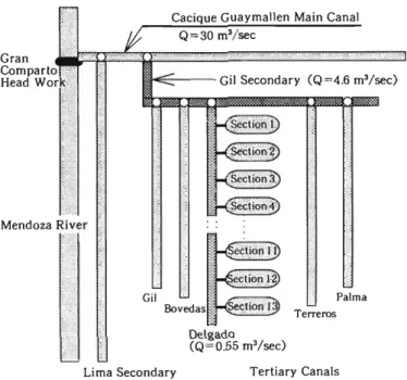
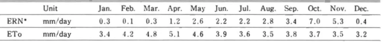
(3) HAT. 110:. 75. Irrigation Water :Vlanagement through Information Management Cacique Guaymallen Main Canal Q=30 m3/sec. Gran Comparlo '.'t:. Head Work~:::.. m--E--- Gil Secondary (Q=4.6 m3 /sec). Gi~' ~:t::. .{. ... :~;. :.~. ~. ,.;;. ) ;.~. ":::. :~:.. .$. Mendoza River. Palma. Gil. Terreros. Delgado (Q=0.55 m3 /sec) Tertiary Canals. Lima Secondary Fig. 1 1.. Layout of C. Cacique GuaymalJen Irrigation Sy tern. with the water users' associations (WUA). The DGI carries out operation and maintenance activities for major irrigation systems (reservoirs and primary canals) and the WUA is respon sible for secondary and more minor canals. The SIMIS irrigation scheduling module was applied to one tertiary unit, called the Hijuela (tertiary canal) Delgado, of the C. Cacique Guaymallen Irrigation System, which diverts water from the Mendoza River by the Gran Comparto Head Works. The canal layout of the system is shown in Fig.l-1. The total irrigable area of the sY:item is about 50,000 ha and the HijueJa Delgado has a total irrigable area of 386.5 ha, of which :~32.6 ha is cultivated. The irrigation water is allocated according to irrigation water rights (jrrigable area). In Menduza, irrigation is normally practiced continuously, but when the supply is low, rotational irrigation is practiced within sectors. 1.2. Climate, Soils, and Crops The climate of Mendoza is arid with a mean annual rainfall of 192 mm. Reference evapotran spiration (ETa) was calculated by the Penman-Montieth method and is shown in Table 1-1 together with the effective rainfall (ERain), calculated by fixed percentage (80%) of monthly rainfall because the area is arid and rainfall is light. There are two kinds of soil in this tertiary unit; one is sandy loam and the other is silt loam, with available soil moisture of 140 mm/m and 1,8 mm/m, respectively. Silt loam soil has a limiting soil layer that does not allow root penetration at 0.9 m, and sandy loam has such a layer Table 1-1. Climatic Data for Mendoza nit ERain'. mm/mom. ETo. mm/day. 'ERain:. jan.. F b.. l'vlar.. Apr.. May. jun.. jul.. Aug.. 32.8. 22.4. 21.6. 9.6. 4.0. 3.2. 3.2. 5.7. 4.8. 3.5. 2.4. 1.7. 1.2. 1.3. Sep.. Oct.. Nov.. Dec.. 2.4. 7.2. 16.0. 11.2. 19.2. 2.2. 3.1. 4.2. 5.2. 5.8.
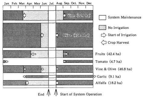
(4) 76 at 0.7 m. The soil data is used to calculate readily available moisture (RAM) at different crop-growth stages. Data on climate, soil, and agronomic characteristics of crops were obtained from the local research institution, the Instituto Nacional de Ciencia y Tecnica Hidricas (INCYTH). :'v1ajor crops grown in the area are vine, olive, fruits, alfalfa, tomato and garlic. Vine and olive are often inter-cropped. Vine, olive, and fruits are perennial crops different from other field crops because they are already planted at the start of the irrigation season. 1.3. Current Irrigation Management Practice In Mendoza, irrigation water is delivered by a supply-oriented approach. A supply-oriented approach to water management distributes water by division of the supply based on water rights or cultivated area_ Fixed dividers or division boxes are often used for dividing the flow into smaller units that correspond to the irrigated area or water right. The advantage of this approach is that management practice is simple and less demanding, and this approach is most used for irrigation water management worldwide. For simulation of water management practice by the supply-oriented approach, the available water is distributed according to the irrigable area of each minimum management unit (quaternary canal), defined as a section. All fields receive the same amount (depth) of water whether the field is planted and irrigated or not. The mean water application depth under certain supply conditions to the sector (tertiary unit), which is the group of sections in the same canal system, can be calculated as follows: Depth =0.0036 x Flow x Efficiency x Duration/Sector Area· (Equation 1) Depth: Mean water application depth (mm) Flow: Flow available to the sector (l/s) Efficiency: Distribution Efficiency from sector intake to field intake (%) Duration: Duration of irrigation assigned to the sector (h) Sector Area: Total irrigable area of the sector (ha) The mean application depth in Equation 1 is used calculate the needed duration of irrigation for each plot or field, and irrigation is done from one plot to the next for the assigned duration. In the supply-oriented approach, canal flow assigned to each section varies according to the irrigable area. The supply-oriented option in the simulation allows introduction of rotational irrigation within a sector. Fields and plots in the same sector can be grouped into several subunits, and total irrigation time to each subunit can be calculated from the area. Each subunit is irrigated with full flow to the sector but with shorter duration calculated from the irrigable area of each subunit. This option can be used when the available water is much less than the canal capacity, which causes large distribution loss. Irrigation starts in August with water released from a reservoir upstream of Mendoza River. When the flow allocated to the tertiary is small (from August to October and from March to June), the tertiary unit is subdivided into two and each subdivision is irrigated in rotation, each week to avoid inefficiently low flow in quaternary canals. At other times (from 1\ovember to February), the flow allocated to the tertiary is large enough for irrigation of the entire tertiary unit. Irrigation canals are closed in July for maintenance. There are 80 plots in the tertiary unit, with a total irrigated area of 332.6 ha. The cropping pattern of the area is shown in Fig. 1~2. The area of vine and olive accounts for more than three-Quarters of the irrigated area of the tertiary unit. Irrigation starts in August for olive, garlic, and alfalfa, and vine, fruits, and tomato receive water starting in September. Perennial crops such as vine and fruits have small irrigation needs after harvest and during the winter they are not irrigat d. Water diverted at the Gran Comparto Head Works passes into secondary and tertiary canals.
(5) HATCIIO:. 77. Irrigation Water Management through Information Management. D. System Maintenance. I>:::ll. No Irrigation. Q. Start of Irrigation. Q. Crop Harvest. Fruits (42.4 ha) t:Jl:lmi1~m1.l~. Tomato (4.7 ha). Vine & Olive (46.8 ha). ;;;;;~¢=;;;;;;;;*'Garlic. (9.1 ha). Alfalfa 08.2 ha) End Fig. 1-2.. ~ ~. Cr()ppin~. Start of System Operation. Pattern of Tertiary Canal Hijuela Delgado. and then through quarternary canals to fields with division according to irrigable area. 1.4. Simulation of Water Management by Different Scheduling Methods Current water management practice was simulated for 16 weeks by use of the supply-oriented option (Supply·Oriented Method: SOM) of the irrigation scheduling module starting in August. Fields are grouped into 13 sections by the location of intakes and sizes of the sections are described in Table 1-2. \Vhen the flow is small, the tertiary unit is subdivided into two subunits: the first subunit is of sections I to 6 and the :;econd is of sections 7 to 13. The first subunit is irrigated for 3 days plus 6.9 h and the second for 3 days plus 17.1 h according to their irrigable area. In addition, the management practices have been analyzed by demand-oriented approach. The major difference between demand-oriented approach and supply-oriented one is whether there is a variation of water supply to each section or not. Under demand-oriented approach, it is assumed that each section has an access to the water supply whenever demand arises. Since there are 13 sections in the tertiary unit, the maximum net water demand when all sections are irrigated is the product of 13 and the flow size assigned to each section (20 lis). Comparisons in terms of total irrigated volume, water losses, and possible crops damage are carried out among the 4 methods of scheduling: Supply-Oriented, Fix, Rational and Optimal. Current water management practice, as described above. was simulated by the Supply Oriented method. For the Fix method (Fix I), fix interval of 7 days and volume of 30 mm/application was applied to every plot regardle~ of the type of crop or growth stage. The Rational method (Rat 1) used the same 7-day interval, but the application depth varied according to the crop water Table 1-2. Groupings of PINS intCl Spctions. 2 Area" (hal "Area = Irrigable area. 4. 5. 6. 7. 8. 9. 5. 2. 3. 12. 19. 7. 5. 40.0. 22.2. 36.4. 27.6. :n_5. 25.9. 22.4. 3. 10. 11. 12. 13. 25.5. 23.4. 28.2. 44.6. 9.
(6) 7 requirements (CWR). The amount corresponding to the product of 7 and CWR at the planned irrigation date was used as an application depth. For the Optimal method (Opt 1), irrigation was planned when the soil moisture of a specific plot reached less than 20% of RAM and terminated at 80% of RA. 1. The range is arbitrary, but the lower range is set to keep a certain amount of water in the' soil bdore irrigation in order to avoid possible damage; the higher range, to maintain a certain storage capacity for possible rainfall. CWR is calculated by multiplying ETo with the crop coefficient in the Crop Water Require· ments module of SIMIS on a decadal basis. The result is used to calculate soil moisture balance (5MB) of each field so that effectiveness of water delivery can be analyzed. The equation used for calculation is listed below. M8t=SMBt-1 ERAINt IRRIGt~7XCWRt ················ .. ······························(Equation 2) 5MBt: Soil moisture balance at the week t (mm) 5MBt-1: Soil moisture balance of the previous week t-1 (mm) ERAINt : Effective rainfall of the we k t (mm) IRRIGt: :--let irrigation water application of the week t (mm) CWRt: Crop water requirements of the week t (mm/day) When 5MB goes beyond the value of RAM, a water loss is registered. When it drops below zero, the damage to crops is calculated by applying a yield response factor which is stored in the agronomic characteristic database.. 1.5. Results and Discussion 1.5.1 Comparison of water delivery by different scheduling methods The result of simulation are shown in Table 1-3. The first column lists the abbreviations of different scheduling methods. The number 1 after the abbreviation indicates different examples of the same scheduling method. Total supply (second column) is the water delivered to the intake of the tertiary canal. The relation among the columns is that Total supply is the sum of Delivery loss, Application loss (I). Application loss (II), and Net use by crop. Application loss (I) and Delivery loss is determined by the effici 'ncy values assigned by the user. In SINIIS, each section can have different application and distribution efficiencies, but the values of 80% for distribution efficiency and 70% for application efficiency are adoped in these simulations. Applacation loss (II) is the water lost due to over-irrigation beyond the limit of RAM as calculated by Equation. 2. Final soil moisture of the 8th column shows the mean soil moisture of all plots at the end of simulation. For Rat 1, total supply was small but the watGr remained in the soil was also small which could lead to crop damage at the time of long spell of drought. Table 1-3. Simulation of Water Delivery by Different Scheduling iVlethods Method. Total supply. Delivery loss. (unit). (m 3 ). (m 3 ). let crop use (m 3 ). Efficiency. Final soil moisture. Crop damage. (m 3 ). (%). (mm). (%). 33. 62.6. 0.4 0.04. OM. 2.375.65". 39.238. 461.399. 292.029. 782.990. Fix I. 2.357.500. 471.500. 565,272. 04.159. 816,570. Rat I. 1.160.695. 232, 1:39. 278.883. 70. 649.603. 35 -6. 67.1 16.9. 0.02. Opt I. 1.231.147. 246,229. 295.607. 1. 689,310. 56. 28.7. 0.03. SOM: Supply-Oriented Method of Scheduling. Fix: Fix IVlethod of Scheduling (7-day illl~rYal, 30 mm applica· tion) l~at: Rational Method of Scheduling (7 day interval and variable applications), Opt: Optimal Method of Scheduling (interval and application based on 5MB). Applic. Loss (I) : Water loss assigned by the user by Application Efficiency. Applic. Loss (II) : "rater loss by over irrigation.
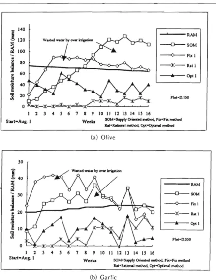
(7) Irrigation \Vater ;Vlanagement through Information Management. HATCIIO:. ......- - R A M --O--50M. -j. 80. ~. 60. ~Fixl. --::!:--Ral. '". Cpl.. 1~ :I. 20. ;t-::K-::K~""::K. ::K-::K-::Kc.:b.::K.d::,.r~. o J. 2. 3. 4. 5. 6. 7. Swt-AUI- I. PI"'-D.ISO. ,. 8 9 10 II 12 13 14 I~ 16 Woeb 30M-Supply OrioolIod...cbod, 1"". ..., .. medlod Rol-Rotionol mdhod. 0pI-()ptnW medlod. (a) Olive. 50. ----RAM --O--SOM. --<>--',,1 -::K--R.oll '". 0pI1. PI"'-D.050. I 2 Swt-Aug. I. 3. 4. 5. 6. 7. 8. 9. w..Ja. 10 II 12 13 14 13 16. SOM-:><.w1y Orionod .-hod, Yi><-Fix melhod IUl-RotionoI method, 0pl-Opt.... 1 medlod. (b) Garlic Fig. 1-3.. Soil Moisture Balance of Different Scheduling Methods. Al11on~ four scheduling methods, SaM and Fix I methods used a volume of about 2.4 million m 3 whilt' Rat 1 and Opt 1 methods used only half as much. Delivery loss with SaM came from water allocated to plots which were not planted or cropped becau'e water right is the principle of water allocation. Nearly 35% of water withdrawn is due to distribution loss; 20% is general distribution Joss, which is defined by the user. and the remaining] 5% is lost by irrigating above RAM level and assigning water to non· irrigated plots. Comparison was made between the volume of waleI' supplied and water stored in the root zone of a crop. The amount of water used by crop is the difference between the water entering into the root zone and that which was wasted because water supplied went over the limit of RAM. Overall irrigation efficiency, which was calculated by dividing the volume of net crop water use by total supply volume, was about 56% for Opt) and Rat] methods. :~5% for Fix] and 3:~o for SaM. S:YIB calculated by Equation 2 was used to as'e possible water loss s and crop damage. S\'i!3 on a weekly basis is shown in Fig. 1-3 for two plots under different scheduling methods. The crops are olives and garlic, which have different characteristics. The variations of S IB for 16·wc:~'k period is shown by the lines with different marks; those' of RAM by a thick line. For. 79.
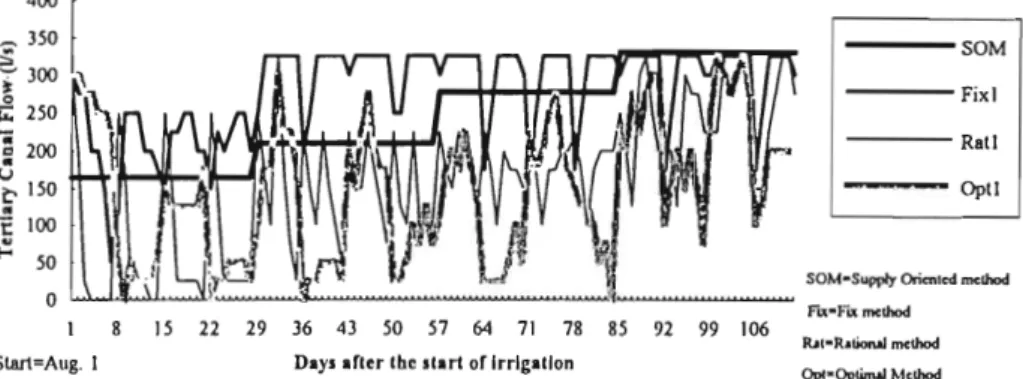
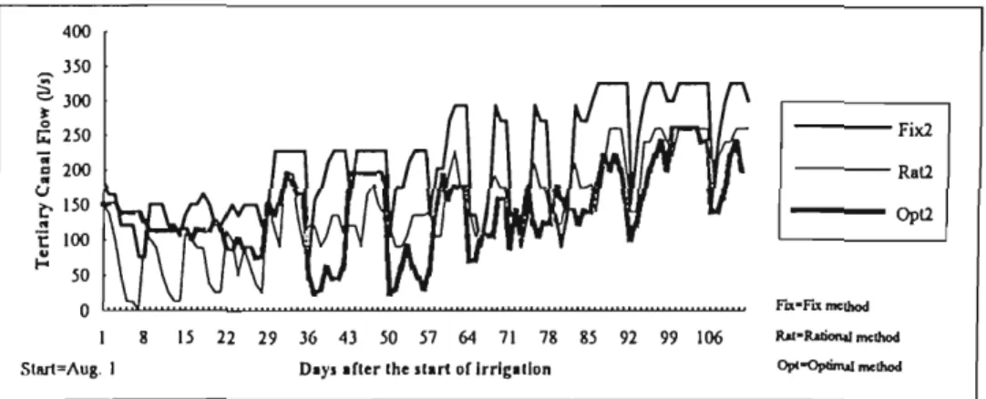
(8) 80 the 50:\.1 and Fix 1 methods, it is easy to see in Figure 1-3 how fields are over-irrigated beyond the level of RAM. When the crop had relatively small CWR at an early stage of growth and RAM was small with minimum root development, water could be easily wasted by the SOM or Fix 1 method because supply did not reflect CWR at a specific growth stage. The 'Lolume of overirrigation for the Fix 1 mothod can be decreased by reducing the amount of application depth from 30 mm to 20 mm, for example. However, in a peak demand period, this could lead to crop damage. Possible crop damages shown in Table 1 3 are at most 0.4% of total maximum yield, which is relatively small for all methods. This is because of the relatively short interval (7 days) adopted (except for Opt 1) method and the large application volume which resulted in water losses rather than crop damage. It is important to note that over-irrigation could result in a rise in the water table and waterlogging and salinization in arid and semi-arid areas, In Mendoza region, salinization is a serious problem, which can be tackled by more precise application of water based on a demand·oriented approach of irrigation scheduling, 1.5.2. Canal operation schedules Based on the irrigation scheduling and irrigation time ordering of each plot, canal operation schedules were calculated. Under SONt, flows assigned to each section are variable, determined by the available supply and water rights allocated to each section. The other three demandoriented methods are assumed to be operated with fixed flow of 20 lis, which means 2601/s of tertiary flow (3251/5 with distribution efficiency of 80%) is required when all intakes of th'irteen sections are opened. Operation requirements of quarternary canals were calculated by irrigation time ordering of each plot in the section, Quaternary canal operation was translated into operation requirements for a tertiary canal intake (Hijuela Delgado) taking account of the time required for water to flow from the tertiary intake to the intake of each section, Tertiary canal flow variations by different scheduling methods on a daily basis are shown in Fig. 1-4, which also shows the sizl' of flow at the tertiary inta'ke, For 501\1, the flow size corresponds to the available flow for each 4-week period. For demand·oriented approaches, wide variations of flow size were observed in all three methods, and there \vere major unus d canal capacitie>., e pecially for Rat 1 and Opt 1 methods. For practical operation purpose. it could be difficult to adjust gate operations to meet largely fluctuating tertiary canal flows. 1.5.3. Possible improvements of demand-oriented scheduling Large water losses could be avoided by switching from a supply-oriented approach to a demand-oriented approach in this project. However, from the point of view of canal operation requirements, irrigation scheduling based on a demand-oriented approach resulted in wide flow variations in the tertiary canals, necessitating frequent gate operations. In many developing. g::. r. f. ----SOM. 300 :\. l\. £ 250. .. ~ 200 u C 150 ~. )00. .:. 50. ----Fix! ----Rat! ---Opt!. 0L....L..~..u..... 1. 15. Slart=Aug. I. Fig. 1-4.. ........ 22. 29. 36. 43. 50. 57. 64. 71. 78. 85. 92. 99. 106. DiY' Iner lhe .lart or Irrlgilion. Tertiary Canal Operation Schedule by different Scheduling i'vlethods.
(9) HATCHO:. 81. Irrigation Water Management through Information Management. countries, frequent and complex gate operations could pose heavy burdens on operation staff, and precise flow adjustment may not be possible to obtain. Furthermore, the demand-oriented approach assumes full canal flow to every section (quarter· nary canals), which can lead to a maximum tertiary canal flow requirement of 325 I/s. This flow, in fact, is not available for the first twelve weeks. To cope with variations in available supply, the supply adjustment factor (SA F) , which reduces the flow size from the maximum 3251/s (SAF= 1) by an assigned percentage, was introduced. By assigning appropriate SAF, the unused tertiary canal capacity could be filled and flow fluctuations could be minimized. When the canal flow becomes very small relative to its capacity, big losses could be resulted. In such conditions, rotational supply is often applied by dividing the area into several sub-units, as was done in the supply·oriented approach in Mendoza. Under the demand-oriented approach, minimum operating period is one week; thus, only weekly rotation is possible under Fix and Rational methods. To analyze the impact of scheduling adjustments by applying SAF and adopting rotational irrigation, an additional five methods of scheduling was carried out as listed in Table 1-4. Fix 2 used a 7-day interval, but application depths were variable for difierent 4-week periods. Rat 2 used the same 7-day interval, but application depths were based on CWR. Fix 2, Rat 2, and Opt 2 used SAF (0.5-1.0) to better match the available supply. Under Fix 3 and Rat 3 methods, rotational irrigation was simulated; the 14-day interval was applied, but SAF adjustment was not introduced. It is not possible to apply rotational irrigation for the Optimal method because the timing of irrigation depends on soil moisture conditions and can not be determined. Simulation results of these adjusted scheduling methods for a 16-week period are shown in Table 1-5. Total supply volume required to satisfy the crop water demands significantly declined Table 1-4. Adjustments of Scheduling for Different Methods Methods. Period Scheduling. 1st 4-week SAF/Depth. 2nd 4-week SAF/Depth. 3rd 4-w ek. Fix 2 (SA F) Rat 2 (SAF) Opt 2 (SAF) Fix 3 (Rotation) Rat3 (Rotation). Interval =7 day' Depth: variable Interval =7 days Depth: variable Interval: variable Depth: variable Interval = 14 days Depth: variable Interval= 14 days Depth: variable. 0.6(1951/ ) 20mm 0.5 (163 1/s) \;.. R 7. 0.7(228 lis) 20mm 0.6(1951/5) CWR 7 0.6095 1/s) 5MB 1.0 (325 1/s) 40mm 1.0(325 lis) CWR 14. 0.9 (293 1/5) 25mm. 0.5063 1/5) 5MB 1. 0 (325 lis) 40mm 1.0(325 lis) C~R 14. SAF/Depth. Table 1-5. Simulatiun re!'ults of adjusted schedulinj{ methods Total supply. Delivery loss. Applic. loss (I). Applic. 10 (II). Nct crop use. Efficiency. Final soil moisture. Possible damage. (unit). (m'). (m'). (m'). (m'). (m'). (%). (mm). (%). Fix 2. 1,729.965. 345.993. 415.233. 168. 60. 46. 67. 0.47. Fix 3. 1.465.251. 293,050. 351.025. 120.423. 48. 44. 2.21. Rat2. 1.138.222. 227.644. 274.213. 56. 16. 0.54. Method. 7. Rat 3. 1.116.504. 223.301. 267.949. 55. 16. 1. 75. Opt 2. 1.235.927. :'47.1 5. 297.951. 56. 31. 0.36. Applic l.oss (I) : ","ater loss assigned by the user by Application Efficiency Applic. Loss (II) : Water 10' by over irrigation.
(10) 82 in Fix 2 (25%) and Fix 3 (38%) methods compared with Fix 1, and came close to that of Rat 2 or Opt 2 method. Water losses for Fix 2 and Fix 3 methods due to over-irrigation declined as much as 20 to 30% over the original Fix method (Fix 1) _ The performances of Rat 2 and Opt 2 were similar to that of original Rat 1 and Opt 1 mothods. The possibility of crop damage increased in the Fix 3 and the Rat 3 methods with 14'~day intervals, because crops with small RAM could not store enough water and available water in the soil was depleted by the following irrigation. This also affected the Application loss (II) in Fix 3 and Rat 3 methods, because the application of larger volume simply exceeded the capacity of RAM and was lost. The use of interval and application depths which correspond to RAM and CWR is always important for better irrigation water management, as is demonstrated by the Optimal method. The tertiary canal operation schedules under modified scheduling methods are shown in Fig. 1 -5 and Fig. 1-6. In Fig. 1-5 cases of flow reduction under different scheduling methods are shown. The fluctuation of flow became more stable compared with the original full flow case shown in Fig. 1-4. Gate adjustments and operation requirements will not very high in these cases. Fig. 1 6 shows two cases (Fix 3 and Rat 3) in which weekly rotation was used to minimize operation requirements and fully utilize tertiary canal capacity. For both methods, it might still be possible to cut flow size further in the first 30 days. In other perieds, canal capacities are more or less fully utilized. It is important to adjust flow size taking account of possible crop damage. 400 ~. 350. ;§.300. ix2. ~. ~. ~ 250 :; 200. U to. 150. 'E. 100. .. ~. RaU. OpU. 50 8. 15. 22. 29. 36. 43. 50. 57. Fig. 1-5.. 300 ~. ~. U. . 'c. to. ~. 200. t. 150 100 50. o I SlBrt=Aug. I. 71. 78. Tertiary Canal Operation. 350. ~ 250. 64. 85. 92. 99. 106. Doy. o£ler Ihe .lor1 Dr Irrl~ol/Dn. Stlll1=Aug. 1. ~. 7. r. chedule with Flow reduction. ...-. r--. r--. ~ ~. \,. \ 15. 22. 29. 36. 43. 50. 57. 64. 71. 78. 85. 92. 99. 106. Do)', o£lcr Ihc ,Iorl Dr InlgolDn. Fig. 1-6.. Tertiary Canal Op~ration Schedule with 14·day rotation.
(11) 83. HAT HO: Irrigation Water Management through Information Management. and operation requirements. As has been described, the irrigation scheduling module of SIMIS can provide flexible operation options and thus can be a practical tool to adjust irrigation scheduling for efficient water distribution and manageable canal operation.. 2.. Application in Thailand.. SIMIS was applied to the Phetchabri Project in Thailand to check the viability of the irrigation scheduling module under paddy fields during land preparation and other growing periods. To allow SIMIS application under paddy cultivating conditions, calculation procedure for the specific water needs during land preparation and other perids were introduced. By SIMIS, different management alternatives can be tested without going through an actual water delivery.. 2.1.. Outline of Phetchabri Irribation Project.. Phetchabri Irrigation Project is located about 150 km southwest of Bangkok with an project size of 52,800 ha, of which about 49,000 ha is irrigable. The project is consisted of the reservoir (Kaeng Krachan). the diversion dam (Phet Dam), four main canals (one left and three right), and Table 2-1. Climatic Data of Phetchabri Area Unit. jan.. Feb.. Mar.. ERN'. mm/day. 0.3. 0.1. ETo. mm/day. 3.4. 4.2. Apr.. May. jun.. jul.. 0.3. 1.2. 2.6. 2.2. 2.2. 2.8. 4.8. 5.1. 4.6. 3.9. 3.6. 3.5. Aug.. Sep.. Oct.. Nov.. 3.4. 7.0. 5.3. 0.4. 3.8. 3.7. 3.5. 3.2. 'ERN: Effective Rainfall calculated by FAa empirical formula'). c=:>. Sandy. _. Clay. c=:>. lou. DIeck structure. r-;::;= lO.. JO.. 72'". l:"lUlI. l===JI_~14.. . 10"". 48'". 1=::::=:::Jl__t42. 00'". .1!\!!!I!te:=:LL.l..L. Lt=:::::J__~'O. 16"". 1===JI__29.60'" 1== 23.5!'" 1==== 18.88"" 1===JI__l6.56"" .l:=====--.,.~.201 ..."1. Fig. 2 -1.. Layout of Irrigation System in Zone II. Dec..
(12) 84 the other regulating and controlling structures. A major crop grown is paddy with an irrigable area of about 45,000 ha. In addition, upland crops are irrigated for about 4,000 ha. Ditch and dike development, which is the first level of on-farm development in Thailand, was carried out in this system, and irrigation water is supplied by a plot-to-plot flow from field ditches. Rainfall data of Phetchabri area which is the average of the past thirty years (1961 .. 1990) and ETa data calculated by the Climate Module of SIMIS (Penman-:Vlontieth method) is shown in Table 2~ 1. The application of SIMIS was carried out in Zone 11 in the lowest reach of the Main Canal 3 with an irrigable area of 1,874 ha, of which 1,594 ha is cultivated under paddy rice. There are 1, 161 plots in Zone 11 with a mean plot size of 1.35 ha (a maximum of 13.6 ha and a minimum of 0.16 hal excluding the. corporate farm with the size of 320 ha. The layout of the irrigation system in Zone 11 is shown in Fig. 2-1. Soil types in Zone 11 are sand, sandy loam, loam, and heavy clay with irrigable areas of 127 ha, 604 ha, 31 ha, and 1125 ha, respectively. There are three check-drop structures in Zone 11. Irrigation water is regulated by a check structure and diverted to secondary canals through an opening (orifice) of 0=300 mm in a main canal which has the design capacity of 105 I/s under submergeu condition. There are 34 secondary canals in the Zone. At present, the Zone is subdivided into three sub-zones. Each sub-zone uses the full main canal flow of 1.26 m 3 , and rotated among 3 sub-zones on a weekly basis during land preparation period. Due to the lack of field ditches and different sizes of command area under each field ditch, irrigation water can not reach to the lower part of canals or lowly-ordered plot under plot-to-plot flow. Some farmers, who can not obtain irrigation canal water. U!"l' shallow wells to obtain nece;:sary water or wait for rainfall (rainfed) to start land preparation. Irrigation water is distributed inequitably because there are variations in command areas for field ditches, having the same intake capacity. 2.2. Upgrading of SIMIS for Paddy Field Application Two major di fferencl'~ exit betwt::en paddy and upland crop irrigation water management. One is the additional wat r requirement by deep percolation and the other is the ponded water on a field surface. Deep percolation values, which vary with soil types, are subtracted from the weekly soil moisture balance. For upland crop water management, RAM (readily available moisture) is used as a criterion for judging shortage or exces::; water, but in paddy cultivation, the variation of ponded water layer on the field surface is used as a criterion as if it were a RAM of upland crops. During SIlVlIS application, ponded water depth is monitored instead of RAM for possible shortage or excess of water on a weekly basis. Since field conditions are homogeneous under paddy cultivation, and water is delivered by plot-to-plot flow after a field ditch, it is not practical to calculate time ordering and monitor water balance of each independent plot. Therefore, a procedure was added in SIMIS to allow the integration of small plots into a large management unit (MU). In Zone 11. original plot number of 1.161 was grouped into 49 MU . 2.3. Weekly Irrigation Scheduling 2.3.1. Scheduling methods In simulating the management practic.es in Zone II, comparisons were made among different scheduling methods, and groupings of sectors and sections in terms of required volume of irrigation, and po ible crop damage and water loss. Five different 'cheduling methods were used to see the effectivenes of different management approaches. One was based on supply-oriented approach to simulate on-going water management practice. The other four methods were based on demand-oriented approach to analyze possible water management alternatives. Two were by Fix methods with 7-day interval and different application volume (40 mm and 60 mm), one by Rational method with 'i-day interval and irrigation volume corre ponding to crop water requirements and d ep percolation, and the other by Optimal method with variations of irrigation.
(13) HAT 110: Irrigation Water :Vlanagement through Information Management. interval and volume according to soil moisture balance. 2.3.2. Grouping into sectors and sections Zone 1l was grouped into 3 sectors and 12 sections. Criteria for grouping sections was the location of check structure, the plot location and the irrigation area of each section. Water intake from the main canal to the tertiary unit (section) was fixed with an opening of 105 lis, and plots were grouped into equal section size as much as possible to allow better water allocation. The grouping into section is shown in Table 2-2. Table 2-2. Section grouping of plots Sector· Section. Irrigated area (ha). No. of plots. 1-1. [03.6. 4. 1-2. [49.4. 1-3. 120.0. 4. 1-4. 102.1. 3. 1-5 2-1. 96 . 4 ]]6 [. 2 3. 2-2. 109.9. 3. 23. 167.8. 4. 2-4 3 1. 136.7 146.6. 3 4. 3-2. 170.9. 3-3. 174.5. '7 plots with a total area of 280 ha in section 3 for case [ (3-3 for Case 11) were not cultivated under paddy rice and not included in this simulation.. 2.3.3. Staggering of planting and flow allocation Difficulty in planning irrigation for paddy field is the period of land preparation, because large amount of water in the order of several hundred millimeters should be distributed for saturating the oil for puddling and providing water layer on the field surface. Therefore, careful planning is needed to retain water demands within the canal capacity. Staggered land preparation (planting) is used to level off the peak water demands. As the land preparation period becomes longer, water on the field surface must be added concurrently to maintain water levels. In theury, with an intake capacity of 105 I.s. an application efficiency of 80%, and 200 mm of water required for land preparation, 105 8.64 x 0.8 7/200 =25 ha can be land-prepared in one week. It was assumed that each M received water according to the priority of irrigation assigned by the user. Planting date of each MU was adjusted according to the priority of irrigation. To cope with the water shortage during land preparation, and calculate more precise water demands, weekly irrigation scheduling was carried out for 16-week period under following assumptions. i) availablE' water wa~ distributed equally among all irrigated areas of 1,594 ha ii) priority was giv 1\ to apply water for land preparation iii) equal flow size was assigned to each section except for Supply-Oriented method (actual flow size depends on section grouping and scheduling method) The first assumption was used because it would be difficult to exclude certain area out of paddy rice irrigation. The second assumption was used to provide water for land preparation first, so. 85.
(14) 86 that transplanting can become possible with sufficient water depth. The third assumption was for the ea of operation because check structure in main canal did not require frequent adjustments, and a zone man can concentrate in opening and closing of intake gates to farm ditches. In allocating the available flow of 1,600 I/s (net available flow of 1,280 I/s after adjusting by distribution efficiency of 80%) to each section, different approaches should be taken between the Supply·Oriented method and the other methods based on demand·oriented approach. With a supply-oriented method, total available flow was subdivided to each MU according to their areas within the same sector. Thus flow allocation to ection 1 was 232 1/. ,3351/ for section 2, and 269 II::: for section 3, etc. with the total flow of 1,280 1/ for sector 1 for the duration of .)9.6 hrs. Duration of irrigation was 57.1 hrs for sector 2 and 51.3 hrs for sector 3. In practice, however, it would not be feasible to adjust flow siz(':'i as it was calculated by the Supply·Oriented method under present infrastructural configuration. In reality control of flow at each intake is not carried out, but all intake gates are opened at the same time, and left open until the allocated irrigation time for the Sf>ctor is completed. In case of the demand-oriented methods of irrigation scheduling, it was assumed that intake gate of 1051/' was opened and closed according to the calculated irrigation time ordering. Instead of adjusting irrigation depths by a flow size (gate operation), incoming volume of irrigation can be adjusted by controlling the duration of gate opening. All sections \-vere assumed to receive the flow of lOS 1/' which was used rotationally among each MU in the section. There are 42 intake gates to each MU to operate. and a zone man Iweds to know when to open and close these gates so that canal flow can be used most effectively. 2.4. Results and Discussion Simulation of irrigation scheduling and water distribution were carried out for the total of 5 cases for 16-week p ·riod from June S 199~ to September 24. Zone II was grouped into 3 sectors and 12 ections. Each section was allocated lOS I/s of flow to eliminate idle flows. and the closing of intake gate could be directly reflected in variations of demand. Section I had relativdy large irrigated area compared to the other sections, and soils of higher deep percolation values, which resulted in the shortage of water. In section 3, all area was under clay ~()il with smal] deep percolation. Therefore, 52:; lis was allocated for sector I. 42U 1/ for the sector 2. and 315 l/s for sector 3. Results of simulating water distribution and allocation are shown in Table 2-3. In addition to demand-oriented approach, the performance of the Supply·Oriented method (SOM) was tested, with an assumption that a proportional allocation of flow to each section was possible. In a Supply-Oriented method (SOM), full supply of 1,260 I/s was assigned to sector I for 59.6 hrs, and continuously used among different ections. Tota] supply volume for the other five methods bas d on a demand-oriented approach was relatively small. However. the reduction of supply as calculated in Table 2-3 could only be possible when proper and precise operation is carried out. which requires skilled operation personnel and careful flow monitoring. SOM sho\\'ed the highest supply volume followed by Fix-60 and Opt methods. Efficiency values in the fifth column shows that f'fficiency of SOM and Fix-60 methods was lower than 64%, which is the product of user·assigned distribution and application efficiencies. Low efficiency value suggests that relati\'ely large on'r-irrigation loss was rl'gistered in these methods as shown in Table 2-3. The volume of net crop USe and the average final soil moisture at the end of simulation showed similar tendency. The average final moisture was calculated by taking the mean of all MU water depths at th- end of simulation. It should be kept in mind that in some MU' the ponded water depth fell belo\\' 0 le\·el. When the ponded water level on the field surface became Ie. s than 0, which was monitored by soil moisture balance on a \ eekly basis. a possible crop damage was calculated by applying a yield response factor 6 ) Possible damagl' was the highest for Fix-40.
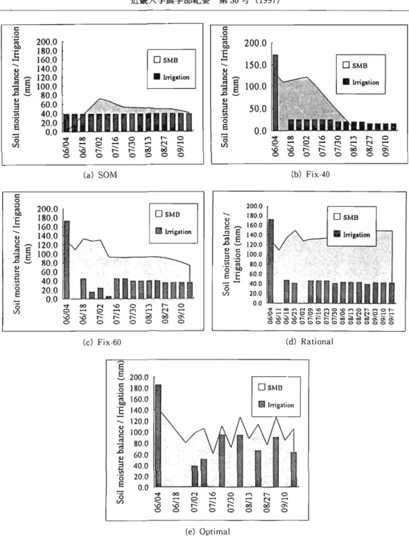
(15) 87. HATCIIO: Irrigation Water :Vlanagement through Information Management Table 2-3. Simulation results of different scheduling methods Method (unit) SOM Fix-40. Total supply. Irrigation loss. (over· irrigation). Net crop use. Efficiency. (m 3 ). (m'). (m'). (m 3 ). 15.482,880. 6,068,649. (377,245). 9,414.231. 61. 95. 5. 9,632,716. 3,496,012. (27,666). 6,136,704. 64. 69. 24. Possible damage. (%). Fix-60. 13,131,431. 4, 54,364. (127,026). 8,277,067. 63. 86. 9. Rat. 12.149,754. 4,378.993. (4.556). 7,770,761. 64. 72. 7. Opt. 13,090.945. 4,712,695. .378,250. 64. 82. 0. Irrigation loss: Sum of irrigatioll water 10. and distribution efficiencies,. assign d by the user by application. method, followed by Fix·60 method. It does not necessarily mean that 24% of paddy crop will be damaged for Fix-40 method, but all ponded water on the oil surface was consumed in 24% of an irrigated area, and it could reduce paddy yield. However, in case of paddy rice cultivation, any damage would not be registered until water retained in a soil is also depleted in addition to the ponded wal\:r on the field surface, Under plot-to-plot irrigation. the possibility is high that plots at the lower order of irrigation can not receive sufficient water for cultivating paddy, especially during the land preparation period. In fact, monthly analysis of irrigation performance revealed that the planned land preparation during June had to be postponed to mid July in sections with relatively large irrigated area. Opt method showed the best performance followed by SOM and Fix-50 or Rat methods. Irrigation application timing and weekly variations of ponded water depth by different scheduling methods are shown in Fig. 2-2. As it is shown in SOM «a) of Fig. 2-2), qual depth of water was applied every week and the depth of ponded water varied accordingly. However, the ponded water depth never reached to the required depth of land preparation. Some of plots within the :vn i-PL 1 10 was land prepared first by using allocated flow, while the other plots delayed land preparation until the discharge water from the upper fields flows into their plot. PL I 10 had sandy loam and the ponded water depth could reach to the maximum of 70 mm in early July, but sub-groups with loam and clay reached to the average ponded water depth of 150 mm in the end and early July, n::;pectively. MU with sandy soil could not maintain the ponded water layer, and the water depth drnpped to 0 mm in the second week of July, which could lead to possible crop damage. Thus ~OM method could assure qual acc ss of wat r with respect to the size of holding, but could not reflect variation in water demands by soil types, which lead to on'r-irrigation or possible crop damage. In demand-oriented methods. except for Fix methods which u e a fixed volume of application, irrigation demand can be reflected in an application volume as long as it is within the supply limit. In I~ational method, an application depth corresponding to crop water requirements and deep percolation was to be applied. The planned irrigation volume was adjusted according to the limit of possible supply. In Optimal method, irrigation wa. cheduled when ponded water level became lower than the assigned depth, how ver, the timing of irrigation is not known beforehand. Optim<ll method might not be very practical to apply becau farmers can not know in advanCE' when and how much water they will receive. From the point of view of operating and managing an irrigation system. SOM is the easiest whE'n a proportional flow division structure is available. Once an incoming flow is determined, the flow can be distributed proportionat Iy according to the command area of each intake gates. Thu~, the method would be suitable where no variations in waleT demands are expected..
(16) Jlifl*$&:!$$*C~. 88 c .Sl. C>l). ]. ;. ";;l .J:J U. = '" 0. ~. 8. m30~ (997). I. 3. Vi. '0. e. '0. ',lj. 200.0 180.0 160.0 140.0 120.0 100.0 80.0 60.0 40.0 20.0 0.0. OSMB. ....... 150.0. 1:$. .1Irig.tion. ~~. ~. ";;l. OSMB. •. 100.0. lnig.tion. .J:J~. ~ e. 50.0. III. '0 ~. Vl. 200.0. C>l). ]. N. 00 ...... ~. \l). ;a. 0. 0. ~. r0. 0. ..... ...... r\l). ~. r0. 0. ...,...... ::: ...... 0\. r-. N ...... oo. 00 0. 0. 0.0. '0. ~. ~. Vl. ~. 0. ...... 00. ;a 0. ~. ..... ....... 0. 0. 0. 0. N. r-. \l). r-. ~. r-. ..., ..... ...... oo 0. r-. 0 ...... ~. Q;. 0. 0. 00. (b) Fix·40. (a) SOM c 0. '.l:l. '"tlIl. ]. ...... u. u. ;~. (;l. ~. .J:J~. u. 2 III. 0. E. '0 VJ. 200.0 180.0 160.0 140.0 120.0 100.0 80.0 60.0 40.0 20.0 0.0. 200.0 180.0 OJ u c ~ 160.0 '" E 140.0 ~ E .J:J~ 120.0 ~ c: 100.0 3 .~ ~ 80.0 60.0 E ..... 40.0 '0 VJ 20.0 0.0. ....... OSMO. ml. lnigation. OSMB. .g. v. 0. ...... \l). -. J.dJUWm ..., ...,. 0. 00. :::::: \l) 0. N. ~. r-. 0. \l) ..... ...... r-. 0. r-. 0 ..... ...... ...... r- oo 0. S ....... N ...... 00. ~=~(;g~~E(3:g~oI'8~~. ~\D\D\D;::t:;t::t-"t--oo~SS~O\O; 0000000000000000. 0\ 0. 0. 0. 'E. (d) Rational. (c) Fix-60. I c. 0 '.l:l. '" ]. C>l). 8 :;j. ";;l .J:J. u. 2 III. '0 E '0 VJ. 200.0 180.0 160.0 140.0 120.0 100.0 80.0 60.0 40.0 20.0 0.0. OSMO. rtillmg31ion. !2 \l). v. ..... ...... \l). 0. 0. 00. N. !2 r0. \l). ...... r0. ..., ...... r0. 0. ...,. ..... ...... oo 0. (e) Optimal Fig. 2 -2.. Weekly variations of ponded water depth by different scheduling methods. However, farmers under the same MU should establish good water allocation rules, otherwise there is a high risk of water being monopolized by upstream users. In addition, the use of SOM under the current system setup (equal intake capacity) would cause a shortage in sections with large command areas and a loss in those with small command areas. If the installation of a.
(17) HATL'IIO:. (c) RIll. Irrigation Water Management through Information lVtanagement . a - I Os-rJ O .... J. 1'00 11001---, ii1llOOf-_ _, ~IOO. ::. ~ ,Ill). o~ ~ ~ ~ i ~ i ~ ~ i i ~ ~ ~ ~ ~ Fig. 2-3.. Operation Requirements of Main Canal on a daily basis. proportional division structure is not feasible, the size of command area should be adjusted by increasing the number of intake gates when command area under one intake gate is relatively large. In demand-oriented methods, frequent adjustment of check gate in the main canal would be necessary to achieve the performance shown in Table 2-3. Fig. 2-3 shows gate adjustment requirements of different scheduling methods under three sectors. Large fluctuations were observed for OPT and I~A T methods. To minimize the operation requirements and achieve better performance, simulation results can be used to operate check gates and flow allocations. Check gates can be operated on a weekly basis and maximum or mean flow shown in Fig. 2-3 in one week duration can be used as the actual operation flow for the entire week so that a daily gate adjustment would not be required. For example, the main canal flow during September 11 ~ 18 can be cut to 1,000 lis instead of adjusting a flow on a daily basis. This type of operational adjustment could be introduced easily by knowing how water should be controlled at each operating points. It was found that under paddy cultivation with homugeneous field conditions the application of SOM or Fix method which does not necessarily reflect crop water demands can be a viable scheduling method, because the ponded water on the field surface can work as a buffer against the short-term shortage or excess of water.. Conclusion. Water management practices of two different irrigation systems have been simulated and analyzed by applying the irrigation scheduling module of SIMIS. In the application in Argentina, new option of irrigation scheduling based on a supply-oriented approach has been added to simulate ongoing management practice. It has been made clear that current management practice based on a supply·oriented approach involves large water losses, because the water allocation is based on water rights and the supply c10es not reflect the actual crop water demands. Tu alleviate the problem of supply-oriented approach of water distribution, scheduling methods based on a demand-oriented approach have been used for the same tertiary unit. Scheduling methods based on CWR or S:YIB could save as much as 50% of wakr supply compared with a supply-oriented approach. However, the demand·oriented approach poses problems from the point of view of practical canal operation, because flow variations in the tertiary canals are high. Five additional simulations have been carried out to better adapt the method to practical management practice by introducing supply adjustment factors and rotational irrigation. The. 89.
(18) 90 results were very encouraging, further reducing the supply volume and improving the operational constraints caused by varying flow in tertiamy canals. In Thailand, the program was tested for its applicability under paddy cultivation condition, which has a distinct irrigation practice comrared to upland crops, especially during land preparation period. Under upland crop cultivation, the shortage or the excess of water supply could directly lead to crop damage or water loss. However, in paddy fields the ponded water layer on the surface could work as a buffer against the limited supply, and minimize the impact of water shortage. Lowered water layer can be recovered when the supply becomes abundant or with big rainfall. When the irrigation is determined by crop water requirements, relatively larger area can be irrigated under paddy growing condition compared to upland crops because of water storage function of paddy fields. As has been discussed. irrigation performance can be different by adopting different scheduling approaches. It can not be improved only by operational measures, but associated infrastructural improvements are required. To determine which scheduling method to introduce to a specific irrigation system, local specific conditions such as the cost of labor and infrastructural setups, the capacity of staff to manage the system, and the value of water should be taken into account. From the point of view of designing an irrigation system, more attention should be paid to how the system would be managed and operated. Irrigation scheduling module of SIMIS is very flexible to cope with variations of management practices and infrastructural setup. Analyses of system performance by SlyllS can provide useful guidelines of how the system should be improved in terms of infrastructure and management practice. It has been made clear that scheduling options available in the software can be an efficient tool to establish locally adapted water management practices which could save water and avoid crop damages. Application will not be limited to operation purposes. SIl'vllS could be used to design an irrigation system to know how the system could be operated under specific infrastructural setup so that a mismatch betwe n infrastructure and operation and management practice can be minimized. In addition, the astablishment of information system will open a way to use more advanced computer system for management purpose such as GIS (geographic information system).. References 1). 2) 3) 4) 5) 6) 7). N. HATCIlO and ].A. GARDOY: Computerized Irrigation Management Information System. Proceedings of the International Workshop on the Application of Mathematical Modeling for the Improvement of Irrigation Canal Operation. pp.121 129. CEMAGREF-IIMI. (1992). K HATcllo: Journal of JSIDRE. 63(4),31-36 (1995). FAO: CLlMW AT for CROP'" AT-A Climatic Database for Irrigation Planning and :Vlanagement. Irrigation and Drainage Paper 49. FAO, RO:VIE.(1993). FAO: Applications of Climatic Data for Effective Irrigation Planning and Management. Training Manual. pp.49-52. FAO. Rome.(J990). FAO: Crop Water Requirements (revised). Irrigation and Drainage Paper 24. FAO, Rome. (l979) . FAO: Yield Response to Water. Irrigation and Drainage Paper 33. pp. :n-57. FAO, Rome. (1992). L. SIIA:--;!\l\ : An International Journal of Agricultural Water Management. 22 (l), 97-102 (l992) ..
(19) HATCl t O:I r r ] gat i onWat erManagemet nt hr oughI no fr mat i onManagemet n. 91. 情報管理 による潅概水管理 八丁信正. 要. 約. 較検討 を行 った。 これによ り畑作の場合,水供給 の. 潅概 システムの管理 においては. システムの管理. 変動が直接的に作物 の収流や水分 ロスにつなが るも. に関する怖報が収躯 されているに もかかわ らず,惜. のの,水田単作の場合,水供給 の変動の影響 が畑作. 報処理能力の不足あるいは処理 システムの未整備の. の場合 ほ ど大 き くない とい うとこが明 らか にな っ. ため,有効な活用が行われていない場合が多 く見 ら. た。 これは,水稲単作 の場合,水田袈面の湛水が供. れ る。竹報 を有効 に処理 し,統合的に管理す るシス. 給の変肋に対する調整横能 を持 っているため,供給. テムが構築で きれば,潅概の水配分 を含む多 くの管. の変動 を吸収 して安定化 させ る効果のあるためであ. 理局面において有効 な判断が下せ るもの と期待 され. ると考 えられ る。. るO そこで,沼野主可塑の管理 をお こない効率的な. SI MI Sを導入す る耕 によ り,潅概管理 の改藩のた. 輔要 と供給 のバランス調整 を行 うことを目的 として. めの各種 の代替案について,突際に現地 に適用する. SMI I S( 潅概I J l 菓情報管理 システム) を開発 した。 I Sを,アルゼンチン及びタイ という大 き この SMI. る収血への影・ W な どについて比較検討する郡が可能. ことな く,水の供給必要丑,潅概 ロス,水不足 によ. く適 う潅概 システムに適用 し, その機能,実用性 に. となった。 また,各団場毎の取水時間 を明確 に決定. ついて検証 を行 うとともに,地域の特性 に対応 した. す る耳目こよ り水路上流部での過大な取水 を防止 し,. システムの改醤 ・変更 を行 った。 アルゼンチンにお. 平等な水配分 を行 う串が可能である。 さらに,多 く. いては,乾燥地域 の多様 な畑作物が栽培 され る潅概. の潅概 スケジュールオプションを用忠 してお り,多. システムに対す るシステムの適用 を行 い,現在行わ. 様 な確概 システムの管理 に柔軟 に対応可能である。. れている供給主導型 の水管理 と,群要主導型の水管. 液概 システムの運用効率 の改沓 ためには, こうし. 理 を番人 した場合の比較検討 を行 った。 その中で,. たシステムの導入 は,第 1段階にす ぎない。管理ny '. それぞれの管理手法による問題点,改沓点 を明 らか. 佳肴 は管理す るシステムの問題点 ・改沓すべ き点に. にするJ Jl が出来た。. ついて十分理解 してお く必要がある。 さらに, シス. タイでの適用にあたっては,水稲単作 とい う条件. テムの運用に必要な情報 の収媒 ・伝達 システムの改. 下で,新 たに水稲作での水管理 ( 特 にシロカキ期). 馨が必要であ り, それ を行 う職月への訓練 もI E勢で. MI Sに含 まれ のための計許 オプシ ョンを追加 し,SI. ある。. る 4つの液概 スケジュール方法の有効性 について比.
(20)
図

+7


関連したドキュメント
Answering a question of de la Harpe and Bridson in the Kourovka Notebook, we build the explicit embeddings of the additive group of rational numbers Q in a finitely generated group
The variational constant formula plays an important role in the study of the stability, existence of bounded solutions and the asymptotic behavior of non linear ordinary
Then it follows immediately from a suitable version of “Hensel’s Lemma” [cf., e.g., the argument of [4], Lemma 2.1] that S may be obtained, as the notation suggests, as the m A
Definition An embeddable tiled surface is a tiled surface which is actually achieved as the graph of singular leaves of some embedded orientable surface with closed braid
We give a Dehn–Nielsen type theorem for the homology cobordism group of homol- ogy cylinders by considering its action on the acyclic closure, which was defined by Levine in [12]
In order to be able to apply the Cartan–K¨ ahler theorem to prove existence of solutions in the real-analytic category, one needs a stronger result than Proposition 2.3; one needs
Zhang; Blow-up of solutions to the periodic modified Camassa-Holm equation with varying linear dispersion, Discrete Contin. Wang; Blow-up of solutions to the periodic
Kartsatos, The existence of bounded solutions on the real line of perturbed non- linear evolution equations in general Banach spaces, Nonlinear Anal.. Kreulich, Eberlein weak
