INVITED PAPER
Special Section on Leading-Edge Applications and Fundamentals of Superconducting Sensors and DetectorsSQUID Systems for Geophysical Time Domain Electromagnetics (TEM) at IPHT Jena
Andreas CHWALA†a), Ronny STOLZ†, Matthias SCHMELZ†, Vyacheslav ZAKOSARENKO††, Matthias MEYER††,andHans-Georg MEYER†,Nonmembers
SUMMARY Forty years after the first application of Superconducting Quantum Interference Devices (SQUIDs) [1], [2] for geophysical purposes, they have recently become a valued tool for mineral exploration. One of the most common applications is time domain (or transient) electromag- netics (TEM), an active method, where the inductive response from the ground to a changing current (mostly rectangular) in a loop on the surface is measured. After the current in the transmitter coil is switched, eddy cur- rents are excited in the ground, which decay in a manner dependent on the conductivity of the underlying geologic structure. The resulting secondary magnetic field at the surface is measured during the off-time by a receiver coil (induced voltage) or by a magnetometer (e.g. SQUID or fluxgate).
The recorded transient signal quality is improved by stacking positive and negative decays.
Alternatively, the TEM results can be inverted and give the elec- tric conductivity of the ground over depth. Since SQUIDs measure the magnetic field with high sensitivity and a constant frequency transfer func- tion, they show a superior performance compared to conventional induction coils, especially in the presence of strong conductors.
As the primary field, and especially its slew rate, are quite large, SQUID systems need to have a large slew rate and dynamic range. Any flux jump would make the use of standard stacking algorithms impossible.
IPHT and Supracon are developing and producing SQUID systems based on low temperature superconductors (LTS, in our case niobium), which are now state-of-the-art. Due to the large demand, we are addition- ally supplying systems with high temperature superconductors (HTS, in our case YBCO). While the low temperature SQUID systems have a better performance (noise and slew rate), the high temperature SQUID systems are easier to handle in the field.
The superior performance of SQUIDs compared to induction coils is the most important factor for the detection of good conductors at large depth or ore bodies underneath conductive overburden.
key words: SQUID, magnetometer, geophysical exploration, time domain electromagnetics
1. Introduction
In the past, many deposits have been found by geological sampling or geochemical methods, as outcrop or traces from the deposit could often be found at the surface. Nowadays, most of these ore bodies have already been exploited and ex- ploration teams need to rely more on geophysical methods.
However, at the same time geophysical exploration is be- coming more difficult as the targets are at larger depth. For electromagnetic methods an additional difficulty can be con-
Manuscript received June 30, 2014.
Manuscript revised September 25, 2014.
†The authors are with Leibniz-Institute of Photonic Technol- ogy, A Einstein Str 9, 07745 Jena, Germany.
††The authors are with Supracon AG, An der Lehmgrube 11, 07751 Jena, Germany.
a) E-mail: [email protected] DOI: 10.1587/transele.E98.C.167
ductive overburden: most of the signal is generated from a conductive layer on top of the deposit. Thus, sensitive tools and sophisticated inversion techniques become necessary.
One important method in mineral exploration is Time Domain Electromagnetics (TEM), which will be explained in more detail in the next chapter. Different groups around the world have developed geophysical SQUID receiver sys- tems for TEM [3]–[6]. They benefit from some of the spe- cial characteristics of SQUIDs: a constant response over the whole frequency range, the direct measurement of the mag- netic field, and their high sensitivity.
While all other systems are based on high temperature superconductors, in 1999 IPHT started to develop SQUIDs for geophysical applications with our proprietary niobium technology. The development of the HTS SQUID systems (at IPHT already started in 1995) was on hold, but was started again after the successful commercialization (driven by Supracon AG) of the LTS SQUID systems in 2004.
2. The TEM Method
TEM works in the time domain, in contrast to other methods (like AMT, MT, CSAMT) operating in the frequency do- main. The abbreviation TEM also stands for transient elec- tromagnetics as it measures the magnetic or induced tran- sient voltage caused by a transient current in the transmitter loop, which is a measure of conductive bodies in the sur- roundings.
The typical TEM layout is a square transmitter (TX) coil with 100 to 400 m side length with the TX generator placed at one corner, outside the loop. The receiver (RX, in- duction coil or magnetometer) is stably placed in the center of the TX coil (moving loop configuration). In order to map the area the loop and the receiver are moved together along profile lines. Larger TX loops are typically kept stationary for most of the time (fixed loop configuration), at a position where optimum coupling to the target is expected and the receiver is moved along profile lines. While in the first con- figuration, profile plots of the measured signal directly vi- sualize changes of the conductivity in the ground, the latter one needs a correction for the primary field strength along the profile. The moving loop configuration is in any case preferred as the coupling of the primary field to any target will certainly happen at some point, while the fixed loop configuration needs some a priori information as to where to place the loop.
Copyright c⃝2015 The Institute of Electronics, Information and Communication Engineers
Fig. 1 Schematic of a typical TEM setup with a SQUID magnetometer triple.
Transmitter loop size and current are adjusted accord- ing to the problem—for deep lying targets one would use large TX coils together with a larger current to produce a strong dipole moment. For shallow objects in resistive ter- rain, loops need to be smaller and the current possibly lower as the early time response gets very important, which means the TX should switch off very fast which is only possible with small inductances/loop sizes.
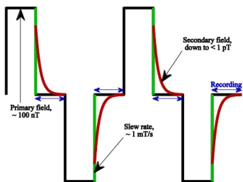
A receiver (RX), which needs to be exactly synchro- nized to the transmitter current, records the transient re- sponse as shown in Fig. 2 after the current in the TX loop is switched off.
By averaging, called stacking, the response of the 2 po- larities of the TX static offsets at the receiver (input ampli- fiers, filters) and the sensor are suppressed. Furthermore, many of these cycles are stacked in order to lower the noise influence. A simple averaging is most useful for white noise;
more sophisticated stacking algorithms (e.g. tapered stack- ing [7]) can also suppress drifts. But none of the currently applied stacking algorithms can cope with abrupt changes in the offset voltages that would occur if the SQUID experi- ences flux jumps during the measurement.
In case of measuring with coils, several hundreds or even thousands of cycles are stacked, which can be very time consuming. One of the big advantages of SQUID systems is the need for much less stacks due to the lower noise level [8].
Another big advantage of SQUIDs is the direct mea- surement of the magnetic field, as will be shown in the next paragraphs. For example, the B-field over a conductive half space decays with [9]
Bh=Aht−32, (1)
while the induced voltage in a coil, the time derivative of (1), will decay much faster:
Uh=−dΦ dt =−3
2AAht−52. (2)
For an ore body with certain conductivity the B-field decays with [9]
Fig. 2 Timing of TX signal (primary field) and the recorded transient response (secondary field) in a TEM measurement.
Bc=Ace−tτ, (3)
which translates for the induced voltage to Uc=−dΦ
dt =−AAc
τ e−τt. (4)
Here,AhandAcare scaling factors;Ais the area of the RX loop.
For the comparison of the two sensor configurations let us assume the simple case of a good confined conductor in a much less conductive host material with homogenous conductivity. By summing up (1) and (3) or (2) and (4), respectively, we get the following decays for the B-field and the induced voltage:
B=Bh+Bc=Aht−32 +Ace−τt. (5)
U=Uh+Uc=−3
2AAht−52−AAc
τ e−τt. (6) A simulated response using this approach is depicted in Fig. 3 for a time constant ofτ200 ms (in order to plot BandUinto the same graph A is assumed to be 10−3m2).
Full lines visualize the measured signal, while the dashed lines correspond to the half space response and the dotted lines represent the response of the ore body. The vertical (red) lines mark the time where the signal measured is 30%
larger than the signal of the half space (in logarithmic units), in this case 41 ms for the magnetic field sensor compared to 153 ms for the coil. This means, that a conductor can be recognized about 3 times earlier for a B-field measurement, which leads to a drastic reduction in the necessary number of stacks or for the same number of stacks to a much cleaner signal.
In order to draw a readable graph, we have assumed that the signal from the conductive ore bodyAcis 1000 times larger than that for the host material, which is the half space responseAh. The ratio would be similar for other situations as well, but the contrast would be much smaller in both cases if the signal from the conductor is weaker—making the di- rect B-field-measurement even more important.
Fig. 3 Comparison of the signal, as measured by TEM via a B-field- sensor and a coil (U).
3. Requirements for SQUID Systems
From the method described in chapter 2 we can derive sev- eral requirements for SQUID systems (values in brackets as an example for 10 A in a 100×100 m2loop):
1. high dynamic range to cope with a large primary field (113 nT at the center of the loop),
2. high slew rate to withstand fast transients (113 nT in typically 100µs→1.13 mT/s),
3. step response as fast as possible in order to detect a clean early time secondary field,
4. use of materials without any response to the pri- mary field (no magnetic hysteresis or eddy cur- rents).
All these requirements should impair the noise perfor- mance of the SQUID sensor as little as possible. There- fore, developing fast, low noise, low drift and stable feed- back electronics is one of the primary tasks in the system development.
A thorough optimization of the flux locked loop (FLL) feedback circuitry is mandatory for a fast (large bandwidth and high slew rate) yet stable SQUID system. As said be- fore: every flux jump would make the stacking in the TEM impossible and this probability must be minimized.
A SQUID system should at least measure the vertical magnetic field, since this is usually the component with the largest signal (and lowest geomagnetic noise). However, very often the horizontal components are also of interest, es- pecially for a more detailed modelling and inversion. Hence, a SQUID system should measure a set of three orthogonal components, which we shall call here a triplet. It is impor- tant to have the orientation accurately shown and labelled outside of the cryostat. A level should be mounted on top in order to vertically align the system properly.
As the instruments will be used under harsh conditions, special attention must be paid to mechanical stability, work-
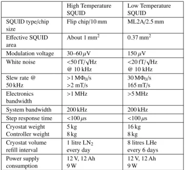
Table 1 Typical parameters for HTS and LTS SQUID systems.
High Temperature SQUID
Low Temperature SQUID SQUID type/chip
size
Flip chip/10 mm ML2A/2.5 mm Effective SQUID
area
About 1 mm2 0.37 mm2 Modulation voltage 30–60µV 150µV White noise <50 fT/√
Hz
@ 10 kHz
<20 fT/√ Hz
@ 10 kHz Slew rate @
50 kHz
>1 MΦ0/s
>2 mT/s
30 MΦ0/s 165 mT/s Electronics
bandwidth
>1 MHz >5 MHz
System bandwidth 200 kHz 200 kHz
Step response time <100µs <100µs Cryostat weight
Controller weight
5 kg 8 kg
16 kg 8 kg Cryostat volume
refill interval
1 litre LN2
every day
8 litres LHe every 6 days Power supply
consumption
12 V, 12 Ah 9 W
12 V, 12 Ah 9 W
ing and storage temperatures (e.g. cables and rubber in seal- ings) and robust cryogenic equipment. Power consumption should be minimized as the batteries need to last a full work- ing day, even at sub-arctic temperatures down to−40◦C.
In all probability, the potential user will already own a TEM system (TX generator with clock control that is syn- chronized to a RX data acquisition system); the SQUID in- terface should be able to connect to any of these receivers.
In order to avoid grounding problems, which could again produce noise, a symmetric, low impedance output should be implemented.
4. System Setup
Table 1 lists the typical parameters of both kinds of our SQUID systems developed at IPHT. Please note that the HTS SQUID parameters are not as reproducible as the LTS SQUIDs due to the fabrication process explained below.
The cryostats from Cryoton, Russia, are made from re- inforced fiber glass in order to minimize any response to the primary field. The superinsulation is installed in such a way that conductive paths are minimized. The liquid he- lium cryostat (8 l liquid volume) has a holding time of 6 days, whereas for the HTS SQUID system the volume for liquid nitrogen cryostat is much smaller (1 l) so the refilling (every day) is easier and faster. The RF shield, made of alu- minum foil is mounted directly outside on the cryostat and is protected by a bucket (the weights in Table 1 are including electronics and bucket).
Power is supplied by built-in service-free lead batter- ies. The capacity has been adjusted in such a way that the systems can be operated for about 8 h at−40◦C, which cor- responds to 16 h operation at 20◦C.
Due to the small dimensions of the nitrogen cryostats a directly coupled integrated SQUID electronics, capable to operate with dc and ac bias, was developed [10] with a foot-
print of only 18 mm by 47 mm. We could, at that time, only implement a single integrator feedback due to the limited space—which cannot achieve the slew rate of more sophis- ticated FLL electronics [11].
All SQUIDs are fabricated in the IPHT clean room.
The LTS SQUIDs are based on sub-µm Josephson junctions and are fully integrated with an inductively coupled multi- loop antenna [12].
In order to improve the yield, the HTS SQUIDs and its antenna are produced separately and mounted face-to- face in a flip chip technique [13]. The HTS SQUIDs are single layer washer SQUIDs, YBaCuO films deposited on 30◦bi-crystal STO substrates by laser ablation. 11 SQUIDs are aligned along the grain boundary; the critical current and resistance vary typically by 30% while the modulation voltage can vary from 10 to 60µV. The best SQUID is se- lected for the flip chip. The antenna with a pick-up area of 7.6×7.6 mm2 is produced on STO substrates in a 3 layer process; the inductive coupling to the SQUID washer is im- plemented by a 15 turn on-chip input coil.
We report here on the latest developments on LTS and HTS SQUID systems as there are now four development generations in both branches. It should be noted that the latest LTS SQUID system [14] features 2 sets of SQUID triplets; Table 1 only lists parameters for the low sensitivity SQUIDs which are intended for TEM measurements. The additional triplet of high sensitive SQUIDs (<2 fT/√
Hz) is designed for the use in geophysical methods with weak sig- nals (LOTEM, CSAMT) or even passive (MT, AMT).
5. Performance in the Laboratory and in the Field A very important step, before bringing any device into the field, is its careful optimization and characterization in the laboratory, which will be explained in the subsequent para- graphs. These tests are followed by application-like tests in the field, described thereafter.
For the characterization of intrinsic SQUID parameters we use combinations of Cryoperm [15] and superconductive shields. Different sets of magnetic shielding cans are avail- able for the noise measurement of the cryostat. The whole system can also be placed in a magnetically shielded room (2 layers of MUMETALL, 1 layer aluminum [15]) to deter- mine the overall performance and the stability in the absence of high and most of the low frequency interferences, since the construction and the aluminum frame provide a good ra- dio frequency (RF) shield.
Both options are only useful to quantify the white noise level of the systems, as the magnetic shielding is not good enough at low frequencies (and the external noise at low frequencies is higher as well).
Noise spectra are calculated from recorded time series using National Instruments 4461 boards with 24 bit resolu- tion and up to 200 kHz sampling rate in a PXI rack.
Figure 4 shows the noise spectrum of a LTS SQUID system (low sensitivity triplet) in a 4-layer-shield cylinder in our lab, while Fig. 5 shows the noise of the same system
in our shielded room. For comparison, the noise of a HTS SQUID system with ac bias in the shielded room is given in Fig. 6. The low frequency noise is in all cases dominated by signals from the surrounding environment with disturbances from, for example, elevators or doors opening or closing.
The rest of the spectra is mostly dominated by 50 Hz and harmonics.
As the measured system noise in a magnetically shielded environment may not reflect the one as in the pres- ence of the Earth’s magnetic field, it would be preferable to measure the system noise under real application conditions i.e. in the field. These measurements should be carried out in a rural area with two identical systems; the intrinsic noise can in this case be calculated by correlation techniques [14].
The same method cannot be used in the shielded room, be- cause the signals at both cryostat locations are very different due to field gradients in the shielded room.
In order to calculate the magnetic field noise spectra the system has to be calibrated first. Helmholtz coils [16] are used for the measurement of the transfer function (Voltage output as a function of the applied magnetic field and its
Fig. 4 Magnetic field noise spectrum of an LTS SQUID system in a shielded cylinder (4 layers).
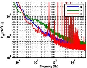
Fig. 5 Magnetic field noise spectrum of an LTS SQUID system in the shielded room at IPHT.
Fig. 6 Magnetic field noise spectrum of an HTS SQUID system with ac- bias in the shielded room.
Fig. 7 Typical magnetic field noise spectrum of LTS SQUID system from a field test close to Jena.
frequency) and the orthogonality of the SQUIDs.
A very important part of the system is the RF shield around the cryostat, which prevents signals from penetrating through to the SQUID and causing flux jumps. On the other hand, it should have a very fast step response that should be no longer than 100µs. The shield consists mainly of alu- minum foil. The thickness of the foil is of the order of sev- eral 100 nm (also depending on the geometry) so as to have low pass characteristics in the range of several 100 kHz. Dif- ferent sets of coils and RF probes are used together with network analyzers in order to optimize the RF screen. Each system is checked with different types of irradiation—the users around the world are exposed to quite a variety of RF sources, ranging from masts with cell phone installations to radars from airports to pulsed transmissions from digital TV broadcasts.
Finally, after all optimizations, the system stability is determined in the shielded room by recording time series with a sampling rate of 1 kHz for several hours. This step is necessary especially for high temperature SQUIDs as some individual sensors show too many flux jumps for, up to now,
Fig. 8 System response of the LTS SQUID system to a 20µs transient;
samples at 10µs intervals.
unknown reasons.
Additionally, each system is further tested in the field before it is released for the use by customers. This involves recording the noise in a place several kilometers outside of the town Jena and carrying out a complete TEM measure- ment. Figure 7 shows a typical noise spectrum of the LTS SQUID in the field. With a sufficiently high sampling rate one can at least determine the white noise of the system in the excitation gap of the Earth’s magnetic field between 1 and 10 kHz [7]. The recorded noise is again strongly dom- inated by external sources: 50 Hz and harmonics due to power lines, 16 2/3 Hz from railway and strong low fre- quency noise e.g. by cable car.
Another important test is to determine the system re- sponse: a small loop (diameter about 1 m) is placed at a distance of several meters from the system and a fast TEM current transient, faster than the typical 100µs switch off, is applied. Current and distance are adjusted in order to achieve a typical amplitude at the SQUID on the order of 100 nT. As the loop is very small, there will be no response from the ground: The recorded transient from the SQUID system shows the system response and should decay as fast as possible. An additional inductance in series with the loop is used to slow down the switch offin order to meet slew rate requirements of the SQUID system.
A typical measured system response of the LTS SQUID system is depicted in Fig. 8. The sampling rate of 100 kHz results in 10µs interval between the samples. The current in the transmitter was switched offin 20µs. The switch- offtime was measured with an oscilloscope at a resistor in series to the TX loop. For clarity the polarity of channel x in this plot is reversed (the primary field seen by the horizontal components x and y depends on the geometry of the setup between the small loop and the cryostat). It can be observed, that the system response is faster than 60µs. The peak at about 40µs has not investigated further as the performance is sufficient for all standard TEM measurements in the target depth and conductivity range. In all probability the response of the system is even faster.
Fig. 9 TEM signal over a good conductor for a LTS SQUID and a coil.
Please note the logarithmic scale, while the scale between−10 m and 10 m is linear.
Fig. 10 TEM signal as in Fig. 9, but the SQUID signal is differentiated over time.
6. TEM Measurements
In order to illustrate the performance of an LTS SQUID in comparison with an induction coil (surface PEM receiver coil from Crone with built-in amplifier and an effective area of 4000 m2), Fig. 9 depicts a measurement carried out with the LTS SQUID in northern Germany. The TEM transient has been recorded up to one second, two repetitions with 256 stacks each are displayed. The TX was a Crone 2.4 kW transmitter, switching about 10 amps into a 100 m×100 m loop; the switch offtime was set to 500µs. The receiver is a Crone P.E.M. receiver. A typical decay over this rather good conductor is given in Fig. 9. While the Crone coil signal gets noisy after 50 ms the SQUID signal is very clean up to 1 s. Both measurements compare very well up to 50 ms, as shown by differentiating the SQUID signal over time in Fig. 10. Of course the SQUID signal gets a little bit noisier by the differentiation, but would still be usable up to one second.
The target is, in this case, not a real ore body, but the
so-called North German conductive anomaly [17] which is a good conductor at a depth of about 300 m.
Conclusions
There are many geophysical exploration surveys that have shown the successful application of SQUIDs in TEM. How- ever, due to commercial constraints only a few examples have been published, a notable example is found in [8]. Cur- rently, there are about 15 of our SQUID system in use for TEM. Exciting new developments are currently conducted towards new electromagnetic methods in geosciences with SQUIDs and will increase their impact even further.
Acknowledgments
The authors are thankful to AngloAmerican, Discovery Geophysics, Lundin Mining, Crone Geophysics and Explo- ration, Geoterrex, metronix, TU Berlin and LIAG Hannover for their help and collaboration in many different SQUID projects. We also thank all our co-workers at IPHT and Supracon who have contributed to the development and ser- vice of the systems.
References
[1] R. L. Forgacs and A. Warnick, “Digital-analog magnetometer uti- lizing superconducting Sensor,” Rev. Sci. Instrum., vol.38, no.2, pp.214–220, Feb. 1967.
[2] J. E. Zimmerman and W. H. Campbell, “Test of cryogenic SQUID for geomagnetic field measurements,” Geophysics, vol.40, no.2, pp.269–284, Apr. 1975.
[3] K. E. Leslie, R. A. Binks, S. K. H. Lam, P. A. Sullivan, D. L. Tilbrook, R. G. Thorn, and C. P. Foley, “Application of high-temperature superconductor SQUIDs for ground-based TEM,”
Leading Edge (Tulsa Okla.), vol.27, no.1, pp.70–74, Jan. 2008.
[4] A. Chwala, J. P. Smit, R. Stolz, V. Zakosarenko, M. Schmelz, L.
Fritzsch, F. Bauer, M. Starkloff, and H.-G. Meyer, “Low tempera- ture SQUID magnetometer systems for geophysical exploration with transient electromagnetics,” Supercond. Sci. Technol., vol.24, no.12, pp.125006, Dec. 2011.
[5] M. Bick, G. Panaitov, N. Wolters, Y. Zhang, H. Bousack, A. I. Bra- ginski, U. Kalberkamp, H. Burkhardt, and U. Matzander, “A HTS rf SQUID vector magnetometer for geophysical exploration,” IEEE Trans. Appl. Supercond., vol.9, no.2, pp.3780–3785, June 1999.
[6] T. Hato, A. Tsukamoto, S. Adachi, Y. Oshikubo, H. Watanabe, H. Ishikawa, M. Sugisaki, E. Arai, and K. Tanabe, “Development of HTS-SQUID magnetometer system with high slew rate for ex- ploration of mineral resources,” Supercond. Sci. Technol., vol.26, no.11, pp.115003, Nov. 2013.
[7] J. C. Macnae, Y. Lamontagne, and G. F. West, “Noise processing techniques for time-domain EM systems,” Geophysics, vol.49, no.7, pp.934–948, July 1984.
[8] J. Macnae and T. LeRoux, “SQUID sensors for EM systems,” Pro- ceedings of Exploration 2007, Paper 25, pp. 417–423, 2007.
[9] S. H. Ward and G. W. Hohmann, “Electromagnetic theory for geo- physical applications,” in Electromagnetic Methods in Applied Geo- physics, Society of Exploration Geophysicists, ed. M. N. Nabighian, vol.1, pp.130–311, 1988.
[10] N. Oukhanski, V. Schultze, R. P. J. Ijsselsteijn, and H.-G. Meyer,
“High frequency ac bias for direct-coupled dc superconducting quantum interference device readout electronics,” Rev. Sci. Instrum., vol.74, no.12, pp.5189–5193, Dec. 2003.
[11] N. Oukhanski, R. Stolz, and H.-G. Meyer, “High slew rate, ultra- stable direct-coupled readout for dc superconducting quantum inter- ference devices,” Appl. Phys. Lett., vol.89, no.6, pp.063502, Aug.
2006.
[12] M. Schmelz, R. Stolz, V. Zakosarenko, T. Schönau, S. Anders, L.
Fritzsch, M. Mück, and H.-G. Meyer, “Field-stable SQUID mag- netometer with sub-fT Hz−1/2resolution based on sub-micrometer cross-type Josephson tunnel junctions,” Supercond. Sci. Technol., vol.24, no.6, pp.065009, June 2011.
[13] J. Ramos, A. Chwala, R. Isselsteijn, R. Stolz, V. Zakosarenko, V.
Schultze, H. E. Hoenig, H.-G. Meyer, J. Beyer, and D. Drung, “Low- noise Y-Ba-Cu-O flip-chip dc SQUID magnetometers,” IEEE Trans.
Appl. Supercond., vol.9, no.2, pp.3392–3395, June 1999.
[14] A. Chwala, J. Kingman, R. Stolz, M. Schmelz, V. Zakosarenko, S.
Linzen, F. Bauer, M. Starkloff, M. Meyer, and H.-G. Meyer, “Noise characterization of highly sensitive SQUID magnetometer systems in unshielded environments,” Supercond. Sci. Technol., vol.26, no.3, pp.035017, Mar. 2013.
[15] VACUUMSCHMELZE GmbH & Co. KG, Grüner Weg 37, D- 63450 Hanau.
[16] A. Chwala, F. Bauer, V. Schultze, R. Stolz, and H.-G. Meyer,
“Helmholtz coil systems for the characterization of SQUID sensor heads,” J. Phys. Conf. Ser., vol.1, no.158, pp.739–742, 1997.
[17] A. Schäfer, L. Houpt, H. Brasse, and N. Hoffmann, EMTESZ Work- ing Group, “The North German Conductivity Anomaly revisited,”
Geophys. J. Int., vol.187, no.1, pp.85–98, Oct. 2011.
Andreas Chwala studied physics at the Friedrich Schiller University in Jena, where he received his diploma in 1993. Since 1993 he is with the Institute for Physical High Technol- ogy (IPHT, now Leibniz Institute of Photonic Technology) in Jena. 1994 he started to develop and use SQUID systems for geophysical appli- cations, mainly TEM. He is also involved in the development and application of SQUID system for geomagnetic prospection, such as archaeom- etry and airborne exploration.
Dr. Ronny Stolz received his Ph.D. and State Doctorate degrees in physics in 1995 and in 2006 from the Friedrich Schiller University, Jena, Germany.
Since 1995 he joined the Department of Quan- tum detection of the IPHT in Jena and since 2007 he is head of the photonic magnetome- ter group. His research focuses are the devel- opment of superconducting electronics technol- ogy, SQUID sensors, high precision measure- ments and digital electronics. He is involved de- velopment of geophysical instruments using superconducting technologies like SQUID receivers for TEM and a full tensor magnetic gradiometer sys- tem for airborne exploration and archaeology.
Dr. Matthias Schmelz studied physics at the Friedrich Schiller University in Jena and re- ceived his diploma in 2007. After joining the IPHT in Jena in 2007 he is working on the devel- opment of SQUIDs based on cross-type Joseph- son junctions and SQUID systems. In 2014 he received his PhD from the University of Twente (The Netherlands).
Dr. Vyacheslav Zakosarenko received his master degree in electronics at the Moscow Institute for Physics and Technology (Dolgo- prudny). Between 1971 and 1976 he was re- searcher at Kapitza Institute for Physical Prob- lems (RAS) in Moscow where in 1981 he re- ceived Ph.D. degree in physics and mathemat- ics. He was with Lebedev Physical Institute (RAS) form 1976 to 1984 and then up to 1993 with Institute for Microelectronic Technology (RAS). From 1993 to 1996 he worked at in Friedrich Schiller University in Jena. Since 1996 he joined the IPHT in Jena. Currently he is with the Supracon AG in Jena. His expertise is in the experimental investigation of the superconductivity of thin films and devices on the base of Josephson junctions.
Matthias Meyer studied Intercultural Man- agement with a major in commercial infor- mation technologies at the Friedrich-Schiller- University Jena and the University of Edinburgh (United Kingdom). He received his diploma in the year 2000. After gathering work expe- rience at Ford Motor Company (London), IBM (Buenos Aires), Robert Bosch (Madrid) he went on to cofound the technology company Supra- con AG in 2001. Since then he has been in- volved in several joint research to develop in- dustrial applications for superconducting sensors.
Prof. Dr. Hans-Georg Meyer received his Ph.D. and State Doctorate degrees in physics in 1981 and in 1991 from the Friedrich Schiller University, Jena, Germany. In 1974 he joined the Department of Detector Physics at the Physics Division of the Friedrich Schiller Uni- versity, where he worked in the field of weak superconductivity, basically on dynamics of Josephson tunnel junctions. Since 1993 he is with the IPHT in Jena as the Head of the De- partment of Quantum Detection. Since 2010 he is professor for solid state physics at the Friedrich Schiller University. He has been involved in the development of superconductor electronics tech- nology and its application in precision measurement techniques, in partic- ular SQUID sensors and highly precise magnetic measurement techniques, and in detection of Infrared and Terahertz radiation.