Greenhouse Gas Inventory Accounting for Chinese Cities: A Preliminary Study

Chinese Cities: A Preliminary Study

著者 Ruixi Zhao, Yan Li

journal or

publication title

International Review for Spatial Planning and Sustainable Development

volume 4

number 4

page range 88‑104

year 2016‑10‑15

URL http://hdl.handle.net/2297/46725

doi: 10.14246/irspsd.4.4_88

88

DOI: http://dx.doi.org/10.14246/irspsd.4.4_88

Copyright@SPSD Press from 2010, SPSD Press, Kanazawa

Greenhouse Gas Inventory Accounting for Chinese Cities: A Preliminary Study

Ruixi Zhao

and Yan Li

*

1 Graduate School of Asia Pacific Studies, Ritsumeikan Asia Pacific University

*Corresponding Author: [email protected]

Received: August 04, 2015; Accepted: Dec 15, 2015

Key words: GHG inventory, Chinese cities, Beijing, GHG emission

Abstract: City Greenhouse Gas (GHG) inventory, a framework for measuring a city’s detailed emissions from all activities, provides scientific evidence for the purpose of policy-making. As one of the largest GHG emitters in the world, China aims to reduce CO2 emissions per unit of GDP to 60 to 65 percent below 2005 levels by 2030. However, city GHG inventories in China have not yet been published by the city governments. Furthermore, previous studies on city inventory accounting are neither complete nor globally comparable.

Hence, a case study of Beijing was conducted for the purpose of reporting the city inventory completely and enabling data to be comparable internationally.

This research quantifies Beijing’s latest emissions based on available data through multiple methods, including Community-Scale Greenhouse Gas emissions inventories (GPC), a method devised by the Japanese Ministry of Environment (Japanese Ministry of Environment, 2010) and a method from recent academic research on CO2 emissions in the Chinese iron and steel industry (Zhao, Y. Q., Li, & Li, 2012). According to these methods, Beijing’s GHG emissions were 373,558,617 t CO2 in 2012. Additionally, comparisons between Beijing and six other mega-cities of Shanghai, Tokyo, New York, Washington D.C., London and Paris show that Beijing’s 2012 GHG emission per capita and per 10,000 CNY GDP ranked the highest. This study creates a timely and relatively complete GHG emission inventory that can be widely applied for comparisons and presents recommendations for city inventory building.

1. INTRODUCTION

A city’s greenhouse gas (GHG) emission inventory, a framework for city governments to account for and report on urban GHG emissions data, estimates the quantity of GHG emissions associated with city sources and activities taking place during a chosen year (International Council for Local Environmental Initiatives (ICLEI), 2013). The GHG inventory is playing an essential role in mitigation, especially for assisting urban policy making, indicating the reduction outcomes and motivating urban actions. Currently, city inventories have been studied by a number of entities, including international organizations, governments and researchers worldwide.

According to the UN Intergovernmental Panel on Climate Change (IPCC)

(2006), GHG inventories shall calculate emissions of carbon dioxide (CO

),

methane (CH

), nitrous oxide (N

O), Hydro Fluoro Carbons (HFCs), Per

Fluoro Carbons (PFCs) and Sulphur Hexafluoride (SF

) with the following equation: GHG emissions= Activity data× Emission factor.

As one of the largest GHG emitters, China’s mitigation efforts attract global attention. As the capital, Beijing is the centre of this urgent concern.

However, a city inventory and CO

emissions are not publicized by the Beijing government and research on Beijing is facing the following series of issues: 1) most of the data are outdated because the latest emissions reporting calculated for Beijing, by Yuan and Gu (2011), took place in 2009; 2) accounting of gases was incomplete since only CO

emissions were calculated and neither forestry carbon sinks nor indirect emissions were covered; 3) studies were not globally comparable because most internationally recognized city inventories cannot be adopted. For instance, the study of Yuan and Gu (2011) shows that the International local government GHG emissions analysis protocol (IEAP) method is inapplicable for accounting Beijing’s emissions.

Initially, this research follows the Global Protocol for Community Scale Greenhouse Gas Emissions (GPC) framework, as it is the latest globally recognized city inventory method established by reputable inventory authorities including the United Nations Environmental Programme (UNEP), World Bank, World Resource Institute and ICLEI. Furthermore, the GPC’s framework has been adopted by 100 cities worldwide and even has a special version for Chinese cities (GPC, 2014). However, this study reveals that the GPC method can only cover 77% of Beijing’s 2012 GHG emissions. In order to compensate, this study refers to two additional methods – one from Japan, called the Manual of Planning against Global Warming for Local Governments (Japanese Ministry of Environment, 2010), and one academic paper from China used specifically for iron and steel production (Zhao, Y.

Q., Li, & Li, 2012).

This research aims to answer the following questions: What volume of GHG emissions did Beijing discharge in 2012, what issues have been found, and what relative improvements can be made? The calculation process follows four steps: 1) setting the geographical boundary and scope; 2) collecting activity data; 3) selecting factors; and 4) calculating emissions.

For the activity data, it will mainly be collected from the Beijing City Statistical Yearbook and Beijing City Environmental Protection Bureau’s reference documents.

2. GHG CITY INVENTORY

The GHG City inventory is playing an increasingly essential role for the

following reasons. First, the city inventory provides technological support

and references for setting mitigation goals and scenarios for both

government and individuals. Second, it assists cities in reporting GHG

emissions data and assessing emission reduction outcomes. Third, it is a

cornerstone for low-carbon city planning and helps to improve the quality of

low-carbon development. Moreover, development of an urban level

inventory also promotes the establishment and perfection of national level

inventory schemes. Finally, accounting processes and consequences of

emission inventories contribute to city comparisons and enhance

improvements for both domestic cities and international ones.

2.1 GHG Composition and Inventory Contents

According to the UN Intergovernmental Panel on Climate Change (IPCC) (2006), cities shall account for Greenhouse Gas emissions of six gases including carbon dioxide (CO

), methane (CH

), nitrous oxide (N

O), Hydro Fluoro Carbons (HFCs), Per Fluoro Carbons (PFCs) and Sulphur Hexafluoride (SF

). In detail, HFC includes HFC-23 , HFC-32 , HFC-125 , HFC-134a , HFC-143a, HFC-152a , HFC-227ea , HFC-236fa and HFC- 245fa, while CH

and C

F

are calculated in terms of PFCs. In 2012, Nitrogen Tri Flouride (NF

) was added to the second compliance period of the Kyoto Protocol, yet it has not been widely quantified since most of the well-used inventory protocols were released before 2012.

In general, GHG emissions are collected from different sectors and usually cover a 12 month period. A Japanese case is shown in the table below, wherein emissions are accounted from various sectors, and some sectors cover more than one type of gas. For instance, the transportation sector covers emissions of CO

, CH

and N

O. Table 1 provides a case of Oita Prefecture, which has similar calculation fields to those of Tokyo and is a prefecture in which the authors have performed emissions calculations in previous studies.

Table 1. Accounting Contents of GHG Inventory (a case of Oita Prefecture, Japan)

Sectors Calculated GHG

category

Fields

Energy Industry CO2

Manufacturing Industry

Agriculture, Forestry and Fisheries Construction and Mining

Residential CO2 Residential energy consumption

Commercial CO2

Commercial Sewage Waste Finance and Real Estate Public Service

Specified Business Operators Services Individual Services

Industrial Process:

cement

CO2 Cement

Transportation CO2, CH4 and N2O

Automobiles (CO2, CH4 andN2O)

Railway(CO₂); Shipping(CO₂); Aviation(CO₂)

Waste CO2, CH4 and N2O

Municipal Solid Waste Industrial Waste; Organic Waste Solid Waste Disposal on Land Water Treatment

Agriculture CH4 and N2O

Livestock breeding process Livestock waste Emission from paddy field Burning of crop residue Cultivation of organic soils

HFC, PFC,SF6 HFC, PFC, and SF6

Household refrigerator Air conditioners (automobile use) Specified business operators

Forestry CO2

Private Forests National Forests Source: Environmental Affairs Office of Oita Prefecture (2015)

2.2 City Inventory Methodology

Currently, there are a number of GHG inventory accounting methods that can be divided into two categories. The first category covers both direct and indirect emissions. Direct emissions are caused by citizens’ activities and are discharged within city geographical boundaries, while indirect emissions are also caused by citizens’ activities, but occur outside the city boundaries.

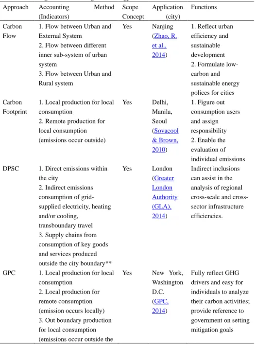
Carbon Flows (Zhao, R. et al., 2014), Carbon Footprint (Sovacool & Brown, 2010), DPSC (Greater London Authority (GLA), 2014) and GPC are included this category. Detailed descriptions are shown in Table 2. In the second category, only direct emissions are calculated. For instance, the UN Intergovernmental Panel on Climate Change (IPCC)’s framework, which is the first international standard for GHG inventory accounting, is included in this second category.

Table 2. Existing GHG accounting methodology Approach Accounting Method

(Indicators)

Scope Concept

Application (city)

Functions Carbon

Flow

1. Flow between Urban and External System

2. Flow between different inner sub-system of urban system

3. Flow between Urban and Rural system

Yes Nanjing (Zhao, R.

et al., 2014)

1. Reflect urban efficiency and sustainable development 2. Formulate low- carbon and sustainable energy polices for cities Carbon

Footprint

1. Local production for local consumption

2. Remote production for local consumption (emissions occur outside)

Yes Delhi, Manila, Seoul (Sovacool

& Brown, 2010)

1. Figure out consumption users and assign responsibility 2. Enable the evaluation of individual emissions DPSC 1. Direct emissions within

the city

2. Indirect emissions consumption of grid- supplied electricity, heating and/or cooling,

transboundary travel 3. Supply chains from consumption of key goods and services produced outside the city boundary**

Yes London

(Greater London Authority (GLA), 2014)

Indirect inclusions can assist in the analysis of regional cross-scale and cross- sector infrastructure efficiencies.

GPC 1. Local production for local consumption

2. Local production for remote consumption (emission occurs locally) 3. Out boundary production for local consumption (emissions occur outside the

Yes New York, Washington D.C.

(GPC, 2014)

Fully reflect GHG drivers and easy for individuals to analyze their carbon activities;

provide reference to government on setting mitigation goals

city’s geographical boundaries)

4. Transportation emissions occurring when production occurs outside the boundary and is carried out of the boundary for consumption

Note: All goods consumed by households, government and business capital (goods and services). For example: water supply, food, building materials

2.3 Chinese City Inventory

As one of the highest carbon dioxide emitters in the world (International Energy Agency (IEA), 2009), China is suffering from ecological fragility due to climate change. The country is therefore determined to make efforts towards mitigation. For example, President Xi Jinping (CNN Beijing, 2014) has declared a goal of 26%-28% emissions reductions by 2030.

Although reports of city GHG emissions have not been published by city governments in China, there are a number of academic studies on the subject. There is also a trend of attempting to apply international inventories and making city emissions comparable at the global level. For example, the IPCC methodology is being applied to estimate emissions from Nantong City (Wang, 2013), and the IEAP is being used for accounting Tianjin City’s emissions (Deng et al., 2013). Some authors have also combined the above two methods to calculate the emission totals for Shanghai (Zhao, Q., 2011).

However, there are a number of issues and the Chinese city inventory is expected to be improved into a more scientific, formal and operable one. For instance, there is no unified city inventory system and some current methodologies are incomplete (Cai, 2012). Measures such as improvements on the allocation of GHG emissions, inventory frameworks, inventory borders and inventory scopes have been suggested (Bai et al., 2013).

2.4 Beijing City Inventory

The accounting work on Beijing’s GHG emissions began in 1994, when China and Canada cooperated on a GHG inventory and released the Beijing emissions for the year 1991 (Beijing Municipal Environmental Monitoring Center, 1994). Though it began early, the development speed was slow (Cai, 2012). Over the years, analysis on Beijing’s emission trends and comparisons with the emission trends of other metropolises have increased (Zhu, 2009), yet there is a limited number of studies on Beijing’s GHG inventory.

Research on Beijing City’s GHG emissions can be divided into three

categories. The first is accounting city emissions by applying a global

methodology. For example, the Beijing Environmental Protection Bureau

has adopted the IPCC instructions. Meanwhile, some scholars apply the

ICLEI method. For instance, Yuan and Gu (2011) examined the statistical

data and concluded that it is not possible to report emissions in three scopes

following the ICLEI method, due to the differences in statistics between the

Beijing and ICLEI inventories. Additionally, Dhakal (2004) also followed

the ICLEI in estimating Beijing’s emissions and pointed out that the per

capita emissions for Beijing were apparently higher than those of Tokyo and

Seoul (1990-1998).

The second category calculates city emissions by applying scholars’ self- developed city inventories. For example, Zhang, M. et al. (2012) established a method that focuses on the biochemical processes of CO

by gathering emissions from energy consumption like coal, oil, gas, physiological processes of the human population and soil respiration.

The third category accounts specific sectors of the city and offers its relative analysis. For example, Zhang, L., Hu, and Zhang (2014) provided outcomes of Beijing’s energy consumption through Input-Output modelling.

Furthermore, fossil fuel consumption in Beijing was evaluated through the same method by Guo et al. (2012). Additionally, Sovacool and Brown (2010) found that the city has a carbon footprint of 1.18 metric tons per person by applying the carbon footprint method.

3. BEIJING INVENTORY ACCOUNTING 3.1 Background

Based on analyses of current international city inventories, GPC Version 1.0 was selected to calculate a Beijing GHG inventory for the following reasons.

First, the GPC protocol offers an integral and robust inventory framework for Chinese city inventories by providing spreadsheet tools and instructions in Chinese. Moreover, it proposes instruction of activity data collecting and relative factors, which improves research efficiency and accuracy. Second, the GPC Version 1.0 has a high consistency in approach and methodology and its scope boundary concept enables comparisons between international cities. Third, it has a high update speed that provides timely inventory formulation and feedback through reliable testing for international metropolises. For example, Version 1.0 was released just three months after the publication of Version 0.9.

By following the GPC’s calculation standard and its assessment boundary arrangements (GPC, 2014), the research aims to propose a more systematic calculation of Beijing’s emissions from the following three scopes. Scope 1 covers all GHG emissions from sources located within the boundary of Beijing; Scope 2 contains all GHG emissions occurring as a consequence of the use of grid-supplied electricity, heating and/or cooling within Beijing’s boundary; Scope 3 includes all other GHG emissions that occur outside the city boundary as a result of activities within the city boundary.

This paper calculates six sectors, which are Stationary Energy, Transportation, Waste, Industrial Processes and Product Use (IPPU), Agriculture Forestry and other Land Use (AFOLU), and other indirect emissions. Scope 3 was calculated in the Stationary Energy sector. The following table shows calculation contents based on the GPC framework.

Table 3. Beijing-Inventory Contents Overview Required Reporting Content

Activity Data Method Counted Content

CO2 CH4 N2O HFC CO2 CH4 N2O HFC

1. Stationary Energy 1) Energy Balance Sheet

Scope 1 (CO2,CH4,N2O） ○ × ○ GM CC NC CC

Scope 2 (CO2,CH4,N2O） ○ ○ ○ GM CC CC CC Scope 3 (CO2,CH4,N2O) :

Airplanes from Beijing that refuel

overseas ○ × ○ GM INR NC INR

Overseas Airplanes that refuel in

Beijing ○ × ○ GM CC NC CC

2) Biomass Fuel Combustion

Straw Combustion (CH4, N2O) ○ ○ GM CC CC

Fuel wood (CH4, N2O) ○ ○ GM CC CC

Wood Charcoal (CH4, N2O) × × NC NC

Livestock Manure (CH4, N2O) × × NC NC

2. Industry Processes and Production Use（12 productions tCO2）

1) Cement Production ○ GM CC

2) Steel Production ○ RAM CC

3) Aluminium Production 0.0 0.0 0.0 0.0 GM NP NP NP NP

4) Magnesium Production 0.0 0.0 0.0 0.0 GM NP NP NP NP

3. Agriculture Activity

1) Rice Field（CH₄） 0.0 0.0 0.0 0.0 GM NP NP NP NP

2) Fertilization of Crops（N₂O）:

Vegetables, Tubers, Soybeans,

Tobacco Leaves, Peanuts ○ JM CC

Others ○ NC

3) Livestock Fermentation

（CH₄） ○ GM CC --

4) Livestock Manure Management

（CH₄,N2O） ○ ○ GM CC CC 4. Waste Management

1) Waste Landfill (CH₄) × NC

2) Waste Incineration and Open Burning CO2

Domestic Waste ○ GM CC

Hazardous Waste ○ GM CC

Sludge Treatment in Wastewater × NC

3) Waste Water Domestic and

Industry (CH4) ○ GM CC

4) Waste Water Domestic and

Industry (N2O) ○ GM CC

5. Forestry Activity and Other Land Use（Carbon Sink and Carbon Emissions）

1) Forestry Activity：

Stumpage Carbon Sinks and

Carbon Emissions ○ GM CC

Bamboo Forest, Cash Crop Tree

and Shrubbery Carbon Sink ○ GM IC

2) Land Use

Bamboo Forest, Cash Crop Tree, Shrubbery’s Combustion and Decomposition

× × × NC NC NC

6．HFC

Household Refrigerators and Cars ○ JM IC

Note: Grey Blank Not Required by GPC

○ Activity data available

×: 0.0 Activity data unavailable (cannot be found); Not produced in Beijing

GM GPC’s Method

RAM Research Article’s Method JM Japan’s Method

CC Complete Calculated IC Incomplete Calculated

NC Not Calculated due to data limitation

NP Not calculated due to no production in Beijing

3.2 Beijing GHG Inventory Accounting

3.2.1 Beijing City Emission 2012 Overview

Table 4 summarizes the accounting results. In 2012, Beijing’s GHG emissions were 373,558,617 tCO

e. Among calculated gases, CO

emissions ranked at the top with 64.16%, followed by emissions of N

O with 32.99%, CH

with 2.8% and HFC with 0.05%. Furthermore, among the accounted six sectors, the Stationary Energy sector emitted the most at 61.11% followed by the Agricultural Activity sector with 35.61%. Next were the Industrial Processes and Production Use sector with 2.52%, the Waste Management sector with 0.75%, and the Substitutes for Ozone Depleting Substances sector with 0.05%. Meanwhile, the carbon sinks of the Forestry Activity sector were 138,093 tCO

emissions, which contributed to this city’s mitigation.

Table 4. Beijing City Emission 2012 Overview

Sectors tCO2 tCH4 tN2O t HFC Total

Emissions 1.Stationary Energy 226,285,37

4.0 35,560.0 3,693.5 228,275,037.0

2.IPPU (Industrial Process and Production Use)

9,396,930.0 135.7 9,590,981.0

3.Agricultural Activity 380,914

.8 414,494.4 133,042,201.2

4.Forestry Activity -138,092.5 -138,092.5

5. Waste Management 1,766,878.7 8,598.2 2,706.8 2,788,460.1

Subtotal 237,311,09

0.1 425,072.9 420,894.8 135.7

Emission Converted into tCO2

237,311,09

0.1 10,626,822.9 125,426,639.0 194,065.0

Total tCO2 e 373,558,617.0

GHG (tCO2 e) per capita 18.5 GHG(tCO2 e ) /10⁴ RMB

GDP 2.3

Carbon (tCO2 e) per

capita 11.8

Carbon (tCO2 e) /10⁴

RMB GDP 1.5

Note: Grey Blank: Not Required by GPC

3.2.2 Stationary Energy

According to GPC’s instruction for Chinese cities, the stationary energy sector contains three categories that include fossil fuel combustion, biomass fuel combustion and fugitive emissions due to combustion. However, the fugitive emission calculation is not accessible due to lack of data.

The fossil fuel combustion and biomass fuel combustion are shown in Table 5 and Table 6 in detail. The method for calculating emissions is the activity data multiplying factor, among which activity data are mainly collected from the Energy Balance Sheet and the Beijing Statistical Yearbook (China Statistics Press, 2012). Factors are provided by GPC guidelines.

Table 5. Beijing 2012 Stationary Energy Sector GHG Emission

Gases tCO2 tCH4 tN2O Transforming to

tCO2

% of the Sector 1.Stationary Energy

1.1 Fossil Fuel Combustion (from Energy Balance Sheet)

Scope 1 120,158,

299.0 NC 1,269.4

Scope 2 102,881,

765.0

1,065.

8 1,543.2 99.5%

Scope 3 3,245,31

0.0 NC 27.7

Subtotal 226,285,

374.0

1,065.

8 2,840.3 227,158,428.4

1.2 Biomass Fuel Combustion Straw

Combustion

33,04

8.7 826.2

Fuel wood 1,445.

4 27.0 0.5%

Subtotal 34,49

4.1 853.2 1,116,606.1

Total 226,285,

374.0

35,56

0.0 3693.5 228,275,034.5

Table 6. Beijing 2012 GHG emission of Biomass Fuel Combustion

Category Total Yield

(ton)

Crop Straw Combustion Amount (t) 1.Grain

1.1 Grouped by Season

Summer Grain 274,507.4 274,507.4

Autumn Grain 863,226.2 863,226.2

1.2 Grouped by Variety

Rice 1,302.1 1,302.1

Winter Wheat 274,383.4 375,905.3

Corn 835,814.3 1,671,628.6

Tubers 12,242.6

Soybean 8,870.5

2. Cotton 271.7 815.1

3. Oil-bearing Crops 13,404.6 26,809.2

4. Medicinal plants 2,102.7 2,102.7

5.Vegetables and Edible Mushrooms

2,799,019.5 2,799,019.5

6. Melon and Strawberry 340,210.7 340,210.7

Crop Straw Combustion Total 6,355,526.8

CH4 Factor (g/kg combustion) 5.2

N2O Factor (g/kg combustion) 0.1

Emission tCH4 33,048.7

Emission tN2O 826.2

Note: Grey Blank: Not Required by GPC

3.2.3 Industrial Processes and Product Use

According to GPC framework, data of Industrial Processes and Product Use (IPPU) is applied for the calculation. In the case of Beijing (<Beijing Statistical Yearbook> 11-4), steel, cement, dolomite, iron and steel are to be reported by multiplying the activity data by the emission factor.

However, only the input data for cement is available, which matches the factor provided by the GPC. Details are shown in Table 7-1.

As a supplement, Iron and Steel emissions were able to be calculated by applying previous research on CO

emissions and point source distributions in the Chinese iron and steel industries (Zhao, Y. Q., Li, & Li, 2012). This method has a different factor from that of the GPC because it adopts the clinker data instead of input data of Iron and Steel. A detailed explanation is shown in Table 7-2.

Table 7-1. Beijing 2012 GHG emission of IPPU’s cement

Table 7-2. Beijing 2012 GHG emission of IPPU’s Iron and Steel

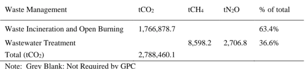
3.2.4 Waste Management

According to the GPC framework, the Waste Management sector contains four categories: Waste Landfill, Waste Combustion, Domestic Water Treatment and Industrial Water Treatment. However, due to the insufficient Solid Waste landfill data of Food Landfill, Clothing Landfill and Paper Landfill, only Waste Incineration and Open Burning and Wastewater Treatment are able to be accounted for, as shown in Table 8.

Table 8. Overview of GPC requested contents

Waste Management tCO2 tCH4 tN2O % of total

Waste Incineration and Open Burning 1,766,878.7 63.4%

Wastewater Treatment 8,598.2 2,706.8 36.6%

Total (tCO2) 2,788,460.1

Note: Grey Blank: Not Required by GPC

The first item is Waste Incineration and Open Burning, accounting for both Domestic Waste and Hazardous Waste. Data are collected from the

<City Sanitation Statistics> and the Beijing Municipal Environmental Bureau Official Website. It follows the equation below and outcomes are shown in Table 9.

Item Cement Production (t) Factor (tCO2/t production) Emission (tCO2)

Cement 568.4 0.54 3,058,127.0

Item Weight of Clinker Factor (tCO2/t clinker） Emission (tCO2)

Iron and Steel 256.4 1.8 4,692,120.0

CO2 Emissions＝∑Amount of Waste Combustion i× Rate of Carbon Content in Waste× i Rate of Mineral Carbon Content in Carbon Content i× Oxidation of Coal during combusting i×CO2- C Rate（44/12）

i Stands for different waste category from Domestic Waste or Hazardous Waste Table 9. Beijing 2012 GHG emission of Waste Incineration and Open Burning Category Amount of

combustion (t)

Factor (tCO2/t）

Carbon Content in Waste

Mineral Carbon Content

Oxidation of Coal

CO2- C

Emission (tCO2)

Domestic Waste

6,483,100.0 0.3 0.2 0.4 95% 3.7 475,594.0

Hazardous Waste

122,000.0 0.0 0.0 0.9 97% 3.7 117.0

Total (tCO2)

75,711.0

Note: 2011 data was applied for combustion of Hazardous Waste as it was the most recently available data.

Second, CH

emissions of Domestic Water and Industrial Waste Water are shown in Table 10 and Table 11 respectively. Meanwhile, NO

emissions of Domestic Wastewater and Industrial Wastewater Treatment are shown in Table 12. In this part, the 2011 emissions were accounted for since the latest data available were from the 2011 edition of the China Statistical Yearbook.

Table 10. Beijing 2011 GHG emission of Domestic Water Treatment

COD (t) Transition

BOD/COD

kgCH4/kg BOD tCO2

87,100.0 0.5 0.1 3,880.0

Table 11. Beijing 2011 GHG emission of Industrial Waste Water Treatment (CH4 Emissions) COD amount of Degradable

Organic Matter in Industrial Waste Water (t)

BOD/COD Transition

kgCH4/kg BOD tCH4

37,491,000.0 0.5 0.04 696.0

Table 12. Beijing 2011 GHG emission of Domestic Wastewater and Industrial Waste Water Treatment (N2O)

3.2.5 Agricultural Activity

Beijing’s Agricultural Activity Emissions incurs CH

and N

O emissions from three sectors, which are fertilization of crops, enteric fermentation from livestock and livestock manure management. The overview is shown in Table 13. Detailed outcomes of each sector’s discharge amounts are provided in Table 14, Table 15 and Table 16. Regarding emissions from livestock, there is a slight difference between enteric fermentation and manure management. This is due to the fact that hens are not ruminant livestock and therefore chicken manure is accounted for in the manure management factor, but not the enteric fermentation factor as per the requirements of the GPC (2014).

Nitrogen Content (N kg)

Factor

（kgN2O/kgN）

N2O-N Transition

（44/28）

tN2O

167,506,092 0.005 1.6 1,315

Table 13. Overview of Beijing 2012 Emissions of AFOLU

Category tCO2 tCH4 tN2O tCO2 % of Total

Fertilization of Crops 195.6 58,288.8 0.04%

Enteric Fermentation from Livestock

365,349.

2

409,130.

5 131,054,619.0 98.5%

Livestock Manure

Management 15,565.5 5,168.4 1,929,320.7 1.5%

Total tCO2 133,042,228.5

Note: Grey Blank: Not Required by GPC Table 14. Beijing 2012 Fertilization Emissions

Category Sown

Areas(ha)

Total Yield (t)

Emission Factor (t N2O/ha)

Emission Factor (t N/t)

Emission

(t N2O) % of total

Vegetables 64,090.4 0.002 134.6 68.8%

Tubers 2,132.6 0.001 2.6 1.3%

Wheat 52,183.0 0.001 52.2 26.7%

Soybeans 4,716.3 0.0003 1.4 0.7%

Tobacco Leaves 3.7 0.002 0.0 0.0%

Peanuts 12,400.4 0.0004 4.8 2.5%

Total (tCO2) 58,287.6

Note: Grey Blank: Not Required by GPC

Table 15. Overview of Beijing 2012 Emissions of Livestock Enteric Fermentation Category

Kg CH4/num ber/year

Number Emission(t CH4)

kg/number/y ear

Emissio ns (t N2O)

% of total Cattle and

Buffalo 80.1 1,873,900.0 150,146.2 46.7 87,448.7 22.7%

Sheep 8.1 25,963,500.

0 211,169.8 12.0 311,562.

0 74.9%

Goat 8.3 414,300.0 3,452.5 2.0 828.6 0.3%

Pig 1.0 580,700.0 580.7 16.0 9,291.2 2.1%

Subtotal 365,349.2 409,130.5

Total (t CO2) 131,054,610.0

Table 16. Overview of Beijing 2012 Emissions of Livestock Manure Management Category Number Factor:

KgCH4/Num ber/Year

Emissio n (tCH4)

Factor: Kg N2O/Number /Year

Emissio n tN2O)

% of total Cattle and

Buffalo

1,873,900 5.1 9,631.8 1.3 2,473.5 50.7

Sheep 25,963,500.0 0.2 3,894.5 0.1 2,414.6 42.3

Goat 414,300.0 0.2 70.4 0.1 38.5 0.7

Pig 580,700.0 3.1 1,811.8 0.2 131.8 4.4

Hens 15,696,000.0 0.0 157.0 0.0 109.9 1.9

Total (t CO2) 1,929,314.2

3.2.6 Forestry Activity and Other Land Use Change

Regarding Forestry and other Land Use Change sectors, emissions from forestry emissions, carbon sinks, combustion caused by land use and decomposition are requested. However, due to data limitations, only forestry emissions are calculable.

The final outcome of this forestry activity is a combination of emissions and carbon sinks. Among them, carbon sinks are negative numbers since they contribute to the absorption of emissions. Thus the total amount was - 0.01362tCO

. The method is divided into two, as shown in the following calculation:

Carbon Sink (tCO2

）＝

（

）

Carbon Emission

（

）＝

living wood × Average Density of wood × Biomass Conversion × Carbon Content × CO2- C Conversation

（

）

Table 17. Overview of Beijing 2012 Forestry Activity Algorithm

4. DISCUSSION AND CONCLUSIONS

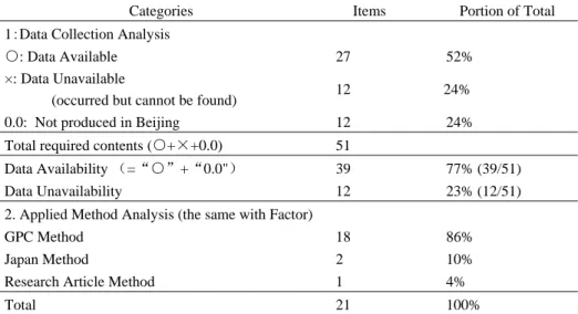
4.1 Data Availability Analysis

Table 18. Data availability and Method application Analysis

This study shows that data availability of the Beijing GHG emissions inventory is 77%. Details are shown in Table 18. Regarding the method, the

Stock M3

Growth Rate

Consumption Rate

Average Density t/m3

Biomass Conversion (All)

Biomass Conversion (Above Land)

Carbon Content

CO2- C Rate

Carbon Sink tCO2

Carbon Emission tCO2

29.2 6.4% 4.3% 0.5 1.8 1.4 0.5 44/12 -0.04 0.03

Categories Items Portion of Total

1：Data Collection Analysis

○: Data Available 27 52%

×: Data Unavailable

(occurred but cannot be found) 12 24%

0.0: Not produced in Beijing 12 24%

Total required contents (○+×+0.0) 51

Data Availability （=“○”+“0.0"） 39 77% (39/51)

Data Unavailability 12 23% (12/51)

2. Applied Method Analysis (the same with Factor)

GPC Method 18 86%

Japan Method 2 10%

Research Article Method 1 4%

Total 21 100%

usage rate of the GPC method is 86%. Meanwhile, other methods that include those from Japan and China account for 10% and 4% respectively.

4.2 Data Unavailability Analysis

In this paper, based on the GPC framework, 23% of the required items cannot be calculated due to data unavailability. However, these items account for a small portion. As shown in Table 3, those contents denoted with a “ × ”are not calculated items. However, most of them are not calculated by others, as in the case of Oita Prefecture. Based on the authors’

previous study, it can be found that the only item which was calculated by Oita, but not by this study, was Waste Landfill, which was 47,166 tCO

e and accounted for 0.11% of Oita’s total emissions (42,445,556 tCO

e).

4.3 Comparison Study between Beijing 2012 Emissions and Other Metropolitan Areas

This study compares Beijing’s 2012 emissions with six mega cities that include Shanghai (China), Tokyo (Japan), London (United Kingdom), Washington D.C. (United States), New York (United States) and Paris (France) with conclusions shown in Table 19.

Table 19. GHG Emission per capita and per GDP Comparison at a Global Level

First, from the GHG (tCO

) per capita perspective, Beijing’s 2012 emissions were the highest with 18.5 tCO

e. Specifically, it had a relatively large GHG emission gap between New York (6.5 tCO

) and Tokyo (4.91 tCO

). On the contrary, it was close to that of Shanghai, London and Washington D.C., with differences of 5.3 tCO

, 4.35 tCO

, and 4.21 tCO

respectively. Second, from the GHG emissions (tCO

) per GDP (104 RMB) perspective, Beijing’s emissions were the highest in 2012 as well. Third, regarding the reporting year, Table 19 presents that this study was the most up to date one in terms of disclosing city emissions. Fourth, regarding

Category Beijing (This study)

Shanghai (Zhao, Q., 2011)

Tokyo (Tokyo Metropolitan Government, 2014)

London (Greater London Authority (GLA), 2014)

Washington, D.C.

(District of Columbia, 2012)

New York (City of New York, 2012)

Paris (COP Cities 2012 Global Report, 2012)

GHG (tCO2)

per Capita 18.5 13.2 4.9 14.2 14.3 6.5 10.9

Gap: (Beijing 2012 vs. other cities)

-- 5.3 13.6 4.4 4.2 12.0 7.6

GHG(tCO2)/104

RMB GDP 2.4 1.3 0.1 0.5 0.4 0.1 0.1

Gap:(Beijing

2012 vs. others) -- 1.0 2.2 1.9 1.9 2.3 2.3

GDP

(10⁴ RMB) 160,004,000 136,981,500 481,340,440 243,882,013 220,717,280 829,174,580 382,050,240

Latest Data 2012 2008 2011 2010 2010 2010 2010

Primary Data Research Research Government PAS 2009 State

Government Government COP cities 2012 Report

availability of GHG emission reports, emissions from Japan, UK, the US and France were disclosed, while those from China were kept private.

Information on Tokyo, London, Washington D.C, New York and Paris were published through governments, international organizations’ reports and academic studies, while those of Beijing were not. GHG emissions from Chinese cities like Beijing can only be accessed through academic research.

4.4 Issues and Recommendations

In this study, four issues have been found and relative recommendations are provided and aggregated in Table 20. The first issue regards the consistency between the GPC’s activity data collection method and the Beijing Bureau of Statistics (BSY)’s activity data reporting method. Because the statistical methods are inconsistent, some emissions are not able to be accounted for. Hence, this study recommends that the GPC and BSY unify the data category.

The second issue is a boundary issue because boundary principles are ambiguous and boundary data is insufficient. Therefore, this study recommends that inventory authorities set and clarify boundary principles.

Furthermore, enriching boundary activity data is suggested to BSY.

The third issue is insufficient activity data. The evidence for this is shown in Table 20 and the main reason is that data provided by the Beijing Bureau of Statistics is insufficient. Therefore, this study recommends that the Beijing Bureau of Statistics enrich its data category.

The fourth issue is that there is no publicised emissions report from private enterprises, which makes accounting difficult. Hence, this study suggests that governments establish a private enterprise reporting scheme and make companies set mitigation goals.

Table 20.General Issues of Beijing’s 2012 Inventory and Recommendations

Issues Examples Recommendations Targets

Inconsistent inventory method and statistical category of activity data

1)Stationary Energy-Fossil Fuel CH4

2) IPPU Sector

Unify the data category GPC; BSY

Boundary issue on boundary at national level and domestic level

1)Stationary Energy- Scope 3 in balance sheet 2)Waste

Management Sector

1) Clarifying

boundary principles 2)Enrich boundary activity

data published by the urban Bureau of Statistics

International and Domestic inventory

setting authorities 2) BSY Lacking activity

data

1)Stationary:

Energy-Fugitive Emission and Biomass Fuel Combustion 2)Waste Management Sector: Landfill and combustion

Enrich categories of data (e.g., Biomass Fuel Combustion, Waste Combustion, Forest Combustion)

Beijing Bureau of Statistics

No public report from enterprises

Substitutes for Ozone Depleting Substances Sector

Establishing enterprise GHG emission reporting scheme

For government and enterprises

In conclusion, this study makes a preliminary Chinese city inventory by accounting Beijing city’s GHG emissions. Through combining the GPC method, the Japanese method and the method reached in a previous research article, it creates a timely and relatively complete GHG emission inventory.

Furthermore, this study enables global comparisons between Beijing and other mega-cities. Additionally, this research also identifies issues and provides four recommendations to improve GHG inventory accounting in Beijing.

ACKNOWLEDGEMENTS

This work was supported by grants from the Japan Society for the Promotion of Science (KAKENHI No. 26420634).

REFERENCES

Bai, W., Zhuang, G., Zhu, S., & Liu, D. (2013). "Discussion of Four Issues About Inventorying Urban Greenhouse Gas Emissions in China". Progressus Inquisitiones DE Mutatione Climatis, 9(5), 335-340.

Beijing Municipal Environmental Monitoring Center. (1994). "Beijing Greenhouse Gases Emission and Abatement Research".

Cai, B. (2012). "Research on Greenhouse Gas Emissions Inventory in the Cities of China".

China Population,Resources and Environment, 22(1), 21-27.

China Statistics Press. (2012). Beijing Statistical Yearbook 2012. Beijing: China Statistics Press.

City of New York. (2012). "Inventory of New York City Greenhouse Gas Emissions, December 2012". Retrieved from http://s-

media.nyc.gov/agencies/planyc2030/pdf/greenhousegas_2012.pdf on Nov, 2015.

CNN Beijing. (2014). "U.S. And China Reach Historic Climate Change Deal, Vow to Cut Emissions". Retrieved from http://edition.cnn.com/2014/11/12/world/us-china-climate- change-agreement/ on May, 2015.

COP Cities 2012 Global Report. (2012). "Per Capita Ghg Emissions for C40 Cities".

Retrieved from http://smedia.nyc.gov/agencies/planyc2030/pdf/greenhousegas_2012.pdf on Nov, 2015.

Deng, N., Chen, G., Cui, W., Zhang, Y., & Ma, H. (2013). "Municipal Greenhouse Gases Inventory and Analysis: A Case of Tianjin". Journal of Tianjin University Science and Technology, 46(7), 635-640.

Dhakal, S. (2004). "Urban Energy Use and Greenhouse Gas Emissions in Asian Mega- Cities". Institute for Global Environmental Strategies, Kitakyushu, Japan.

District of Columbia. (2012). "Reducing Greenhouse Gas Emissions While Growing the City". Retrieved from

http://doee.dc.gov/sites/default/files/dc/sites/ddoe/publication/attachments/GHGinventory- 1205-.pdf on Nov, 2015.

Environmental Affairs Office of Oita Prefecture. (2015). "Ghg Inventory for Oita Prefecture".

Retrieved from http://www.pref.oita.jp/10400/advice/bosyu/h17/ondanka/data/shiryou.pdf on May, 2015.

GPC. (2014). "Global Protocol for Community-Scale Greenhouse Gas Emission Inventories (Gpc): An Accounting and Reporting Standard for Cities". Retrieved from http://ghgprotocol.org/files/ghgp/GHGP_GPC.pdf

Greater London Authority (GLA). (2014). "Application of Pas 2070 - London, United Kingdom, an Assessment of Greenhouse Gas Emissions of a City". Retrieved from http://shop.bsigroup.com/upload/PAS2070_case_study_bookmarked.pdf on Nov, 2015.

Guo, S., Shao, L., Chen, H., Li, Z., Liu, J. B., Xu, F. X., . . . Chen, Z. M. (2012). "Inventory and Input–Output Analysis of Co² Emissions by Fossil Fuel Consumption in Beijing 2007". Ecological Informatics, 12, 93-100.

Intergovernmental Panel on Climate Change (IPCC). (2006). "2006 Ipcc Guidelines for National Greenhouse Gas Inventories, Prepared by the National Greenhouse Gas

Inventories Programme, Eggleston H.S., Buendia L., Miwa K., Ngara T. And Tanabe K.

(Eds). ". Retrieved from www.ipcc-nggip.iges.or.jp/public/2006gl

International Council for Local Environmental Initiatives (ICLEI). (2013). "U.S. Community Protocol for Accounting and Reporting of Greenhouse Gas Emissions". Retrieved from http://icleiusa.org/publications/us-community-protocol/ on July, 2015.

International Energy Agency (IEA). (2009). "Co² Emissions from Fuel Combustion 2009- Highlights". Retrieved from http://www.iea.org/co2highlights/co2highlights.pdf on May, 2015.

Japanese Ministry of Environment. (2010). "Manual of Planning against Global Warming for Local Governments". Retrieved from

http://www.env.go.jp/earth/ondanka/sakutei_manual/manual_kani1008/full.pdf on July, 2015.

Sovacool, B. K., & Brown, M. A. (2010). "Twelve Metropolitan Carbon Footprints: A Preliminary Comparative Global Assessment". Energy Policy, 38(9), 4856-4869.

Tokyo Metropolitan Government. (2014). "Tokyo 2011 Emissions". Retrieved from http://www.kankyo.metro.tokyo.jp/climate/other/emissions_tokyo.html on Nov, 2015.

Wang, P. (2013). "Estimation of Greenhouse Gas Emissions for Nantong". Environmental Monitoring in China, 29(4), 147-151.

Yuan, X. H., & Gu, C. L. (2011). "Urban Greenhouse Gas Inventory and Methods in Beijing". Urban Environment & Urban Ecology, 24(1), 5-8.

Zhang, L., Hu, Q., & Zhang, F. (2014). "Input-Output Modeling for Urban Energy Consumption in Beijing: Dynamics and Comparison". PLoS ONE, 9(3), e89850.

Zhang, M., Suo, A., Wang, T., & Ge, J. (2012). "Estimation on Beijing Co² Emissions".

Paper presented at the 8th Biennial Conference of Chinese Ecological Economics Society, Urumchi, Xinjiang.

Zhao, Q. (2011). "Shanghai Ghg Inventory Study". (Master), Fudan University.

Zhao, R., Huang, X., Zhong, T., Liu, Y., & Chuai, X. (2014). "Carbon Flow of Urban System and Its Policy Implications: The Case of Nanjing". Renewable and Sustainable Energy Reviews, 33(2), 589-601.

Zhao, Y. Q., Li, X. C., & Li, G. J. (2012). "Current Situation of Co² Emission and Point Sources Distribution in China's Iron and Steel Industry". Journal of Iron and Steel Research, 24(5), 1-4.

Zhu, S. (2009). "Present Situation of Greenhouse Gas Emission in Beijing and the Approach to Its Reduction". China Soft Science, 9, 93-106.