Measuring Deformed Sea Ice Area in Seasonal Ice Zones Using L-band SAR Images
Takenobu Toyota1, Junno Ishiyama2 and Noriaki Kimura3
1Institute of Low Temperature Science, Hokkaido University
2Toma Town Office, Hokkaido
3Atmosphere and Ocean Research Institute, University of Tokyo
Introduction
For better performance of the numerical sea ice models for the Arctic Ocean, the need to improve the dynamic part in the model has been pointed out. Since the fraction of the seasonal ice zone (SIZ) in the Arctic Ocean is increasing, it will become more and more important in the future to understand the dynamical processes of sea ice in the SIZ. Therefore, developing the measures to detect deformed ice area from satellite images is expected to contribute significantly to the improvement of numerical sea ice models. To monitor the deformed ice area, the space-borne Synthetic Aperture Radar (SAR) is a useful tool because of its high spatial resolution (≤100 m), wide coverage (≥100 km), and high sensitivity to surface roughness. While C-band SAR has been used most frequently for the polar sea ice research, L-band SAR was shown to be more suitable for discriminating ridged ice from level ice than C-band SAR (e.g., Dierking and Busch, 2006). However, to the authors’ knowledge, measures for classification into ridged ice with L-band SAR has not been developed. The purposes of this study are to develop measures to extract deformed ice area in SIZ using PALSAR imagery at a ScanSAR mode, based on field experiments, and to examine the factors which can affect the availability of L-band SAR for detecting deformed ice area quantitatively.
Data
In the analysis, we used three satellite SAR sensors (PALSAR, RADARSAT-2, PALSAR-2), all of which were observed at a ScanSAR mode to cover a wide area of the southern Sea of Okhotsk. PALSAR images were used to develop measures to classify sea ice types, based on the field experiments aboard the PV “Soya” during 2009-2011. To compare the ability of detecting deformed ice between L-band and C-band SARs, one RADARSAT-2 image, which was selected so that the observation time was the closest to one of PALSAR images, was analyzed with the PALSAR image. PALSAR-2 images were used to validate the measures developed with PALSAR imagery, and to examine the availability of backscatter coefficients at HV polarization (σHV0), compared with σHH0, based on the field experiments for four years (2016-2019).
Among the data obtained during the field experiments, photos taken hourly from the upper deck of the ship, aero-photos taken from the helicopter, ice thickness data measured by means of a shipborne video system, and hourly visual observations according to the Antarctic Sea Ice Processes & Climate (ASPeCt) protocol (http://aspect. antarctica.gov.au/) were mainly used for analysis. Based on the photos, sea ice was categorized into three ice types: nilas (thin level ice), pancake (thin rough ice), and deformed ice (thick rough ice). Besides, the datasets of the ice drift and meteorological reanalysis are also used as supplementary data for analysis.
Analytical methods and results
Development of measures with PALSAR image
Considering that the penetration depth of L-band radar is about 0.3 - 0.5 m for first-year ice and the radar signal is sensitive to the surface roughness at a scale greater than its wavelength (0.24 m), σHH0 of L-band SAR is expected to discriminate deformed ice from pancake ice and nilas. Since σHH0 depends significantly on θi, we attempt to develop measures to classify sea ice into these three categories as a function of σHH0 and θi. Based on 24 samples, the following threshold lines were derived: (1) σHH_pd0
= -0.197θi -7.55 (dB) between deformed ice and pancake ice, and (2) σHH_np0= -0.194θi -11.51 (dB) between pancake ice and nilas. The upward deviation from (1), referred to as HH anomaly, is expected to be an indicator of the degree of deformation.
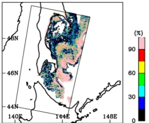
With this threshold line, the features of temporal evolution of deformed ice area were examined by mapping from January to March in 2010. In these figures, it is found that deformed ice area is characterized by large temporal variability and rather aligned distribution with about a few tens of km in width and about a few hundreds of km in length. One example of deformed ice area on Feb. 22, 2010, is shown in Fig.1. In the comparative analysis between PALSAR and RADARSAT-2, we focused on how the RADARSAT-2 image represents the ice types judged from PALSAR-derived measures, as expressed by (1) and (2), for the cross-section line and two characteristic areas. The result indicates that L-band SAR is much more useful to discriminate deformed ice from thin level ice or thin rough ice, compared with C-band SAR, which is consistent with past studies (e.g., Dierking and Busch, 2006).
Further examination with ALOS-2/PALSAR-2 images
Our measures are tested for PALSAR-2, which has the additional functions of dual polarization at ScanSAR mode and a wider range of θi, to examine their effectiveness and the properties of dual polarizations. Since the ice conditions for four year (2016- 2019) were significantly different, it serves to understand which factors can affect our measures for detecting deformed ice. Ice thickness measurements and ASPeCt observations show that newly formed ice covered a wide area in this region in 2016 (pancake ice) and 2019 (nilas), whereas developed ice was prominent in 2017 and especially 2018. Another significantly different feature is dominant floe size: pancake ice in 2016, 2-20 m in 2017, 20-100 m in 2018, and nilas in 2019.
From validation with photos, it is shown that our measures represent the real conditions well. On the other hand, it is also revealed from the comparative analysis between four years along the same cross section line that the order of four years for HH anomaly (2019<2016≈2018<2017) does not coincide with that for degree of deformed ice observed. As for σHV0, the degree of deformed ice is measured by the deviation from σHV_ow0 = -0.636 θi -5.78 (dB), which shows the dependence of σHV0 at ocean (flat) surface on θi, referred to as HV anomaly. Although σHV0 was shown to be sensitive to surface roughness, again it is revealed from cross section analysis that the order of four years for HV anomaly (2019<2016<2018<2017) does not coincide with that for degree of deformed ice observed. Considering that for a given ice area the total length of the boundaries between sea ice and seawater becomes longer as the floe size becomes smaller, we infer that the radar backscatter is affected by floe size distribution through reflection at the ice margin, as shown in Fig. 2. This may explain relatively higher radar signals along the marginal ice zone in Fig. 1 and also cautions us to take the floe size conditions into account as well as ice deformation when applying our measures. Our rough estimate indicates that 4 times the total perimeter (i.e., 1/4 floe size for the same sea ice area) is comparable to about twice the ice surface roughness and enhance σHH0 at L-band by 4-6 dB.
Conclusions
For better understanding of deformation processes in the seasonal ice zone, we developed measures to detect deformed ice area using ALOS/PALSAR images as a preliminary step. Our results show that 1) forced by winds and ocean waves, deformed ice area is quite variable with both time and space. In the inner ice pack region, the temporal evolution of deformed ice area was consistent with the convergence/divergence zone of ice drift, 2) both σHH0 and σHV0 are affected significantly not only by ice surface roughness but also by floe size distribution through the total perimeter of sea ice floes, and 3) the relative contribution of floe size distribution to the radar signals is estimated to be larger at HV polarization than at HH polarization by a few dB.
Acknowledgments
Observations in the Sea of Okhotsk were conducted in collaboration with Japan Coast Guard, PV “Soya”. ALOS/PALSAR and ALOS-2/ PALSAR-2 images were provided by JAXA through the ALOS Research Project (PI: No.573) and the 2nd Research Project on the Earth Observations (PI: ER2A4N012).
References
Dierking, W. and T. Busch, Sea ice monitoring by L-band SAR: An assessment based on literature and comparisons of JERS-1 and ERS-1 imagery, IEEE Trans. Geosci. Remote Sens., 44(2), 957-970, 2006.
(a)
(b)
Figure 2. Schematic pictures, showing how floe size distribution affects the radar signals for (a) 2016 and (b) 2018.
In the figures, red and blue arrows denote backscattering at the deformed ice surface and ice margins, respectively.
Figure 1. One examples of deformed ice area fraction, determined by (1), on Feb 22, 2010.