Digital Halftoning : Formulation as a Combinatorial Optimization Problem and Approximation Algorithms Based on Network Flow (Algorithm Engineering as a New Paradigm)

Digital Halftoning: Formulation

as a

Combinatorial

Optimization Problem and Approximation Algorithms

Based

on

Network Flow

Tetsuo

Asano1

, Naoki

Fujikawa1

, Naoki

Katoh2,

Tomomi

Matsui3,

Hiroshi

$\mathrm{N}\mathrm{a}\mathrm{g}\mathrm{a}\mathrm{m}\mathrm{o}\mathrm{C}\mathrm{h}\mathrm{i}4$,

Takeshi

Tokuyama5,

and Nobuaki

Usui6

1School

of Information Science, 2 _{Graduate School of Engineering,}

JAIST Kyoto University

Tatsunokuchi 923-1292, Japan Kyoto 606-8501, Japan

$\mathrm{t}[email protected] [email protected]

3 _{Graduate School of Engineering,} 4 _{Dept. of Information and Computer Sciences,}

University ofTokyo Toyohashi University of Technology

Tokyo 113-8656, Japan Toyohashi 441-8580, Japan

tomomi@misojiro.$\mathrm{t}$.u-tokyo.ac.jp naga@ics.$\mathrm{t}\mathrm{u}\mathrm{t}$.ac.jp

5 _{Graduate School of Information Sciences,} 6 _{Peripheral Systems Laboratories,}

Tohoku University Fujitsu Laboratories Ltd.

Sendai 989-3201, Japan Atsugi 243-0197, Japan

[email protected].$\mathrm{a}\mathrm{c}$

.

jp [email protected] itsu.co.jp

Abstract: Digitalhalftoning is an important technique to convert animage having several

bits for brightness levels into a binary image consisting of black and white dots which looks

similarto aninput image. Thesimilaritybetween twoimages is measuredbythe totalsumof

differences inthe weighted sumsof brightness levelsofpixelsin a neighborhood surrounding

each pixel. Then, the problem of producing an optimal halftoned image is a combinatorial

optimization problem to find a binary image minimizing the measure for a given

multiple-level image. Despiteanegative result that it is $\mathrm{N}\mathrm{P}$-completeevenfor asimple neighborhood

consisting of$2\cross 2$ pixels, we can rely onapproximation algorithms mainlybased on network

flow algorithms.

Keywords: approximation algorithm, combinatorial optimization, discrepancy, matrix

rounding, network flow

1

Introduction

The quality of color printers has been drastically

improved in recent years, mainly based on the

development of fine control mechanism. On the

other hand, there seems to be no great

inven-tion on the software side of the printing

tech-nology. What is required is a technique to

con-vert an intensity image having several bits for

brightness levels into a binary image consisting

of black and white dots so that the binary image

looks very similar to the input image. Theoret-ically speaking, the problem is how to

approx-imate an input gray image by a binary image.

Sincethis is oneof the centraltechniques in

com-putervision and computer graphics, a great

num-ber of algorithms have been proposed (see, e.g.,

[12, 10, 6, 13, 14]$)$. However, there have been

very few studies discussing reasonable criteria for

evaluating the quality of output binary images;

maybe because the problem itselfis very

practi-cally oriented. Actually, the most popular

crite-rion is tojudge the quality by human eyes. It is

desirabletoestablishagood evaluation system of

halftoning methods (instead of the “humaneye’s

judgment”), and to handle the digital halftoning

problem fully mathematically. Unfortunately, to

the authors’ knowledgenomathematicalcriterion

has not been a main focus on digital halftoning

even

in the comprehensive studies in the Ph.D.

So, one of the purposes of this paper is to

set-tle some reasonable mathematical criterion for

this problem based on a model for human visual

perception. Although there are extensive studies

on human visual perception (see, e.g., [16]), we

use a simplified model to analyze computational

complexity of the problem. Our criterion

mea-sures the ”difference” between the average gray

levels

or

the total sums of levels normalized

be-tween $0$ and 1 in a neighborhood surrounding

each pixel. Then, the problem of producing an

optimal halftoned image is a combinatorial

opti-mizationproblemtofindabinaryimage

minimiz-ing the measure for agiven multiple-level image.

The complexity of the problem depends on the

choice ofthe neighborhood family. In most cases

it is $\mathrm{N}\mathrm{P}$-hard. Actually, we show that it is the

case even if each neighborhood consists of $2\cross 2$

pixels.

Although the problem itself is defined in the

two-dimensional plane, it is possible to define its

one-dimensional version in which a sequence of

real numbers is given. This problem itself is an

interesting combinatorial problem, $\dot{\mathrm{a}}$

nd we show

that it canbe solvedin polynomialtime byusing

negative cycle detection algorithms.

This implies that it is essentially necessary

to consider approximation $\mathrm{a}\mathrm{n}\mathrm{d}/\mathrm{o}\mathrm{r}$heuristic

algo-rithms. $\mathrm{E}\mathrm{v}\mathrm{e}\mathrm{n}.\mathrm{f}_{\mathrm{o}\mathrm{r}}$ the $\mathrm{t}_{\mathrm{W}\mathrm{O}-}\mathrm{d}\mathrm{i}\mathrm{m}\mathrm{e}.\mathrm{n}$sional problem,

if each neighborhood is one-dimensional along a

space-filling curve, we can apply the algorithms

for the one-dimensional case. The use of

space-fillingcurves is popular in image processing, and

we think this method (although it is merely a

heuristic method since neighborhood should be

truly $\mathrm{t}\mathrm{w}\mathrm{o}^{-}\mathrm{d}\mathrm{i}\mathrm{m}\mathrm{e}\mathrm{n}\mathrm{s}\mathrm{i}_{0}\mathrm{n}\mathrm{a}\mathrm{l}$in practice) is probably

useful if we can generate space-filling curves in

somewhat random$\mathrm{m}\mathrm{a}\mathrm{n}\mathrm{n}\mathrm{e}\mathrm{r}[4]$

.

We evaluate some

popular error-propagating algorithms in digital

halftoning in our optimization criterion.

2

Known

Basic

Algorithms

Given an$N\cross N$array$A$of real numbers between

$0$ and 1, we wish to construct a binary array $B$

of the same size which looks similar to $A$, where

entry values represent light intensities at

corre-sponding locations. The most naive method for

obtaining$B$is simply to binarize each input value

by a fixed threshold, say 0.5. It is simplest, but

the quality of the output imageis worst since any

uniformgray region becomes totally white or

to-tally black. The most important is how to

repre-sent intermediateintensities. Amonganumberof

algorithms for digital halftoning well-known are

Ordered Dither and Error Diffusion. We briefly describe them.

2.1

Ordered Dither

Instead of using a fixed threshold over an

en-tire image, this method uses different

thresh-olds. A simple way of implementing this idea

is as follows: We prepare a square submatrix

of $M\cross M$ entries which are integers ranging

from $0$ and $M^{2}-1$ and tile an input array by

this submatrix. Then, for each entry $(\dot{i},j)$ we

have an input value $A(\dot{i},j)$ in $A$ and an

inte-ger $D(i\mathrm{m}\mathrm{o}\mathrm{d}M,j\mathrm{m}\mathrm{o}\mathrm{d}M)$ in the submatrix. If

$A(\dot{i},j)$ $>D$($i\mathrm{m}\mathrm{o}\mathrm{d}M,j$ mod $M$)$/M^{2}$ then the

corresponding output value$B(i,j)$ is determined

to be 1, and otherwise it is $0$

.

This submatrix

is called a dither matrix. An example is shown

$\mathrm{b}\mathrm{e}\mathrm{l}\mathrm{o}\mathrm{w}[12]$.

2.2 Error Diffusion

Ordered Dither is simple and efficient, but its

output quality is not satisfactory in many cases.

Another standard method uses a fixed

thresh-old 0.5 but it diffuses the quantization error

over unprocessed neighboring pixels according

to some fixed ratios. The ratios suggested by

Floyd and Steinberg in their paper [10] are

(7/16, 3/16, 5/16, 1/16) for the right, lower left,

lower, and the lower right pixels, respectively.

This method gives excellent results inmany cases,

but it tends to generate some visible patterns in

an areaof uniform intensity, whichare caused by

2.3

Related Combinatorial Problems

The quality of the ordered dither method

heav-ily depends

on

the dither matrix. The matrix

shown above is constructed according to asimple

rule, which is known as Incremental Voronoi

In-sertion. That is, westart withanarbitrary entry.

Sincethesubmatrix tiles the entire plane, wehave

many copies of the entry. Then, we choose the

entry farthest from the existing points (entries).

Such a point must be avertex of the Voronoi

di-agram. Thus, ourstrategy is to choose aVoronoi

vertex that is farthest from the existing points. This selection is iterated until half of the entries

are chosen. The remaining half is filled in

sym-metrically.

Now we have a natural question. Does this

strategy optimize anything? Imagine a part of

an image in which intensities gradually increase.

Then, the number (or density) of white dots also

increases according to the dither matrix starting

from a dark part consisting of only O-numbered

entries until an entirely bright part. During the

transition, white dots should be uniformly

dis-tributed. This means that for any $k,$ $0\leq k\leq$

$M^{2}/2$ those entries having numbers greater than

orequalto $k$ must be asuniformly distributedas

possible. The uniformitycanbe measured by the

ratio of the minimum pairwise distance over the

diameter ofthemaximum empty circle. A

combi-natorial problem related to this is to find apoint

sequence that minimizes the maximum of the

ra-tios defined above. It is rather easy to see that

the incremental Voronoi insertion is not optimal,

but it is open to find such anoptimalsequence.

An easier combinatorial problem is to

dis-tribute a given number of points within a unit

square. This problem has been studiedfor many

years in combinatorics under the name of

Pack-ing Problem. Therewas abreak-through recently

in this study which shows best packing patterns

up to about 50 points and proved the optimality

of their packing patterns consisting of up to 26

points. In our case the base plane is not

contin-uous but discrete. If the size of the grid plane is

small enough, say, $16\cross 16$, we can find an

opti-mal solution by solving an integer programming

on 256 variables.

Another related problem

comes

from the

hu-man perception. An interesting feature of

hu-man perception is that horizontal and vertical

patterns are more sensitive to human eyes than

skewed patterns. This fact suggests

us

of

a

ro-tated dither matrix. Then, the problem is how

to design sucharotated pattern consisting of$M^{2}$

elements. This is not so easy. In fact, to the

authors’ best knowledge only one method [17] is

known. It is a rotation by a so-called rational

angle defined by triangles of edges with integral

lengths. We have developeda scheme for

achiev-ingrotation ofasquaredregion approximately by

any given angle. The detail will be described in the final report.

3

Why

Raster Scan

Error Diffusion is one of the most popular

meth-ods for digital halftoning. One of the drawbacks

of this method is that it tends to generate

reg-ular patternings, which are caused by fixed scan

order andfixed coefficients forerrordiffusion. For

better quality we need to incorporate some

ran-domness. Thus, we come up withan ideato use

randomspace-fillingcurvesinstead of rasterscan.

Recently, it has been observed that error

diffu-sion along somespace-fillingcurvessuchasPeano

curvesand Hilbertcurvessometimes achieve

bet-ter quality compared with the traditional error

diffusion basedon araster scan. One drawback of

the methodscomesfrom the fact that such

space-filling curves areusually defined recursively on a

square grid plane. Thus, there is some difficulty

when theyareapplied to rectangularimages.

An-other drawback is found in its quality ofan

out-put image due to its recursive structure. Since it

is recursively defined, each quarter of an image

is completely separated and their boundaries are

often visible in the resulting binary image.

The idea of using space-filling curves for

digi-tal halftoning is not new. Velho and Gomes [19]

use space-filling curves for cluster-dot dithering.

Zhang and Webber [20] give a parallelhalftoning

algorithm based on space-filling curves. Asano,

Ranjan, and Roos [5] formulate digital halftoning

as amathematical optimizationproblem and

ob-tainanapproximation algorithm basedon

space-filling curves. So, the digital halftoning

tech-niques based on space-filling curves seem to be

promising. However, one of their serious

size, that is, the size ofan input image must be

something like a power of 2 since most of

recur-sively defined space-filling curves are defined for

square lattice planes of sizes being such.

We have developed atheory for random

space-fillingcurves. One$\mathrm{r}\mathrm{e}\mathrm{s}\mathrm{u}\mathrm{l}\mathrm{t}[3]$isasimpleway of

gen-erating a random space-filling curves for a

rect-angular grid ofeven length in each side. It first

constructs a random spanning tree on a smaller

gridof the half side lengths and then generates a

tour along the tree. It runs in linear time in the

image size.

Another way of generating a random

space-filling curve without any size constraint is also

$\mathrm{p}\mathrm{r}\mathrm{o}\mathrm{p}\mathrm{o}\mathrm{S}\mathrm{e}\mathrm{d}[4]$. It is based on the following fact:

any space-filling curve is represented by regular

arrangement of stones in such a way that white

stone always lies to the right of the curve and

black stone does to the left. Then, a

space-fillingcurvewithout selfintersection corresponds

to an arrangement of stones in such a way that

no cross of different colors is included and there

are two connected components of those stones of

the samecolor, wheretwo stones areconnected if

they have the same color and they are adjacent

horizontallyorvertically. Then,asfaras a

condi-tion called parity condicondi-tion is satisfied, there is a

space-fillingcurvewithspecified starting and exit

entries. Moreover, defining an operation called

flipping which changes the curve locally by

ex-changing two stonecolors, we canguarantee that

for any two space-fillingcurves one canbe

trans-formed to another by successive flippings. This

suggests generation of random space-fillingcurves

by successive random flippings.

4

A

Mathematical Formulation

of

Digital Halftoning

Themain taskofthissection isto define the

dig-ital halftoning problem as a combinatorial

opti-mization problem by defining a reasonable

con-crete mathematical criterion. As we defined in

theintroduction, let $A=(a_{ij})_{i,jN}=1,\ldots,,$ $0\leq a_{ij}\leq$

$1$, be a matrix representing an image in the grid

array $G$ofsize $N\cross N$.

Imagine that we look at somepixel $(\dot{i},j)$ of the

gray-levelimage$A$

.

What happens is,weactually

perceivean average ofgray levelsofsome (small)

neighborhood of that point. Using the same

ob-servation, the intensity around the pixel $(\dot{i},j)$ of

a binary image is proportional to the number of

whitepoints in the corresponding neighborhood.

Therefore, density values should be roughly equal

around any pixel between an output binary

im-age of the digital halftoning and the input image

$A$

.

The observation motivates us to give the

fol-lowing mathematical formulation:

For anyregion$R$in the gridarray $G$ (regarded

as an $N\cross N$ rectangle subdivided into $N^{2}$

pix-els each of which corresponds to an array

en-try), we consider an error function $E^{R}(A, A’)$

describing the difference between two pictures

$A$ and $A’$ within the region $R$

.

A typical

er-ror function is the

_difference

_of

average density

$|A(R)-A’(R)|/|R|$, where $A(R)$ isthe sumof

en-tries of$A$ located in $R$, and $|R|$ is the number of

pixels in $|R|$

.

A family$\mathcal{F}$ofregions in_$G$ is calleda

neighbor-hood family if there exists a map $\phi$ from $G$ to $\mathcal{F}$

such that the region $\phi(p)\in \mathcal{F}$contains the pixel

$p$ for each pixel $p\in G$

.

We call $\phi(p)$ the

neigh-borhood of$p$

.

The map $\phi$ need not be surjective

nor injective. Note that this is a quite weaker

definition than the neighborhood system in usual

geometry. For a neighborhood family $F$, we

de-fine the $L_{\infty}$ distance

$Dist_{\infty}^{\mathcal{F}}(A, A’)= \max E^{R}R\in \mathcal{F}(A, A’)$

between the images $A$ and $A’$ with respect to

$\mathcal{F}$ and the error function $E$

.

This distance

is also called the maximum error between $A$

and $A’$ (with respect to $\mathcal{F}$). We only

con-sider the $L_{\infty}$ distance in this paper for

techni-cal reason, although the $L_{p}$ distance defined by

$( \sum_{R\in \mathcal{F}}(E^{R}(A, A’))p)^{1/}p$ might be a useful

mea-sure in practice.

Wemainlyconsider thefollowing family$\mathcal{F}$

con-sisting of (axis parallel) rectangular regions of a

fixed shape $l\cross k$. For an $l\cross k$ rectangular

re-gion $W$ in $G$, its center is the pixel _$p(W)$ on

the $\lceil l/2\rceil$-th row and $\lceil k/2\rceil$-th column counted

from the north-west corner of $W$

.

Note that

$p(W)$ has the center of gravity of$W$ in the

clo-sure of the pixel. We denote $W$ as $W(\dot{i},j)$ if

$p(W)=(\dot{i},j)$

.

This defines the neighborhoods

for the pixels (called central pixels) $(\dot{i},j)$

satisfy-ing $\lceil l/2\rceil\leq i\leq N-\lceil(l-1)/2\rceil$ and $\lceil k/2\rceil\leq$

(callednear-boundarypixels),wedefine its

neigh-borhood as the neighborhood of its nearest

cen-tral pixel with respect to the Euclidean metric.

This correspondence makes $\mathcal{F}$ to be a

neighbor-hood family

Consideran input images $A$ andits output

bi-nary image$B$ in the digital halftoning. If the

dif-ference between the average gray level near each

pixel image is small, the picture $B$ is expected

to look very similar to the original picture $A$; at

least $B$ is avery good approximation of$A$

(with-out further knowledge of the contents ofthe

im-age). Let us consider our neighborhood system.

The number $|W(\dot{i},j)|$ ofpixels inaneighborhood

is independent of the choice of $(\dot{i},j)$. With that,

instead of the difference ofaverage density, it is

natural to use

$E^{W(i,j)}(A, B)=|A(W(\dot{i},j))-B(W(\dot{i},j))|$

.

to evaluate the visual difference near $(\dot{i},j)$

be-tween $A$ and $B$, where $A(W(\dot{i},j))$ is the sum of

elements of$A$ within $W(\dot{i},j)$

.

Note-

_that.

we do not claim that our choice of

the

ne.ighborhood

family and the error function

is the best for evaluatingpracticaldigitalimages:

A broader $\mathrm{n}\mathrm{e}\mathrm{i}\mathrm{g}\mathrm{h}\mathrm{b}\mathrm{o}\mathrm{r}\overline{\mathrm{h}}\mathrm{o}\mathrm{o}\mathrm{d}$ family is probably

bet-ter, and the error function can be generalized in

various ways adapting to real applications, e.g.,

by assigning larger weights to the pixels nearer

to the center $(\dot{i},j)$ in the neighborhood to take

the summation; however, we consider the above

simple model to investigate the complexity of its

optimization. We discuss some broader choice of

the neighborhood family in Section 5.3.

Our goal . _{is to bring}

the local error $E^{W(i,j)}(A, B)$ _close to $0$ for any

pixel $(\dot{i},j)$; That is, to minimize the $L_{\infty}$ distance

$D_{\dot{i}}st^{\mathcal{F}}\infty(A, B)$

.

Hence, we have the following

for-mulation ofthe digital halftoningproblem:

Design a method to compute a binary

image $B$ such that $D_{\dot{i}}st^{\mathcal{F}}\infty(A, B)$ is as

smallas possiblefor an input image $A$

.

For simplicity, we write $D_{\dot{i}}st(A, B)$ for

$D\dot{i}st_{\infty}^{\mathcal{F}}(A, B)$ unless we want to emphasis the

neighborhood system $F$, error function, $\mathrm{a}\mathrm{n}\mathrm{d}/\mathrm{o}\mathrm{r}$

the $L_{\infty}$ measure. In particular, the binary

im-age $B$ minimizing $D_{\dot{i}}st(A, B)$ is called the

opti-mized digital approximation of$A$ (withrespect to

the neighborhood family $\mathcal{F}$). We investigate the

time complexity of computing the optimized

dig-ital approximation.

5

One dimensional

problem

If$l=1$, each member in $\mathcal{F}$ is a horizontal strip

of length $k$, and the problem can be solved on

each row independently. Therefore, we first

con-sider the one-dimensional version of theproblem.

Let $a=(a_{1}, a_{2}, \ldots, a_{n})$ be arational vector such

that $0\leq a_{j}\leq 1$ for all $j\in\{1,2, \ldots , n\}$ and $k$

be an integer with $1\leq k\leq n$

.

We consider the

neighborhood family$\mathcal{I}_{k}$ consisting of intervals of

length $k$

.

If$k$ is a constant, it is relatively easy

to design a linear time algorithm in $n$ by using

dynamic programming (in precise, $O(2^{k}n)$ time

using $O(2^{k}+n)$ _{space) to} compute the_optimized

digital approximation $b$. However, it is

nontriv-ial to design analgorithm which is polynomial in

both $n$ and $k$.

5.1 Polynomial

time

algorithms

The one-dimensional optimized digital

approx-imation of $a$ is the binary vector $b$ $=$

$(b_{1}, b_{2}, ’. . , b_{n})$ which is the solution of the

follow-ing integer programmfollow-ing problem, where $z$

cor-responds to the distance between $a$ and $b$ in our

measure:

minlmlze $z$

subject to $-Z \leq\sum_{j=}^{i+k}i(aj-bj)\leq z$ (1)

$(\forall\dot{i}\in\{1,2, \ldots, n-k\})$, (2)

$b_{j}\in\{0,1\}(\forall j\in\{1,2, \ldots, n\})$.

Since the variables $b_{1},$

$\ldots,$$b_{n}$ are 0-1 valued,

we can replace the inequality constraints (1) by

$\lfloor_{Z+}\sum_{j}^{i+}=i\rfloor ka_{j}\geq\sum_{j=}^{i+k}ib_{j}$

$\geq\max\{\lceil-Z+\sum^{i+k}j=ia_{j}\rceil, 0\}$

$(\forall\dot{i}\in\{1,2, \ldots, n-k\})$

.

We introduce the variables$x_{0},$ $\ldots,$$x_{n}$ satisfying

$x_{i}-x0=b_{1}+\cdots+b_{i}$ for $\dot{i}\in\{1,2, \ldots, n\}$

.

Then

the aboveproblemis transformed to the following

problem

minlmlze $z$

subject to

$x_{i+k}-x_{i-1} \leq\lfloor_{Z+}\sum_{jj}^{i+k}=i\rfloor a$

$(\forall\dot{i}\in\{1,2, \ldots, n-k\})$, $x_{i-1}-Xi+k \leq-\max\{\lceil-Z+\sum_{j=}^{i+k}ija\rceil, \mathrm{o}\}$,

$(\forall\dot{i}\in\{1,2, \ldots, n-k\})$,

$x_{j-1}-X_{j}\leq 0$, $(\forall j\in\{1,2, \ldots, n\})$,

$x_{j}$ is aninteger, $(\forall j\in\{0,1,2, \ldots , n\})$

.

The problem of checking the existence of the

vector $(x_{0}, x_{1}, \ldots, x_{n})$ satisfying the above

con-straints when the value $z$ is fixed can be

trans-formed toanegative cycledetection problem (see

[2] for detail). The optimalvalue of$z$ (i.e.,

small-est $z$ causingno negative cycle) can befound by

the ordinary binary search technique. Each edge

weight is represented by a step function with

re-spect to $z$

.

Thus, we only need to consider the

break points ofthe step functions. If we define

$q(s, \dot{i})=s+0.5+\sum_{j=i}^{i+k}a_{j}$ for integers $s$ and $\dot{i}$, the set $Q=\{q(s, i)|1\leq\dot{i}\leq n-k, -k\leq s\leq k\}$

contains all the break points. By applyingbinary

search technique (with some care), we can find

the optimal value of $z$ by executing the above

negative cycle detecting algorithm $\mathrm{O}(\log nk)=$

$\mathrm{O}(\log n)$ times with additional$O(n\log n)$ time for

each search process. Thuswecan find theoptimal

value of$z$ in $\mathrm{O}(n^{1.52}\log n)$ time in total.

Hence, we have the following theorem:

Theorem 5.1 The l-D optimized digital

approx-imation can be computed in $O(n^{1.5}\log n)2$ time.

The space requirement is $O(n)$

.

If $k$ is small (say, smaller than $n^{1/4}$), we can

obtain afaster algorithm.

Theorem 5.2 The l-D optimized digital

approx-imation can be computed in $O(k^{2}n\log n)$ time

us-ing $O(nk)$ space.

5.2 Optimization Under Different

Dis-tances

The previous subsection considered optimization

problem as follows:

Given a real vector $a=(a_{1}, a_{2}, \ldots, a_{n})$ such that

$0\leq a_{i}\leq 1$ for all $\dot{i}\in\{1,2, \ldots, n\}$ and $k$ is an

integer with 1 $\leq k\leq n$, find a binary vector

$b=(b_{1}, b_{2}, \ldots, b_{n})$ with $b_{i}=0,1$ for all $\dot{i}$ that

minimizes the distance to $a$, which is definedby

$D \dot{i}St(a, b)=\max_{I\in \mathcal{I}_{k}}|a(I)-b(I)|$,

where$\mathcal{I}_{k}$ is the neighborhoodfamilyconsisting of

all intervals of length $k$

.

One generalization of the problem is to use

dif-ferent distance. Another natural distance is $L_{2}$

distance, that is,

$D_{\dot{i}S}t(a, b)=\sqrt{\Sigma_{I\in \mathcal{I}_{k}}(a(I)-b(I))^{2}}$.

Figure 1: A network withquadratic costs.

This problem can be solved by reducing it to

a network flow problem as follows: Define a set

of nodes by 1, 2,

..

.

, $n-k+$_. $2$ and a set of arcs

$A\cup B$, where

$A=\{(1,2), (2,3), \ldots, (n-k+1, n-k+2)\}$,

$B=\{(2,1),$$(3,1),$_$\ldots,$

$(j-k+1,j+k-1)$

,

...

, $(n-k+2, n-k+1)\}$

.

Here, each arc $(j,j+1)$ in $A$ corresponds to an

interval starting at $j$, that is, $[j,j+k-1]$ for all

$j\in\{1,2, \ldots, n-k+1\}$

.

We want the flow on

the arc to be

$a([j,j+k-1])$ .

For the purpose

each node$j$ has two incoming arcs $(j-1,j)$ and

$\mathrm{v}$

$(j+k,j)$ and two outgoing arcs $(j,j+1)$ and

$(j, j-k)$

.

The two $A$-type arcs $(j-1,j)$ and

$(j,j+1)$ have capacity $[0, k]$ while the B-type

arcs $(j+k,j)$ and $(j,j-k)$ have capacity $[0,1]$

.

See Fig.1 for pictorial illustration.

Now, aflowdefined by$a([j,j+k-1])$ oneach

$A$-typearc $(j,j+1)$ and _{$a_{i-1}$} on each $B$-typearc

$(j,\dot{i})$ is a feasible flow. Therefore, if we define

the costs of the arcs to be $0$ for $B$-type

arcs

$\dot{\mathrm{a}}$

nd

$(b([j,j+k-1])-a([j,j+k-1]))2$ for each$A$,-type

arc $(j, j+1),$ $j=1,2,$$\ldots,$$n$, then the problem is

to find a flow to minimize the total cost.

Fortu-$\mathrm{n}\mathrm{a}\mathrm{t}\mathrm{e}\mathrm{l}\mathrm{y},$

$.\mathrm{t}\mathrm{h}\mathrm{i}\mathrm{s}$ type of the cost minimization

prob-lems can be solved in

poiynomial.

time $\mathrm{b}\mathrm{o}$

, th in $n$

and $k[1,15]$

.

5.3.

Larger neighborhood family and

modified

error functions

A well-known method to perform the

one-dimensional digital halftoning is “rounding with

error-propagation”. Startingfrom the first entry,

it determines the value of $b$ greedily. First, it

simply round $a_{1}$ to obtain $b_{1}=\lfloor a_{1}\rfloor$

.

Suppose

that ifwe have determined $b_{1},$

$..,$

$b_{t}$, we consider

the accumulated error sum$(t)= \sum_{i=1(a_{i}}^{t}-b_{i})$

.

Then, $b_{t+1}$ is determinedas $0$ if$a_{t+1}+sum(t)\leq$

$-1/2\leq sum(t)\leq 1/2$

.

Therefore, for any

inter-val $I,$ $|a(I)-b(I)|\leq 1$, where $a(I)= \sum_{i\in I}a_{i}$

.

This means that the algorithm gives an output

sequence $b$ with _{$d_{\dot{i}}st(a, b)<1$} for the family

$\mathcal{I}=\bigcup_{k=1}^{n}\mathcal{I}_{k}$ of all intervals.

Ouroptimal solution described in previous

sub-sections does not have the above property, since

we have onlyconsidered the neighborhood family

$\mathcal{I}_{k}$

.

However, we

can

considera moregeneralized

form in which we consider the set $\mathcal{I}$ of all

inter-vals as the neighborhood family, define the error

function $E^{I}(a, b)=|a(I)-b(I)|/z_{I}$, _where $z_{I}$ is

a constant dependent on $I$ for each $I$

.

Similarly

to the $O(n^{1.5}\log n)2$ time algorithm for $\mathcal{I}_{k}$, we

can design an algorithm with a time complexity

$O(n^{2.5}\log n)2$ for this generalized problem,

pro-vided that each $Z_{I}$ is a fractional number of a

pair of$O(\log n)$ bit integers. In particular, ifwe

set $z_{I}--1$ for all intervals, the output satisfies

that $|a(I)-b(I)|<1$ for every interval $I\in \mathcal{I}$

.

6

Matrix-rounding

$\mathrm{p}_{\Gamma \mathrm{o}\mathrm{b}}1\mathrm{e}\mathrm{m}$

6.1

Discrepancy problem

The following Baranyai’s theorem is well-known

(See [7, 8, 9]):

Proposition 6.1 For any input$[0,1]$-valued

ma-trix $A=(a_{i,j})$, there exists a binary matrix $B$

attaining that $| \sum_{i=1}^{n}(a_{i,j}-b_{i,j})|<1$

for

each

$j=1,2,$$\ldots,$$n,$ $| \sum_{j=1}^{n}(a_{i,j}-b_{i,j})|<1$

for

each

$- i=...\cdot.1,.\cdot 2,$ $\ldots$,$n,$

and-

$| \sum_{j1}^{n}=1^{\sum_{i=}^{n}(}a_{i},j-b_{i},j$)$|<1$

.

This means that ifwe consider a region family

$\mathcal{F}$ consisting of the whole matrix, all rows and

all columns of the matrix, there always exists a

rounding satisfying that $D_{\dot{i}}st_{\infty}^{F}(A, B)<1$.

How-$\dot{\mathrm{e}}\mathrm{v}\mathrm{e}\mathrm{r}$

, the rounding error is highly dependent on

the region family$F$

.

The following theorem is well-known [9]:

Theorem 6.2 The inhomogeneous discrepancy

of

a $[0,1]$ valued$n\cross n$ matrix with respect to the

family

_of

all rectangular regions is $O(\log n)3$ _and

$\Omega(\log n)$

.

The same bounds hold

for

the

inhomo-geneous discrepancy

_for

the family

_of

all

rectangu-lar regions containing the left-upper corner entry

of

the matrix.

We are interested in the matrix-rounding with

respect to the set $\mathcal{F}_{k}$ of all $k\cross k$ square

re-gions. The following proposition is obtained ina

straightforward

manner

from the theorem above:

Proposition 6.3 The inhomogeneous

discrep-ancy with respect to $\mathcal{F}_{k}$ is$O(\log^{3}k)$ and_{$\Omega(.\log k)$}

.

Indeed, these bounds also hold

_for

the union

$\bigcup_{j=1}^{k}\mathcal{F}_{j}$

.

We remark that a polynomial time algorithm

for computing a rounding with an $O(\log^{4}k)$

dis-crepancy can be designed based on the proofof

Theorem 6.13 in [9]. This is theoretically better

than the popular two-dimensional error diffusion

algorithm, for which the rounding error can

be-come $k$

.

For the family$\mathcal{F}_{2}$ consisting of all$2\cross 2$ square

regions, there exists

an

instance $A$ that the

dis-crepancy is exactly 1. However, the authors do

not know whether there existsaninstance

requir-ing $D_{\dot{i}}st^{\mathcal{F}}\infty 2(A, B)>1$ or not. It is easy to show

that the inhomogeneous discrepancy with respect

to $\mathcal{F}_{2}$ is at most 2; indeed, the checkerboard

bi-nary matrix $C$ satisfies$D_{\dot{i}}st_{\infty}^{F_{2}}(A, B)\leq 2$for any

input matrix $A$ simultaneously. However, it is

nontrivial to give a better upper bound; We can

prove the following result (the proofis involved,

and omitted in this version):

Theorem 6.4 For any $[0,1]$ valued matrix $A$,

there exists a binary matrix $B$ satisfying that

$Dist_{\infty}^{F}2(A, B)\leq 1.75$

.

6.2 $\mathrm{N}\mathrm{P}$-completeness of computing an

optimal

matrix

rounding

We showed the $\mathrm{N}\mathrm{P}$-completeness of the

problem

of computing an optimal matrix rounding.

Theorem 6.5 For any $\epsilon>0$, it is NP-complete

to decide whether the optimal rounding error

_of

a

given matrix $A$ is greater than $1-\epsilon$ or less than

$1/2+\epsilon$ with respect to the distance $D\dot{i}st^{\mathcal{F}}\infty 2$

.

We do not repeat the proof here. Refer to [2] for the detail. The idea is the reduction from the

6.3

Approximation Algorithms

(i) Error Diffusion along Two Curves

Let us consider some approximation

algo-rithms. One of them is an extension of the

proposition6.1 which guarantees theexistenceof

”good” matrix rounding in the

sense

that the

er-ror at each row and each column are bounded

by 1. Another observation is that the maximum

error generated by the 1-D error diffusion along

a space-filling curve is also bounded by 1. Can

we combine the two results? That is, given two

different space-filling curves $C_{1}$ and $C_{2}$, can we

bound the maximum error by 1 simultaneously

for the two curves? Theanswer is positiveby the

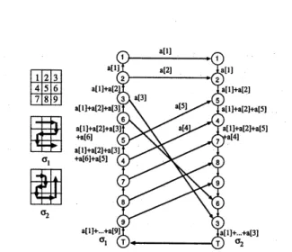
following network-flow algorithm.

A space-filling curve on a matrix can be

re-garded as apermutation of matrix elements. Let

$(\sigma_{\mu}(1), \sigma_{\mu}(2),$

$\ldots,$$\sigma_{\mu}(n^{2}))$ be a permutation

cor-responding to a space-filling $C_{\mu},$$\mu=1,2$

.

Given

an image matrix $a[]$, we wish to compute a

bi-nary matrix $b[]$ of thesame size for which

$\max\{|\sum_{j}^{i}=1(a[\sigma_{\mu}(j)]-b[\sigma\mu(j)])|\}\leq 1$

holds for every $\dot{i},$$1\leq i\leq n^{2}$ and $\mu=1,2$

.

Construct a network as follows (see Fig. 3):

we have two sets of $n^{2}+1$ _nodes, $V_{1}$

$=$ $\{v_{1}(1),v1(2), \ldots , v_{1}(n^{2}+1)\}$ and $V_{2}$ $=$

$\{v_{2}(1), \ldots, v2(n^{2}+1)\}$

.

The first set $V_{1}$ of nodes

are connected in the decreasing order while the

second in the increasing order, that is, we have

arcs $(v_{1}(\dot{i}), v_{1}(i-1))$ for each $i=2,3,$

$\ldots$,$n^{2}+1$

and $(v_{2}(i), v2(i+1))$ for each$\dot{i}=1,2,$$\ldots$,

$n^{2}$

.

Ex-tending $\sigma_{1}$ and $\sigma_{2}$ so that $\sigma_{1}(n^{2}+1)=\sigma_{2}(n^{2}+$

$1)=n^{2}+1$, there is an_obvious $\mathrm{o}\mathrm{n}\mathrm{e}- \mathrm{t}_{0}$-one

corre-spondence between the two permutations $\sigma_{1}$ and

$\sigma_{2}$

.

According to the correspondence we draw an

arc $(v_{1}(\dot{i}), v_{2}(j))$ whenever$\sigma_{1}(\dot{i})=\sigma_{2}(j)$

.

Finally,

we add an arc $(v_{2}(n^{2}+1), v_{1(n^{2}}+1))$.

Arc capacity is defined as follows: Each edge

$(v_{1(\dot{i}),v_{1(i}}-1)),$$2\leq i\leq n^{2}+1$ is associated

with the sum of input values sum1$(\dot{i}-1)=$

$\sum_{j=}^{i1}-a[1\sigma_{1}(j)]$

.

The capacity of the edge is

de-termined by the floor and ceiling of the sum,

i.e., $[\lfloor sum_{1}(\dot{i}-1)\rfloor, \lceil sum1(\dot{i}-1)\rceil]$. For the

sec-ond set ofnodes, each edge $(v_{2}(\dot{i}), v_{2}(\dot{i}+1)),$ $1\leq$

$\dot{i}\leq n^{2}$ is associated with the sum of input

val-ues $sum_{2}( \dot{i})=\sum_{j=1}^{i}a[\sigma_{2}(j)]$

.

The capacity of

the edge is determined by the floor and

ceil-ing of the sum, i.e., $[\mathrm{L}sum2(\dot{i})\rfloor, \lceil sum2(i)\rceil]$

.

The

capacity of the edge $(v_{2}(n^{2}+1), v_{1}(n^{2}+1))$ is

$\ovalbox{\tt\small REJECT}_{78}4561239$

$\ovalbox{\tt\small REJECT}$

$\ovalbox{\tt\small REJECT}^{\circ_{1}}\sigma_{2}$

Figure _{2: A network defined by two space-filling}

curves.

Figure 3: Anetworkdefinedby two binary trees.

$[ \lfloor\sum_{i=}^{n^{2}}1a[i]\rfloor, \lceil\sum_{i=}^{n^{2}}1a[\dot{i}]1]$

.

Any other crossing arc

from $v_{1}(\dot{i})$ to $v_{2}(j)$ is associated with the input

value$a[\sigma_{1}(\dot{i})]=a[\sigma_{2}(j)]$ andits capacity is _$[0,1]$

.

Now, a feasible flow is easily found since

val-ues associated with arcs defined above obviously

satisfy the capacity conditions. Thus, the

well-known integrality theorem implies the existence

of a integer-valued feasible flow. Take any such

flow, and the flow at crossing edges giveabinary

matrixwe wanted.

(ii) Combining Two Binary Structures

Thesame trick worksforadifferent structures.

The network we constructed above has not

hier-archicalstructure. Let usextend thestructure by

replacing each of the two simplepaths with a

bi-narytree structure (see Fig. 3). More concretely,

for a permutation $\sigma_{\mu}$ we construct a binary tree

$T_{\mu}$ with leaves $v_{\mu}(1),$$\ldots$,$v_{\mu}(n^{2})$

.

$\dot{\mathrm{F}}$

or the first set $V_{1}$ we orient the arcs in the

root1 down to the leaves. The arcs in the second

binary tree $T_{2}$ are oppositely directed. We draw

crossingarcsbetween the leaves of$T_{1}$ and$T_{2}$, just

like previously. Eacharcin the trees is associated

with the sum of input values of its descendants

(leaves). Similarly as above, the capacity of each

arc is determined by the floor and ceiling values

of the associated value. Then, those values

as-sociated with arcs define a feasible flow on the

network. Thus, again by the integrality theorem

an integer-valued flow does exist and it gives us

an approximated solution.

(iii) Scaling Algorithm

We have shown apolynomial-time

approxima-tion algorithm for a matrix rounding problem.

However, it does not suffice in practice because

of high timecomplexity of theunderlying flow

al-gorithm. An idea to reduce the time complexity

is to use the integrality of matrix elements.

Al-though we have assumed that each input matrix

element is a real number between $0$ and 1, they

are integers, say 8-bit integers, in an image

ma-trix. Making use of the integrality we can devise

anefficient algorithm.

Assume that each matrixelement is a $k$-bit

in-teger,$0$through$2^{k}-1$

.

Weusethesamestructure

using two binary trees shown in Fig. 3. An idea

is to repeat matrix rounding $k-1$ times until all

the matrix elements become $0$ or 1. Rounding

even

numbers cause no problem. For odd

num-bers we have to choose rounding up or rounding

$\mathrm{d}_{i}\mathrm{o}\mathrm{w}\mathrm{n}$. Our intention here is to balance rounding

ups and roundingdowns. Iftwo odd integers are

adjacent, we should apply different roundings to

them, i.e., rounding up one and rounding down

the other. This idea is generalized as follows: In

the tree$T_{1}$, we mark all leaves having odd values

and their incident arcs. We check each node at

one level up whether the two arcs incident to it

are both marked. If it is the case, we mark the

node and stop. Otherwise, we clime upone more

level in$T_{1}$ and repeat the same check. When we

reach theroot of$T_{1}$, all odd leaves are paired by

paths in $T_{1}$ or connected to the root.

The same process is applied to $T_{2}$

.

Then, we

add the crossing arcs connecting the same

ele-ments in the two sets of leaves. They altogether

form (undirected) cycle(s). Ifwe represent each

such cycle by the integer values

at

thenodesalong

the cycle excluding the duplication,a sequenceof

odd numbers is obtained. Next, we divide each

leaf value by 2. Here, those numbers in the

cy-cles must be rounded to integers. We perform

rounding up and rounding down iteratively along

the sequence obtained above. Of course, there

aretwo different ways of the rounding depending

on whether we start with rounding up or down.

Take any one of the two ways.

We iterate this process $k$ times. Then, all the

resulting leaf values become $0$ or 1. These values

naturally define a binary matrix. Although we

have no space to prove it, the resulting matrix

is one of the feasible flows on the network. This

algorithm is efficient enough.

(iv) $2\cross 2$ neighborhood

In Section 6.2 we claimed that it is NP-hard

to find an optimal rounding ofa real-valued

ma.-.

trix even for the family of $2\cross 2$ neighborhoods.

$\mathrm{H}_{\mathrm{o}\mathrm{W}\mathrm{e}}^{\backslash }\mathrm{v}\mathrm{e}\mathrm{r}$

, with little more constraints we have a

$\dot{\mathrm{p}}$olynomial-time algorithm. The idea is

$\mathrm{t}\dot{\mathrm{h}}\mathrm{e}$

fol-lowing. We regard an image matrix as a checker

board consisting of white and black cells. Then.,

we consider afamily of2 $\mathrm{x}2$ neighborhoods with

white cells at their main diagonals. By the

defi-nition, each cell belongs to at most two (usually

four except for boundary cells) neighborhoods.

Decompose each 2$\mathrm{x}2$ square into two horizontal

pairs and combine them vertically. Then, 2 $\cross 2$

squaresarecombinedhorizontally, andthe

result-ing $2\cross 4$ regions are combined vertically to have $4\cross 4$ regions, etc. Moreover, define costs of arcs

appropriately, sayby $(b-a)^{2}$ where$b$isa flow on

the arc and $a$ is the sum ofthe values in the

de-scendants. Then,we can find anoptimalsolution

in the case ofquadratic costs.

7

Concluding remarks

This paper gives an initial study on the

optimization-based evaluation of digital

halfton-ing algorithms. There are lot of open problems

whichareinteresting from both viewpoints of

the-ory and practice:

(1) For the neighborhood family consisting of

$k\cross k$ squares $(k\geq 2)$, is it always possible to

make $d_{\dot{i}}st(A, B)<c$where$c$is

a

constant strictly

smaller than$k$?

(2) If the answer to (1) is yes, can we design a

condi-tion? (Not seeking for the optimal solution).

One possible candidate is the use of random

space filling curves [4], and perform the

one-dimensional error propagation algorithm along

curves. Ifwe fix a space filling curve, we can

al-ways construct an instance so that $d_{\dot{i}S}t(A, B)>$

$k-\epsilon$; however, it is difficult to construct an

in-stance which performs badly for many randomly

chosen fillingcurves simultaneously.

(3) Are there any good approximation algorithm

which has a theoretical performance ratio?

(4) Find a very good neighborhood family and

error function to evaluate the quality of

digi-tal halftoning in practice. If such a framework

is firmly established, modern heuristic methods

can be $\mathrm{P}^{\mathrm{r}\mathrm{o}\mathrm{b}\mathrm{a}\mathrm{b}1}.\mathrm{y}$ applied to have a good digital

halftoning.

References

V. T. S\’os, Colloq. Math. Soc. J’anos Bolyai

10, pp.91-108.

[8] B. Bollob\’as, Combinatorics, Cambridge

Uni-versity Press, 1986.

[9] J. Beck and V. T. S\"os, Discrepancy Theory,

in Handbook

_of

Combinatorics Volume II,

(ed.R.Graham, M. Gr\"otschel, and LLova’sz)

1995, Elsevier.

[10] R. W. Floydand L. Steinberg: “An adaptive

algorithm for spatialgrayscale,” SID $7\mathit{5}D_{\dot{i}-}$

gest, Society

_{for Information}

Display, (1975)

pp.36-37.

[11] M. R. Garey and D. S. Johnson: Computers

and Intractability: A guide to theory

_of

NP

hardness, Feeman and Company, 1979.

[12] D. E. Knuth: “Digital halftones by dot

dif-fusion,” ACM $r_{\mathrm{b}\mathrm{a}\mathrm{n}\mathrm{s}}$

.

Graphics, 6-4 (1987),

pp.245-273.

[1] R. Ahuja, T. Magnanti, and J. Orlin,

Net-work Flows, Theory Algorithms and

Appli-cations, Princeton Hall,

[2] T. Asano, T. Matsui, and T. Tokuyama:

“On the Complexities oftheOptimal

Round-ing Problems of Sequences and Matrices,”

Proc. 7th Scandinavian Workshop on

Algo-rithm Theory, pp.476-489, Bergen, Norway,

July 2000.

[3] T. Asano: “Digital Halftoning Algorithm

Based onRandomSpace-Filling Curve,”

IE-ICE $r_{\mathrm{b}\mathrm{a}\mathrm{n}\mathrm{s}}$

.

on Fundamentals, Vol.E82-A,

No.3, pp.553-556, March 1999.

[4] T. Asano, N. Katoh, H. Tamaki, and T.

Tokuyama: “Convertibility among grid

fill-ingcurves,” Proc. ISAAC98, SpringerLNCS

1533 (1998), pp.307-316.

[5] T. Asano, D. Ranjan and T. Roos: “Digital

halftoning algorithms based onoptimization

criteria and their experimental evaluation,”

IEICE Trans. Fundamentals, Vol. E79-A,

No. 4, pp.524-532, Apri11996.

[6] B. E. Bayer: “An optimum method for

two-level rendition of continuous-tone

pic-tures,”

_Conference

Record, IEEE

Interna-tional

_Conference

on Communications, 1

(1973), $\mathrm{p}\mathrm{p}.(26- 11)-(26- 15)$

.

[7] Z. Baranyai, “On the factorization of the

complete uniform hypergraphs”, in

_Infinite

and Finite Sets, eds. A. Hanaj, R. Rado and

[13] J. O. Limb: “Design of dither waveforms for

quantizedvisual signals,” Bell Syst. Tech. J.,

48-7 (1969), pp. 2555-2582.

[14] B. Lippel and M. Kurland: “The effect

of dither on luminance quantization of

pic-tures,” IEEE Trans. Commun. Tech.,

COM-19 (1971), pp.879-888.

[15] M. Minoux: “Solving Integer Minimum

Cost Flows with Separable Cost Objective

Polynomially,” Mathematical Programming

Study 26 (1986) pp.237-239.

[16] M. Miyahara, K. Kotani, and V.R. Algazi:

“Objective Picture Quality Scale (PQS) for

Image Coding,” IEEE Trans. on

Communi-cations, 46, 9, pp.1215-1226, Sept. 1998.

[17] V. Ostromoukhov, R.D. Hersh, and I.

Amidror: “RotatedDispersedDither: aNew

Technique for Digital Halftoning,” Proc. of

SIGGRAPH ’94, (1994) pp.123-130.

[18] R. Ulichney: Digital halftoning, MIT Press, 1987.

[19] L. Velho and de M. Gomes: ”Digital

Halfton-ing with Space FillHalfton-ing Curves,” Proc.

ofSIG-GRAPH ’91, (1991) pp.81-90.

[20] Y. Zhang and R. E. Webber: ”Space

Diffu-sion: AnImprovedParallelHalftoning

Tech-nique Using Space-Filling Curves,” Proc. of