MEASUREMENT OF TECHNOLOGICAL PROGRESS IN TERMS OF LEARNING RATES AN ANALYSIS OF THE MEXICAN MANUFACTURING INDUSTRY
GONZALEZ CORTEZ JOSE LUIS 52109609
A THESIS SUBMITTED TO THE GRADUATE SCHOOL OF MANAGEMENT IN PARTIAL FULFILLEMENT OF THE REQUIREMENTS FOR THE DEGREE OF
MASTER IN BUSINESS ADMINISTRATION
SUPERVISOR BEHROOZ ASGARI
GRADUATE SCHOOL OF MANAGEMENT RITSUMEIKAN ASIA PACIFIC UNIVERSITY
BEPPU, OITA, JAPAN
STATEMENT OF AUTHENTICITY
By virtue of submitting this thesis, I certify that except where due acknowledgement has been made, the work is of my own; and the research has not been submitted previously, in whole or in part, to qualify for any other academic award. Research work carried out by a third party is acknowledged; and, ethics procedures and guidelines have been followed.
Gonzalez Cortez Jose Luis
July, 2011
Measurement of Technological Progress in Terms of Learning Rates
An Analysis of the Mexican Manufacturing Industry
ABSTRACT
The development and advancement of a manufacturing industry encompasses specialization changes over time shifting from low tech-labor intensive industries to high tech-capital intensive industries as the ultimate stage. The stock of knowledge and technological capabilities determine the technological progress of an industry. This thesis performs an analysis of the Mexican manufacturing subsectors and estimates their progress ratios or learning coefficients through a linear and a cubic model integrated into a neoclassical production function. The study seeks to determine whether Mexico is moving from labor intensive to capital intensive industries, and identify the subsectors that the country should prioritize.
It is found that there are three main patterns of technological learning among different industries: a convex learning path with a forgetting all the time or learning at some beginning periods but forgetting afterwards, a concave learning path with forgetting after beginning periods but learning afterwards, and a concave learning path with forgetting all the time. The Machinery industry is located in a forgetting stage showing a detriment performance over time, but the Railroad and Transport Equipment subsector shows an exceptional technological learning and assimilation capacity. In order to sustain industrial and economic growth, Mexico should prioritize Mid-Low and Mid-High Tech industries that show learning potentials, and adjust its technology policy structure to reverse the High Tech industry performance. Policies should be enforced to support, and do not neglect, the Food industry which remains very competitive with a high assimilation capacity.
Keywords: Learning Curve, Progress Ratio, Technological Progress, Mexican Manufacturing Industry.
I List of Figures
Fig. 1. Mexico GDP Value and Growth Rate. ... 2
Fig. 2. FDI in Mexico by Sector “Percentage Contribution”. ... 5
Fig. 3. Mexico: Import, Export and FDI (US Dollars at current prices and current exchange rates in millions). ... 6
Fig. 4. GDP Contribution by Sector. ... 7
Fig. 5. Exports Participation of Non-Oil Related Sectors in Mexico. ... 8
Fig. 6. Progress Ratio Values for the Food Industry (Low Tech). ... 32
Fig. 7. Progress Ratio Values for the Chemical Industry (Mid-High Tech). ... 33
Fig. 8. Progress Ratio Values for the Non-Metallic Industry (Mid-Low Tech). ... 34
Fig. 9. Progress Ratio Values for the Basic Metals Industry (Mid-Low Tech). ... 34
Fig. 10. Progress Ratio Values for the Machinery Industry (High Tech). ... 35
Fig. 11. Progress Ratio Values for the Textile Industry (Low Tech). ... 36
Fig. 12. Progress Ratio Values for the Wood Industry (Low Tech). ... 37
Fig. 13. Progress Ratio Values for the Paper Industry (Low Tech). ... 37
Fig. 14. Manufacturing Production Contribution by Technological Intensity. ... 39
Fig. 15. Progress Ratio Values for the Machinery and Equipment Industry (Medium-High Tech). .... 44
Fig. 16. Progress Ratio Values for the Computing Machinery, Communications Equipment, Medical, Precision and Optical Industry (Medium-High Tech). ... 44
Fig. 17. Progress Ratio Values for the Electrical Machinery and Apparatus Industry (Medium-High Tech). ... 45
Fig. 18. Progress Ratio Values for the Fabricated Metal Products Industry (Medium-Low Tech). ... 45
Fig. 19. Progress Ratio Values for the Railroad and Transport Equipment Industry (Medium-High Tech). ... 46 Fig. 20. Manufacturing Production Contribution of Industries grouped into the Machinery Industry. 46 .
II List of Tables
Table 1 Trade Liberalization in Mexico ... 2
Table 2 Mexico Total Trade in Merchandise and Services... 3
Table 3 Mexico’s Foreign Direct Investment Distribution by Economic Sector ... 5
Table 4 Researchers Focusing on the Learning Curve ... 11
Table 5 Classification Scheme of Technological Change ... 17
Table 6 Progress Ratio Value Interpretation ... 18
Table 7 Mexican Sub-Sector Classification “Technological Intensity” ... 21
Table 8 Data Processing (Linear Model) Sub-Sector: Wood ... 26
Table 9 Linear Model Regression Results and Progress Ratio Value ... 26
Table 10 Progress Ratio Estimates by Sub-Sector (1988-2008) ... 27
Table 11 Data Processing (Cubic Model) Sub-Sector: Wood ... 28
Table 12 Cubic Model Regression Results ... 28
Table 13 Progress Ratio Estimates by Manufacturing Sub-Sector ... 29
Table 14 Average Progress Ratio Values Before and After NAFTA ... 31
Table 15 Industry Participation in the Total Manufacturing Production Value ... 38
Table 16 Industry Production Contribution Before and After NAFTAa ... 38
Table 17 Patterns of Technological Learning Over Time... 40
III Notations
Altex Program for High Export Oriented Companies
At Stock of technology at time t
c1 unit production cost at time 1
CPI Consumer Price Index
ct Unit production cost in time t
d Progress ratio or learning level
FDI Foreign Direct Investment
GATT General Agreement on Tariffs and Trade
GDP Gross Domestic Product
IMF International Monetary Fund
INEGI Mexican Statistics, Geography and Information Bureau
ISI Import Substitution Industrialization
ISIC International Standard Industrial Classification
K Capital
L Labor
MC Marginal Cost
NAFTA North America Free Trade Agreement
OECD Organization for Economic Cooperation and Development
Pitex Temporary Importation Program for Exportation
Q Production Value Added
u1 Direct-hours required to produce the 1st unit of a product
WB World Bank
Xt Cumulative Production at time t
yt Direct-hours required to produce the xth unit of a product
IV TABLE OF CONTENTS
1. Introduction ... 1
1.1. Mexican Economy Performance in the last three decades... 1
1.2. Trade Liberalization and Industrialization Process ... 2
1.2.1. Phase 1) Economic reforms (1980-1985) ... 3
1.2.2. Phase 2) Adherence to the GA TT (1986)... 4
1.2.3. Phase 3) North American Free Trade Agreement (1994) ... 5
1.3. Mexican Manufacturing Industry Development ... 6
1.4. Research Purpose and Objectives... 8
2. Literature Review ... 10
2.1. Learning Process and its Economic Implication ... 10
2.2. Learning Curve Theory ... 11
2.3. Emergence of the Experience Curve concept ... 14
2.4. S-Curve Models ... 14
2.5. Technological Capability and Technological Progress ... 16
2.6. Hypothesis ... 19
3. Research Methodology ... 20
3.1. Data Collection ... 20
3.2. Data Processing ... 20
3.3. Sub-Sectors Classification According to their Technological Intensity ... 20
3.4. The Traditional Linear Model Construction ... 21
3.5. The Cubic Model Construction ... 23
3.5.1. Learning elasticity estimation ... 25
3.6. The Model Computation ... 25
4. Results and Discussion ... 30
4.1. The Linear Model versus the Cubic Model... 30
4.2. Sub-Sectors in Learning Situations ... 32
4.3. Subsectors in Forgetting Situations ... 34
4.4. Manufacturing Subsectors by Technological Intensity ... 38
4.5. Patterns of Technological Learning Level ... 40
4.5.1. Convex Learning Path with Minimum ... 40
4.5.2. Concave Learning Path with Maximum ... 41
4.5.3. Concave Learning Path with No maximum ... 41
4.6. The Contributing Factors of Technological Learning ... 41
V
6. Conclusions and Policy Implications ... 47
Bibliography ... 49
Appendix A Manufacturing Industry Classification Before and After 2003... 52
Appendix B Exchange Rate “Mexican Pesos per US Dollar” ... 53
Appendix C Mexico Consumer Price Index 2005=100 ... 54
Appendix D Classification of Industries based on Technology Intensity (OECD) ... 55
Appendix E Production, Remunerations and Value Added by Sector (Current Mexican Pesos)... 56
Appendix F Data Processing by Subsector (Linear Model) ... 61
Appendix G Data Processing by Subsector (Cubic Model) ... 71
1 1. Introduction
1.1. Mexican Economy Performance in the last three decades
Mexico’s macroeconomic policies have changed over the last 60 years. Prior to the 1970’s the Mexican economy was directly influenced by the government who had a direct control of the economic development through state owned companies and by implementing strict controls in the internal market and international trade, but early in the 1980’s Mexico implemented several “neoliberal policies” following the International Monetary Fund and the World Bank recommendations (Calva, 2004).
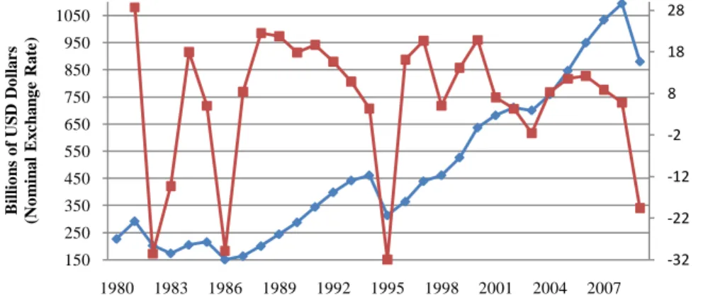
In the last three decades (1980-2010) the Mexican Gross Domestic Product shows an overall continuous growth with drastic decreases early in the 1980’s due to extremely high inflation rates as a result of poor macroeconomic policies and an excessive external debt. From 1986 to 1993 Mexico’s GDP showed a sustained growth as depicted in Figure 1. In 1994 Mexico went through a huge economic turndown that influenced South American economies and its economic effect in the region is well known as the tequila effect. In 2009 the Mexican GDP decreased by 19.5 percent as shown in Figure 1 due to the recent global economic recession.
Calva (2004) argues that the Mexican economic growth during 1983-2002 is the result of short term macroeconomic policies implemented by the Mexican government: a) drastic reduction in government expenditure (from 11.9% in 1982 to 8.7% in 1988 as a percentage of GDP), and public investment (from 10.4% to 4.9% in the same period); b) good prices increase and price increases in government services that reduced the purchasing power; c) reduction in salaries by implementing salary ceilings; and d) reduction in money supply and credits (Calva, 2004).
The Mexican Gross Domestic Product shows a sustained growth after 1995 (Figure 1), with a 381 percent growth from 1980 to 1998, as a result of macroeconomic policies implemented since the 1980’s and the Trade Liberalization Process that culminated in the North America Free Trade Agreement (NAFTA) in 1994. This trade liberalization process had impacted the whole Mexican economy and has forced the re-allocation of resources in different sectors and industries (Cardero & Aroche, 2008).
2
Fig. 1. Mexico GDP Value and Growth Rate.
Source: UNCTAD, UNCTADstat
1.2. Trade Liberalization and Industrialization Process
Mexico determined to grow under a closed economy after the World War II by implementing several import restrictions and trade policies early in the 1950’s (Hernadez Laos, 2005), and afterwards decided to move towards an open economy throughout a trade liberalization process which began from 1985 going forward (Esquivel & Rodriguez Lopez, 2003). Mexico implemented macroeconomic policies that let the country move from a closed economy to an open economy in the last decades.
The major trade liberalization process in Mexico (initiated in 1985) can be divided into three main stages as shown in Table 1, a similar classification that appears in a research conducted by Esquivel and Rodriguez Lopez (2003): Economics reforms that were initiated early in the 1980’s by recommendations of the International Monetary Fund (IMF) and the World Bank, Mexico’s adherence to the General Agreement on Tariffs and Trade (GATT) in 1986, and the North America Free Trade Agreement that came into effect in 1994.
Table 1 Trade Liberalization in Mexico Phase 1 1980 Phase 2 1986 Phase 3 1994
Economic reforms (IMF and WB) General Agreement on Tariffs and Trade (GATT) NAFTA Agreement US-Canada-Mexico Import Substitution Industrialization (ISI). Closed Economy
Market/Export oriented policy Semi-Open Economy
Export oriented policy Open Economy Import quotas decreased from
100% to 31%
Max tariff from 100% to 25% Maquila Program
New FDI law was enacted FDI increased 1900% from 1994-2008 -32 -22 -12 -2 8 18 28 150 250 350 450 550 650 750 850 950 1050 1980 1983 1986 1989 1992 1995 1998 2001 2004 2007 Bill io n s o f U S D D o ll a r s (N o m in a l Ex c h a n g e R a te ) GDP Value GDP Growth Rate %
3 1.2.1. Phase 1) Economic reforms (1980-1985)
Mexico underwent a debt crisis in the early 1980’s, and international investors refused loans to the Mexican government. Mexico had no other option but to request support to the IMF and the World Bank that released financial support under strict conditions aimed to reform its macroeconomic policies, therefore, Mexico implemented several macroeconomic policies of adjustment and stabilization which created high inflation rates averaging 94.6 percent per year between 1982-1987 (Hernadez Laos, 2005).
Table 2 Mexico Total Trade in Merchandise and Services
YEAR Exportsa Importsa FDIa
GDP
Percapitab YEAR Exportsa Importsa FDIa
GDP Percapitab 1980 18,031 22,144 1,910 3,306 1995 79,542 75,858 4,405 3,423 1981 23,307 28,462 2,522 4,154 1996 96,000 93,674 10,792 3,905 1982 24,055 17,742 3,115 2,831 1997 110,431 114,847 18,993 4,628 1983 25,953 12,476 1,326 2,382 1998 117,460 130,948 28,856 4,779 1984 29,101 16,691 1,501 2,760 1999 136,391 148,648 28,578 5,371 1985 26,757 19,116 1,418 2,846 2000 166,368 182,702 32,779 6,397 1986 21,804 17,573 317 1,960 2001 158,547 176,185 22,457 6,761 1987 27,600 19,697 1,169 2,083 2002 160,682 176,607 16,590 6,969 1988 30,691 29,402 2,805 2,502 2003 165,396 178,503 10,144 6,788 1989 35,171 36,400 1,130 2,988 2004 189,084 206,623 18,146 7,273 1990 40,711 43,548 989 3,453 2005 213,891 231,821 15,066 8,014 1991 42,688 52,315 1,102 4,055 2006 250,441 268,169 18,822 8,887 1992 46,196 65,050 2,061 4,600 2007 272,055 296,578 34,585 9,484 1993 51,886 68,439 1,291 5,005 2008 291,827 325,157 45,058 9,964 1994 60,882 83,075 2,150 5,126 2009 229,683 246,104 25,949 7,921 a
US Dollars at current prices and current exchange rates in millions (exports, imports and FDI)
b
US Dollars at current prices and current exchange rates per capita Source: UNCTAD, UNCTADstat
Trade liberalization was part of the policies implemented during this period, dismantling the protectionism by reducing import quotas from 100 percent of imports in 1982 to 30.95 percent in 1985 (Hernadez Laos, 2005). Contrary to expectations of an increase in imports, the data shows that in fact Mexico showed a 14 percent reduction in its total imports between 1980 and 1985 as shown in Table 2, and on the contrary exports increased 48 percent in the same period. Foreign Direct investments decreased by 25 percent due to economic uncertainty especially because of high inflation rates and restrictions to foreign direct investments before 1984.
4
A new law for FDI was enacted in 1984 that allowed investments in export-oriented, capital-intensive and technologically advanced sectors that attracted FDI in the following years (Esquivel & Rodriguez Lopez, 2003).
In 1983 Mexico initiated a privatization process for the majority of the state-owned companies in order to promote competitiveness, productivity, technology transfer and eliminate the burden on non-profitable state-owned companies. The Mexican government established the bases to transition to an open economy which had an impact on its manufacturing industry in the forthcoming years.
1.2.2. Phase 2) Adherence to the GA TT (1986)
In 1986 Mexico joined the GATT and agreed to eliminate several import/export controls. Protection levels were dramatically reduced during the period of 1985-1993. Domestic product covered by import permits decreased from 92.2 percent to 16.5, maximum tariff from 100 percent to 25 percent, and imports subject to permits from 35.1 percent to 21.5 percent (Esquivel & Rodriguez Lopez, 2003).
In 1986 Mexico implemented a program that allowed companies to process temporary imports for raw materials, equipment and machinery bounded to manufacture products for exportation under the Pitex program (Temporary Importation Program for Exportation – Programa de Importacion Temporal para la Exportacion). In 1987 Mexico launched a new program for high export-oriented companies that provided additional administrative advantages under the Altex program (Program for High Export Oriented Companies – Programa para Empresas Altamente Exportadoras), and in 1993 a law that regulates the foreign trade transactions was enacted. At the end of this period, only 3 sectors kept rigorous commercial restrictions: agriculture, oil refining and transport equipment (Esquivel & Rodriguez Lopez, 2003). The FDI law was reformed in 1993 to foster a more competitive environment for foreign and domestic investments (Vazquez Galan, 2009).
Pitex and Altex programs and the new FDI scheme played an important role in promoting investments in the manufacturing industry. During this period 1986-1993, the FDI increased 300 percent as shown in Table 2; exports and imports increased 137 percent and 290 percent
5
correspondingly. Mexico initiated its insertion into the international trade arena and became an attractive market for FDI as shown in Figure 1 and Table 2.
Table 3 Mexico’s Foreign Direct Investment Distribution by Economic Sector Definition/Year 1980 1985 1990 1995 2000 2002 2004 2005 2006 2007 2008 2009 2010
Industry 79.2 67.4 32.0 58.7 57.4 41.2 59.6 47.2 49.9 45.5 30.0 36.1 59.7
Services 8.1 25.2 59.2 28.3 27.6 49.6 34.1 40.0 44.7 43.2 44.7 49.9 22.8
Retailing 7.3 6.3 4.6 12.1 13.6 7.8 5.5 12.0 3.3 5.2 7.1 9.0 14.2
Extraction 5.3 1.0 2.5 0.9 0.9 1.1 0.8 0.8 2.0 5.6 18 4.9 3.3
Agriculture and livestock 0.1 0.0 1.6 0.1 0.5 0.4 0.1 0.0 0.1 0.5 0.1 0.1 0.0
Total Percentage 100 100 100 100 100 100 100 100 100 100 100 100 100
Source: Vazquez Galan (2009) and Mexican Economy Bureau
The implementation of policies and institutions to stimulate trade was a key factor for the attraction and allocation of FDI primarily in the Mexican industry sector as illustrated in
Figure 2. In 1980, as shown in Table 3, 79.2 percent of the total FDI was concentrated in the
Mexican industry sector and in 1985 67.4 percent.
Fig. 2. FDI in Mexico by Sector “Percentage Contribution”.
Source: Vazquez Galan (2009) and Mexican Economy Bureau
1.2.3. Phase 3) North American Free Trade Agreement (1994)
In 1990 Mexico initiated negotiations with Canada and the US to sign the North America
Free Trade Agreement that came into effect on January 1st, 1994. During the first year of the
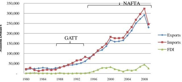
agreement more than 80 percent of all trade restrictions were eliminated (Hernadez Laos, 2005). Figure 3 shows a dramatic growth of trade (imports and exports) that had continued over time with a decrease in 2009 due to the worldwide financial crisis. Exports show a 379 percent growth between 1994 and 2008, imports 290 percent growth and FDI 1900 percent increase during the same period.
0 10 20 30 40 50 60 70 80 1980 1995 1998 2001 2004 2007 2010 P e r c e n tage Industry Services Retailing Extraction
6
NAFTA stimulated capital inflows that have been concentrated in the industry sector; as an average over 50 percent every year has been allocated to this sector as shown in table 3. This important allocation of FDI in this sector has contributed to the increase in the Mexican manufacturing industry activity. In addition, Mexico also implemented changes in its transportation system aligned with the trade liberalization process, privatizing the seaports and the railway system in 1993 and 1997 respectively in order to promote an efficient transportation system.
Fig. 3. Mexico: Import, Export and FDI (US Dollars at current prices and current exchange rates in millions).
Source: UNCTAD, UNCTADstat
1.3. Mexican Manufacturing Industry Development
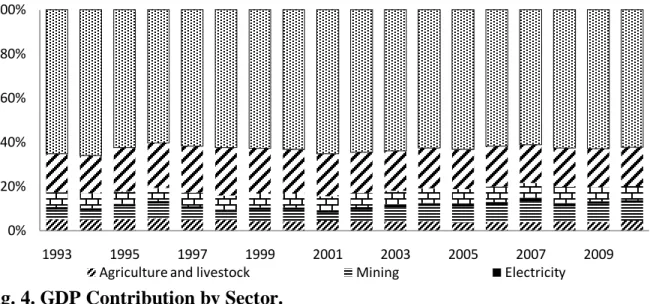
The contribution of different sectors (Agriculture and Livestock, Mining, Electricity, Construction, Manufacturing Industry, and Commerce and services) to the Mexican GDP in the last two decades, depicted in Figure 4, has remain the same with a slight increase in the Mining sector. It is observed that manufacturing industry’s contribution to the Mexican GDP has remained the same, yet this does not imply that the production value and total exports have remained stagnated, but it implies that the Mexican economy shows a sustainable growth in all sectors in the last two decades.
-50,000 100,000 150,000 200,000 250,000 300,000 350,000 1980 1984 1988 1992 1996 2000 2004 2008 M il li o n D o ll ar s Exports Imports FDI GATT NAFTA
7
In the last two decades, especially after the intervention of the IMF and WB in the Mexican macro policies early in the 1980’s, the Mexican industry and international trade policies have been aligned to the promotion of the manufacturing industry exports (CEFP, 2004).
Fig. 4. GDP Contribution by Sector.
Source: INEGI
The Mexican manufacturing industry’s contribution to the total exports of non oil related exports has significantly increased from around 50 percent in the 1980’s to above 90 percent in the last decade as shown in Figure 5. The manufacturing industry has an active participation in the Mexican exports, nevertheless when analyzing its contribution to the total GDP; it is observed that its contribution has remained the same since 1993 at around 18 percent. In spite of its 18 percent contribution to the total GDP, the manufacturing industry is considered the main contributor of the economic growth and industry development in the country (CEFP, 2004).
Several studies have shown that from 1985 and predominantly after 1995, Mexico is listed among the main 10 countries with high export participation in the global market (Moreno, Santamaria, & Rivas, 2009).
Given the fact that the manufacturing industry is the main contributor to the Mexican exports and imports, it is important to analyze its evolution in order to determine its current industrial specialization. In terms of the sub-sectors’ contribution to the manufacturing industry, some industries show a decreasing participation such as textiles, wood, paper and some others show an expansion such as metallic products and machinery and equipment (Cardero & Aroche, 2008). 0% 20% 40% 60% 80% 100% 1993 1995 1997 1999 2001 2003 2005 2007 2009
8
Fig. 5. Exports Participation of Non-Oil Related Sectors in Mexico.
Source: Mexican Economy Bureau
The Mexican manufacturing industry depicts a continuous growth in terms of exports with an important contribution to the GDP although its contribution level remains at around 18 percent, but the question is whether all the sub-sectors are performing well or if this continuous growth relies on some sub-sectors only.
1.4. Research Purpose and Objectives
The Mexican manufacturing sector, as reviewed, shows a continuous growth and its high contribution in the total non-oil related exports of the Mexican economy raises the concern whether different sub-sectors that integrate it are actually performing well or whether the whole good performance of the manufacturing industry relies on certain sub-sectors only.
The aim of this research is to conduct an analysis of all the sub-sectors that integrate the Mexican manufacturing industry and determine the following:
1. Which manufacturing industries should Mexico focus on? 2. Is Mexico progressing in High Tech manufacturing industries?
3. Which changes should Mexico implement in its manufacturing industry strategy to enhance its growth?
0 10 20 30 40 50 60 70 80 90 100 1980/01 1986/01 1992/01 1998/01 2004/01 2010/01 P e r c e n tage MFG Industry
Agriculture & Livestock Extraction
9
This research identifies the manufacturing subsectors with good and poor performance, and also assesses whether Mexico is moving from labor-intensive to capital-intensive sub-sectors.
This assessment is carried out by measuring the technological progress in terms of learning rates in each sub-sector, and by identifying different levels of knowledge accumulation among them.
10 2. Literature Review
2.1. Learning Process and its Economic Implication
Several studies have demonstrated that the increased efficiency in processes is explained by the increased familiarity with the routine of such processes. In other words, as a recurrence of
a process occurs in t1, there is an accumulation of knowledge that leads to a better
performance of such process in t1+n. This accumulation or acquisition of knowledge is what
has been termed “learning” (Arrow, 1962). This particular role of knowledge accumulation in the increase of productivity was originally observed and studied by T.P Wright in 1936 in the production of airframes, concluding that the required labor-hours spent in the production of an airframe is a decreasing function of the total number of airframes of the same type previously produced.
Learning by Doing refers to the process by which production costs are reduced as experience is accumulated over time (Hornstein & Peled, 1997), and this knowledge accumulation can be depicted by a learning curve that shows the relationship of outputs and inputs, and most important how learning by doing induces improvements in the output performance over time. Different studies have termed learning curves as manufacturing progress function, cost-quality relationship, cost curve, product acceleration curve, improvement curve, performance curve, experience curve, and efficiency curve (Belkaoui, 1986).
As a person/worker becomes accustomed to, and experienced in, the process that he or she performs, the worker progressively learns how to do tasks more efficiently and quickly. The experience gained by the worker is positively correlated to the cumulated amount of output produced or activity performed (Jackson, Introduction to Economics: Theory and Data, 1982).
Arrow (1962) in his seminal work “Economic Implications of Learning-by-Doing” concluded that learning happens when attempting to solve a problem.
1
11 2.2. Learning Curve Theory
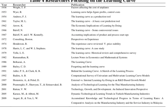
The learning curve phenomenon has been of interest to researchers for the last 80 years as shown in Table 4. The initial observation of the learning curve is attributed to T.P Wright in 1936 when conducting a research of factors affecting the cost of airplanes finding that learning contributes to the reduction in labor-hours spent in the production of an airframe. In 1954 Andress, F.J conducted a research on the learning curve as a production tool focusing on the role of the direct labor in the learning system (Adler & Clark, 1991).
Arrow (1962) studied the economic implications of Learning-by-Doing. Baloff (1966) undertook a research to broaden the application of the learning curve in capital-intensive industries, introducing a learning model for a variety of industries and reviewed some empirical results (Baloff, 1966). Baloff and Kenelly (1967) argued that a learning model should be taken into consideration when estimating the productivity path of a start-up process, and that productivity increases have accounting implications for capital budgeting and project evaluation.
Table 4 Researchers Focusing on the Learning Curve
Year Researcher Publication
1936 1953 1954 1961 1962 1966 1967 1972 1974 1978 1979 1982 1986 1989 1991 1992 1997 2000 2001 2005 2009 Wright, T. P. Wyer, R. Andress, F. J. Taylor, M. L. Arrow, K. Baloff, N.
Baloff, N. and J. W. Kennelly. Consulting, Boston. Henderson, B.
Harris, L. C. and W. L Stephens. Yelle, L. E.
Ramanathan, R. Belkaoui, A. Bailey, C. D.
Adler, P. S., & Clark, K. B. Badiru, A. B.
Hornstein, A., & Peled, D.
Pramongkit, P., Shawyun, T., & Sirinaovakul, B. Ruttan, V. W.
Karaoz, M., & Albeni, M. Asgari, B., & Yen, L. W.
Factors affecting the cost of airplanes Learning curve helps figure profits, control costs The learning curve as a production tool The learning curve - A basic cost prediction tool The Economic Implications of Learning by Doing The learning curve - Some controversial issues Accounting implications of product and process start-ups Perspectives on Experience
The experience curve reviewed: V. price stability The learning curve: A case study
The learning curve: Historical review and comprehensive survey Lecture Notes in Economics and Mathematical Systems The Learning Curve
Forgetting and the learning curve
Behind the Learning Curve: A Sketch of the Learning Process
Computational Survey of Univariate and Multivariate Learning Curve Models External vs. Internal Learning-by-Doing in an R&D Based Growth Model Analysis of Technological Learning for the Thai Manufacturing Industry Technology, Growth, and Development. An Induced Innovation Perspective Dynamic Technological Learning Trends in Turkish Manufacturing Industries
Accumulated Knowledge and Technological Progress in Terms of Learning Rates: A Comparative Analysis on the Manufacturing Industry and the Service Industry in Malaysia
12
A learning curve can be defined as a function which relates performance to experience (Jackson, 1998). Learning curves demonstrate that improvements in the output performance of any process, induced by knowledge accumulation follows an S shape over time, which
leads to the conclusion that at some point in tn the learning effects are bounded or that
learning eventually ceases (Hornstein & Peled, 1997).
There are five main characteristics of the learning curves described in Hornstein and Peled’s research that can be considered as the “stylized facts” of Learning-by-Doing
a) Learning has a significant effect on efficiency
Learning by doing has an increasing gradual effect on the performance and rapidness of a specific task. An operator in a production line performing a pad printing operation for a plastic component for the first time, needs more time to achieve this activity versus an operator that has been in this position for a week. As the operator performs the same pad printing operation repetitively, the amount of time to execute this activity decreases over time, leading to a better efficiency in this particular task. As learning happens (accumulation of knowledge) efficiency increases.
b) Learning increases as a function of production volume
Learning can be maximized with a continuous mass production of a specific component or with a continuous performance of the same process. Taking the previous example, accumulation of knowledge in the pad printing operation will be maximized if there is a continuous and interrupted pad printing operation of the same kind of plastic component and environment. If this pad printing operation happens only once a week (just 1 day), there will be knowledge accumulation but not at the same level if this pad printing operation is performed every single day of a month calendar.
c) The scope of learning is bounded
Accumulation of knowledge for a particular unchanged process cannot continue perpetually and the rate of such knowledge accumulation changes over time following the S-Curve shape. Different studies have come to the conclusion that learning does not continue indefinitely, cost improvements correlated by the accumulation of knowledge eventually stop or falls to very low rate that in practice are ignored (Hall & Howell, 1985).
13
d) There is an important component to learning which is firm-specific
There is an empirical regularity in manufacturing industries where the unit cost of the second
unit is 80 percent of those of the nth unit; however, this learning elasticity shows some
variation across industries or even within the same industry, leading to the conclusion that accumulation of knowledge or the stock of knowledge achieved is firm-specific (Hornstein & Peled, 1997). According to Grubler (1998) learning varies from industry to industry, from tech to tech, and from firm to firm. High labor industries such as the manufacturing industry show high learning elasticity rates versus low labor industries such as the tourism industry.
e) The experience effect on the development of new goods is more modest than its impact on efficiency
Hornstein and Peled (1997) consider three versions of the learning process, but these can be classified as two main versions which are the following: endogenous learning in which the stock of knowledge is explained within the model and exogenous learning in which the stock of knowledge comes from the outside of the model and it is not explained by the model itself.
Several papers have documented the evolution of the learning curve models, from univariate models to more complex multivariate models. Typical learning curves correlate production cost and cumulative production outputs based on the effect of learning (Badiru, 1992). T.P Wright (1936) found that a given operation is subject to a 20% productivity improvement each time the production quantity doubles.
Conventional univariate learning curves express a dependent variable (e.g, total production) in terms of a particular independent variable such as labor cost, investment, etc. According to Badiru (1992) the most famous univariate models include: the log-linear model, the S-curve, the Stanford-B model, DeJong’s learning formula, Levy’s adaptation formula, Glover’s learning formula, Pegel’s exponential function, Knecht’s upturn model, Yelle’s product model, and multiplicative Power Model.
Realistic analysis of productivity gains have enforced the extension and modifications of conventional learning curves since there are numerous factors that can influence how quickly and how distant, and how well a worker learns within a given time horizon and environment. Multivariate models have not been well studied perhaps due to the complexity of implementing the models for practical productivity assessments (Badiru, 1992).
14
A very simple model can be reduced to a bivariate model of the form: Y = βo X1β1 X2β2
Where Y is a measure of cost and X1 and X2 are the independent variables (β1 and β2 learning
rates). With this very simple bivariate model, it is possible to obtain accurate estimates of the effects of two variables involved. Multivariate models are more robust and help account for more of the available data (Badiru, 1992).
2.3. Emergence of the Experience Curve concept
The experience curve phenomenon was developed by the Boston Consulting Group (1960-1970’s), looking at the total cost and widening the inputs to the learning system. The experience curve, contrary to the learning curve, takes into consideration all possible inputs in a production process to find a relationship between one of many, substitutable inputs and cumulative output (OECD, Experience Curves for Energy Technology Policy, 2000).
The BCG applied to the total cost of a product, including different learning means such as research and development, economies of scale, and other cost factors. Additionally, the concept was applied not only within a single company or process, but also to entire industries (Sark Van, 2008).
2.4. S-Curve Models
a) The Log-Linear Model
Since the publication of the first article formulating the theory of learning curves in 1936, various models and geometric versions have been proposed, but the log-linear model has been and still is the most used model. The log-linear model or constant percentage model states that the improvement in productivity is fairly constant as output increases (Belkaoui, 1986).
Its mathematical function is described as follows: yt = u1 Xtα where:
yt = the number of direct-hours required to produce the xth unit
u1 = the number of direct-hours required to produce the 1st unit
Xt = the cumulative unit number
15
The relationship between the cumulative average direct-labor hours and the cumulative units of production plotted on a logarithmic scale follows a straight line declining rate, but it is extremely important to highlight that the learning elasticity (α) is a constant figure over the whole period of analysis. The calculation of the learning elasticity is straight forward when applying a logarithmic approach and linear regression analysis.
The search of other models is given the fact that the linear model does not always provide the best fit in all situations.
b) The S-Curve
The S-type function has the shape of the cumulative normal distribution function for the start-up curve and the shape of an operating characteristic function for the learning curve. According to Belkaoui (1986) the factors that appear to contribute to this pattern are:
- The early stages of production are a time of partial experimentation or learning by all employees. For instance in a launch of a new product, production operators get familiar with the production process and product in the early stages of mass production. It is also the period of mass engineering changes to adjust and improve the design of such new products.
- A rapid reduction in cost is possible for some time after corrections are made to tooling and production methods.
- Finally, the production is settled to a more routine activity which is called the slope activity. The slope of learning now proceeds to a slower growth than average.
One procedure to determine the coefficients of the S-curve is to consider it as a smooth
“cubic curve”. In such a case, according to Belkaoui (1986)2
, the model:
log MC = A + B (log X) + C (log X) 2 + D (log X) 3 represents the cubic curve in a log-log
plot where: MC = Marginal Cost, A = Constant and X = Cumulative Production
2 The cubic model described in Belkaoui’s book log MC = A + B (log X) + C (log X2) + D (log X3) appears to be
incorrect and it should be in the form of MC = A + B (log X) + C (log X)2 + D (log X)3 as described by Karaoz and Albeni (2005) and supported by actual data and analysis in this paper.
If applying the model log MC = A + B (log X) + C (log X2) + D (log X3) to the data in this research, the calculated learning levels or progress ratios for the Textile sub-sector are in the range of 100 and 205. The estimated values (3 digits) are incoherent based on the theoretical values that the model should generate (for detail explanation on how to compute the progress ratio values and interpretation please refer to Chapter 3).
16
The fitting of a cubic curve to actual time can be accomplished by the use of any polynomial fit program (Belkaoui, 1986).
In this cubic model MC = A + B (log X) + C (log X) 2 + D (log X) 3, the learning elasticity is
not a straight forward calculation, a regression analysis computes the function that best
describes the data and provide the A, B, C and D coefficients that are required to calculate the learning elasticity. The function used to calculate the learning elasticity (α) is explained in the cubic model construction section.
2.5. Technological Capability and Technological Progress
Technological capability is the ability of an organization to utilize a variety of available knowledge and skills in order to acquire, assimilate, use, adapt, change and create technology (Ernst, Ganiatos, & Mytelka, 1998). Economies or organizations acquire knowledge to build up and accumulate their own technological capabilities which is achieved by engaging in a process of technological learning. This technological learning is the transformation of knowledge acquired by individuals and converted into organizational learning (Figueiredo, 2001).
Jackson (1998) describes that technological change is a process innovation relating, as a fundamental characteristic, a change to fixed capital.
Technological change or technical progress brings about production efficiencies which have a direct impact on productivity growth, and several studies have been carried out and concluded that technological change is the most important factor related with aggregate economic growth (Ruttan, 2001). In order to understand technological change, as described by Link et al (1987), it is important to conceptualize technology as the physical representation of knowledge. The economic and social impacts of new knowledge are realized only with its adoption and utilization (Ruttan, 2001).
It is possible to evaluate or estimate the effect of technological change on production in terms of changes in the amount of production factors, capital and labor being the most important. Technological change alters the input mix for a fixed level of output, and the simplest scheme is summarized in Table 5 (Link, Kaufer, & Mokyr, 1987).
17
Table 5 Classification Scheme of Technological Change
Neutral Technological Change Labor-Saving Technological Change Capital-Saving Technological Change
K/L ratio remains unchanged Marginal rate of substitution among factors remains the same
K/Q ratio remains unchanged K/L ratio increases
Labor increases
L/Q ratio remains unchanged K/L ratio decreases
Capital increases
K: Capital, L: Labor and Q: Output Source: Ruttan (2001)
Technological progress enables organizations to achieve higher output with the same amounts of limited resources (labor and capital for instance). If experience contributes to increases in productivity, the two innate candidates to explain or represent the learning process are the cumulative output and the cumulative investment. Innovations are labor-saving, capital-saving or neutral accordingly as to whether capital’s share in output increases, decreases or remains unchanged as described in Table 5 (Ramanathan, 1982).
Several studies have calculated the technological learning rates, among them, Pramongkit et al (2000) calculated the technological learning rates for the Thai industry using a linear model; Karaoz and Albeni (2005) conducted a research for the Turkish industry, and Asgari and Yen (2009) conducted a research for the manufacturing and service industry in Malaysia, both using a cubic model.
The technological learning coefficients or learning elasticities denoted in this paper as “α” are required when computing the learning level or progress ratio. This learning level or progress ratio describes the effect of learning every time production doubles over the unit production costs or as described by Sark Van (2008) is the relative amount of cost reduction per each doubling of cumulative output.
According to Belkaoui (1986) the average time model of the log-linear model is represented
by Y = a X-α ………..……….. (1)
where:
Y = average cumulative labor hours, labor dollars, material costs of X number of units, or as in this paper production value.
a = theoretical value or actual value of the first unit
X = cumulative number of units produced or as in this paper cumulative production value α = slope coefficient, exponent or learning index
18
According to Belkaoui (1986) if production doubles then the formula becomes
Y* = a (2X)-α …...………..….. (2)
Given the fact that learning takes place when production doubles the progress ratio or learning level is denoted as d in this paper or PR in Asgari and Yen (2009):
d= Y*/ Y= a (2X)-α / a X-α or d= 2-α ………..………..….. (3)
Given the above progress ratio formula, the learning elasticity is required to compute it. In other words, to measure the level of learning, the Progress Ratio (d) is estimated from the
equation d= 2-α, given an already calculated learning elasticity.
The progress ratio value interpretation is summarized in Table 6. A learning level below 1 indicates that learning is still taking place; therefore unit production cost decreases and efficiency increases as the total production increases. A learning level above 1 indicates forgetting; therefore unit production cost increases and efficiency decreases as the total production increases. A learning level 1 indicates that there is no improvement or worsening, implying that productivity does not change and remains constant over time (Karaoz & Albeni, 2005). Progress ratio or learning level has been found to vary between 0.5 and 1.0 for the semiconductor industry, manufacturing firms, and energy technologies (Sark Van, 2008).
Table 6 Progress Ratio Value Interpretation
d < 1 d = 1 d > 1
Learning stage
Unit production cost decreases as output increases
Efficiency Increases Productivity Increases
No Learning, No Forgetting Unit production cost remains the same as output increases No change in Efficiency No change in Productivity
Forgetting stage
Unit production cost increases as output increases
Efficiency Decreases Productivity Decreases
This research uses a linear model and a cubic model in order to find the model that best fit the data for the Mexican manufacturing industry. These two models are identical to those used in the above mentioned papers.
The learning elasticity is traditionally considered as a constant (in a linear model); therefore the progress ratio results in a unique single value; however as postulated by Arrow (1962)
19
and some other scholars, the learning process is cumulative and its effects are enhanced as production continues over time (Asgari & Yen, 2009). An S-curve model, as previously described, better portrays the actual trend of the learning process. Badiru (1992) proposed a cubic model that was later tested and supported by Pramongkit et al (2000), and Asgari and Yen (2009). This dynamic cubic model treats learning elasticity as variable; therefore, the progress ratio results in variable values over the period under analysis.
2.6. Hypothesis
The research is initiated in the premise of two main hypotheses related to development of a manufacturing industry which over time moves from labor-intensive to capital intensive industries. In this case, for the Mexican manufacturing industry analysis, the hypotheses are as follows:
a) If the Mexican manufacturing industry follows the same trend as current developed countries did in the past, the Mexican labor-intensive sub-sectors (low-Tech) should show a learning level (d) equal to or above 1.
b) Low-Tech sub-sectors participation in the total manufacturing production should be declining and mid-low tech and high-tech industries should be increasing.
20 3. Research Methodology
3.1. Data Collection
The data for the Mexican manufacturing industry sub-sectors at 3-digits level was collected from the Mexican Statistics, Geography and Information Bureau (INEGI). The data included: total gross production, total remunerations and total value added for the last 20 years. The data from 1988 to 1997 was collected from a special publication entitled “Sistema de Cuentas Nacionales de Mexico 1988-1997”, the data from 1998 to 2002 was collected from the annual industrial surveys entitled “Encuesta Industrial Annual, 1998-1999, 2000-2001, 2002-2003”, and the data from 2003 to 2008 was collected from the online INEGI database “Banco de Informacion Economica”.
3.2. Data Processing
INEGI changed the sub-sectors classification from 2003 onward to follow the International Standard Industrial Classification (ISIC) according to the United Nations Statistics Division. Prior 2003, the Mexican sub-sector classification was grouped in 9 sub-sectors as follows: 1) Food, beverages and tobacco products; 2) Textiles, wearing apparel, fur, Leather, leather products and footwear; 3) Wood products including furniture; 4) Paper and paper products, printing and publishing; 5) Chemicals, petroleum products, rubber and plastics products; 6) Non-metallic mineral products; 7) Basic metals; 8) Fabricated metal products, machinery and equipment, Medical, precision and optical instruments; and 9) Other manufacturing industries (See Appendix A).
For consistency purposes and given the fact that the old classification cannot be re-organized following the ISIC classification, the research followed the original classification and re-grouped the 21-sub-sectors into 9 sub-sectors for data collected from 2003 to 2008, according to Appendix A. The data was converted into US dollars based on the annual average exchange rates published by the Mexican Bank (Appendix B), and deflated based on 2005-CPI indices published by the Organization for Economic Cooperation and Development (OECD) to reflect all data at USD dollars-2005 constant prices (Appendix C).
3.3. Sub-Sectors Classification According to their Technological Intensity
Sub-sectors were classified according to the “Classification of manufacturing industries based on technology” (technological intensities) published by the OECD (see Appendix D) as shown in Table 7.
21
Table 7 Mexican Sub-Sector Classification “Technological Intensity”
SUB-SECTOR SHORT
DESCRIPTION
TECHNOLOGICAL INTENSITY
Food, beverages and tobacco products Food Low Tech Textiles, Wearing apparel, Fur, Leather, leather
products and footwear
Textile Low Tech
Wood products including furniture Wood Low Tech Paper and paper products, printing and publishing Paper Low Tech Chemicals, petroleum products, rubber and plastics
products
Chemicals Mid-High Tech
Non-metallic mineral products Non-Metallic Mid-Low Tech
Basic metals Basic Metals Mid-Low Tech
Fabricated metal products, Machinery and equipment, Medical, precision and optical instruments
Machinery High Tech
Other manufacturing industries Others Low Tech
3.4. The Traditional Linear Model Construction
A linear model is used to calculate the learning elasticity (α) which is required to estimate the
progress ratio or learning level (d) given the equation d= 2- α, which indicates that every
doubling of total production reduces unit production costs by a factor of 2- α………….… (3)
The most common linear model is ct= c1Xt- α or its equivalent in a logarithmic form
ln ct= lnc1- αlnXt. It states that unit production cost in time t is a function of the cumulative
production powered to the learning elasticity, multiplied by the unit production cost at time 1. ………..…… (4)
The Cobb-Douglas production function Qt=AtLtβKt Ɵ or its equivalent logarithmic form
lnQt= lnAt + βlnLt+ ƟlnKt is used; where Q is the production value added, A is the total
factor productivity, L is the labor cost, K the capital, β and Ɵ are the elasticities for labor and capital respectively ……….………….……… (5)
Learning and technology spillovers along with the stock of technology enhance total factor productivity which in turn contributes to production increases leading to higher cumulative production outputs that stimulates learning (Watanabe & Asgari, 2004). The level or stock of
22
technology, At in this particular case, can be written as follows: At= H Xtα or its logarithmic
equivalent lnAt= lnH + αlnXt. It states that the level of technology at time t is a function of
the cumulative production raised to the power of the learning elasticity, and multiplied by a constant H…………..………...………. (6)
The logarithmic forms of equation 5 and 6 are combined, replacing lnAt in equation 5,
accordingly the new equation is: lnQt= lnH + αln Xt + βlnLt+ ƟlnKt ………. (7)
Expressing labor in terms of the production value added (labor ratio) requires some algebraic manipulation. Labor is added to both sides of the equation and then re-arranged as follows:
lnQt - lnLt = lnH + αln Xt + βlnLt + ƟlnKt - lnLt
-1(lnQt - lnLt = lnH + αln Xt + βlnLt + ƟlnKt - lnLt )
lnLt - lnQt = - lnH - αln Xt - βlnLt - ƟlnKt + lnLt
ln(L/Q) t= -lnH-αln Xt+(1-β)lnLt-ƟlnKt ………. (8)
Given the fact that capital can be expressed as a function of labor, when output expands the
relationship between capital and labor can be expressed as Kt=μLtλ or its equivalent
logarithmic form lnKt =lnμ + λlnLt. λexpress the type of technological bias as production
expands, and μ is constant, when λ is greater than 1, capital intensity as measured by capital-labor ratio increases as output increases (Pramongkit, Shawyun, & Sirinaovakul, 2000)… (9)
Substituting lnKt =lnμ + λlnLt in the previous equation
ln(L/Q) t= -lnH-αln Xt+(1-β)lnLt-ƟlnKt , the final equation is calculated as described below
after some algebraic re-arrangements:
ln(L/Q) t= -lnH-αlnXt+(1-β)lnLt-Ɵlnμ -ƟλlnLt
ln(L/Q) t= -lnH-Ɵlnμ -αlnXt+(1-β-Ɵλ)lnLt ………... (10)
If we consider σ1 = -lnH -Ɵlnμ, σ2 = – α and σ3 = 1-β-Ɵλ then the equation is:
ln(L/Q) t= σ1 + σ1 lnXt + σ3 lnLt This is the final equation to compute and through a
regression analysis, the value of α is obtained and used to calculate the progress ratio or
learning level of every sub-sector in the Mexican manufacturing
23 3.5. The Cubic Model Construction
A cubic model is used to calculate the learning elasticity (α) which is required to estimate the
progress ratio or learning level (d) given the equation d= 2- α, which indicates that every
doubling of total production reduces unit production costs by a factor of 2- α (Karaoz &
Albeni, 2005)………..………....……... (3)
The dynamic cubic model proposed by Belkaoui (1986) and Badiru (1992), and later tested by Asgari and Yen (2009) among other researchers is:
ln ct= lnc1+ B lnXt +C (lnXt)2+D (lnXt)3. Where ct is the unit production cost in time t; c1 is
the unit production cost at the beginning of the period; and Xt is the cumulative production at
time t. This function states that per unit cost of output at time t is a function of cumulative production (Karaoz & Albeni, 2005) ………..…... (12)
Given the most common function ct= c1Xt- α or its equivalent in a logarithmic form
ln ct= lnc1- αlnXt which states that unit production cost in time t is a function of the
cumulative production powered to the learning elasticity, multiplied by the unit production cost at time 1………...………..……….. (13)
The Cobb-Douglas production function Qt = At Ltβ KtƟ or its equivalent logarithmic form
lnQt= lnAt + βlnLt+ ƟlnKt is used; where Q is the Production Value Added, A is the total
factor productivity, L is the labor cost, K the capital, β and Ɵ are the elasticities for Labor and Capital respectively……….………..……. (14)
Learning and technology spillovers along with the stock of technology enhance total factor productivity which in turn contributes to production increases leading to higher cumulative production outputs that stimulates learning (Watanabe & Asgari, 2004). The level or stock of
technology, At in this particular case, can be written as follows: At= HXtα or its logarithmic
equivalent lnAt= lnH + αlnXt. It states that the level of technology at time t is a function of
the cumulative production raised to the power of the learning elasticity, and multiplied by a constant H………... (15)
From equation 13 we have that Xtα = c1/ct and after combining 13 and 15 we have At= H c1/ct
24
a function of the ratio between the unit production cost in time 1 and the unit production cost in time t, multiplied by a constant…………...……….…….. (16)
To transform equation 12 to represent the ratio between the unit production cost in time 1 and
the unit production cost in time t, ln c1 is subtracted from both sides of the equation and then
re-arranged, resulting in the following equation ln c1/ct=-[BlnXt +C(lnXt)2+D(lnXt)3] …(17)
After replacing equation 16 into equation 17, the resulting equation is:
lnAt= lnH-BlnXt -C(lnXt)2-D(lnXt)3………...………. (18)
Given the fact that Capital can be expressed as a function of Labor, when output expands the
relationship between capital and labor can be expressed as Kt=μLtλ or its equivalent
logarithmic form lnKt =lnμ + λlnLt. λexpress the type of technological bias as production
expands, and μ is constant, when λ is greater than 1, capital intensity as measured by capital-labor ratio increases as output increases (Pramongkit, Shawyun, & Sirinaovakul, 2000)………..………. (19)
Equation 18 is inserted into the Cobb-Douglas production function described in equation 16,
resulting in equation lnQt= lnH-BlnXt -C(lnXt)2-D(lnXt)3 + βlnLt+ ƟlnKt ………….… (20)
After replacing equation 19 into equation 20, the resulting equation is:
lnQt= lnH- BlnXt - C(lnXt)2-D(lnXt)3 +βlnLt +Ɵlnμ +ƟλlnLt ………...… (21)
Expressing labor in terms of the production value added (labor ratio) requires some algebraic manipulation. Labor is added to both sides of the equation and then re-arranged resulting in the final equation:
ln(L/Q) t= -lnH –Ɵlnμ + BlnXt + C(lnXt)2 + D(lnXt)3 + (1-β-Ɵλ)lnLt ………...… (22)
If we consider σ1 = -lnH-Ɵlnμ and σ2 = 1-β-Ɵλ then the equation is:
ln(L/Q) t= σ1 + BlnXt + C(lnXt)2 + D(lnXt)3 + σ2 lnLt This is the final equation to compute
and through a regression analysis, the A, B, C and D coefficients are calculated and then used to compute the value of learning elasticity α, and finally the progress ratio or learning level of every sub-sector in the Mexican manufacturing industry is estimated……… (23)
25 3.5.1. Learning elasticity estimation
According to Karaoz and Albeni (2005) the first derivative of equation:
ln(L/Q) t= σ1 + BlnXt + C(lnXt)2 + D(lnXt)3 + σ2 lnLt gives the learning elasticity. Given the
fact that ln ct = ln(L/Q) t where unit production cost at time t is a function of the difference
between unit labor cost and the unit value added; the above equation can be re-written as
ln ct = σ1 + BlnXt + C(lnXt)2 + D(lnXt)3 + σ2 lnLt or its equivalent:
ct = eσ1 + BlnXt + C(lnXt)2 + D(lnXt)3 + σ2 lnLt ……….………… (24)
And after applying derivation
∂ct / ∂Xt = eσ1 + BlnXt + C(lnXt)2 + D(lnXt)3 + σ2 lnLt [B/Xt + (2C/Xt) lnXt+ (3D/Xt) lnXt2 ] ……… (25)
Substituting ct with ct = eσ1 + BlnXt + C(lnXt)2 + D(lnXt)3 + σ2 lnLt
∂ct / ∂Xt = ct / Xt [B+ 2C lnXt+ 3D lnXt2 ] ……….……….………… (26)
And the learning elasticity –α is:
(∂ct / ∂Xt )( Xt / ct ) = B+ 2C lnXt+ 3D lnXt2 ………...……….……..…… (27)
The equation to calculate the learning elasticity will be α = -[B + 2ClnXt + 3D(lnXt)2 ], and
as the equation indicates, there is a learning elasticity value for every year of the period under
analysis, therefore the cubic model generates also a progress ratio value (d= 2- α ) for every
year.
3.6. The Model Computation
a) The Linear Model Computation
The model ln(L/Q)t = σ1 – σ2 lnXt + σ3 lnLt was computed using the total remunerations (L),
value added (Q), and cumulative production (X), and applying natural logarithm following the model structure as indicated in Table 8 (for the rest of the sub-sectors, please refer to
Appendix E).
The data was processed [Ln (L/Q), Ln (X) and Ln (L)] in a regression analysis to obtain the
coefficients (σ1, σ2 and σ3) which values are summarized in Table 9, and α values were used
to estimate the progress ratio indices per the previous described formula d= 2- α. The learning
26
manufacturing industry as shown in Table 10. The sub-sectors are ranked based on the observed level learning for the period under analysis.
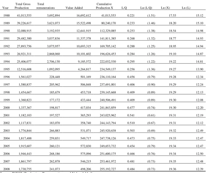
Table 8 Data Processing (Linear Model) Sub-Sector: Wood
Wood products including furniture (Thousands of USD Dollars at 2005 constant prices)
Year
Total Gross Production
Total
remunerations Value Added
Cumulative Production X L/Q Ln (L/Q) Ln (X) Ln (L) 1988 41,013,553 3,692,894 16,692,612 41,013,553 0.221 (1.51) 17.53 15.12 1989 39,226,617 3,621,073 15,522,498 80,240,170 0.233 (1.46) 18.20 15.10 1990 32,088,915 3,192,935 12,641,915 112,329,085 0.253 (1.38) 18.54 14.98 1991 29,482,300 3,037,836 11,337,378 141,811,385 0.268 (1.32) 18.77 14.93 1992 27,893,756 3,075,957 10,693,315 169,705,142 0.288 (1.25) 18.95 14.94 1993 26,921,311 2,868,060 10,101,602 196,626,453 0.284 (1.26) 19.10 14.87 1994 25,406,077 2,706,130 9,185,572 222,032,530 0.295 (1.22) 19.22 14.81 1995 12,516,608 1,092,095 4,264,817 234,549,137 0.256 (1.36) 19.27 13.90 1996 1,561,027 228,448 501,169 236,110,164 0.456 (0.79) 19.28 12.34 1997 1,580,837 205,962 506,848 237,691,001 0.406 (0.90) 19.29 12.24 1998 1,454,667 185,679 453,718 239,145,668 0.409 (0.89) 19.29 12.13 1999 1,360,823 177,172 433,444 240,506,491 0.409 (0.89) 19.30 12.08 2000 1,337,367 198,817 417,034 241,843,859 0.477 (0.74) 19.30 12.20 2001 1,182,103 197,527 365,293 243,025,962 0.541 (0.61) 19.31 12.19 2002 1,117,831 183,070 358,740 244,143,794 0.510 (0.67) 19.31 12.12 2003 1,776,844 266,883 531,071 245,920,638 0.503 (0.69) 19.32 12.49 2004 1,817,488 259,831 549,717 247,738,126 0.473 (0.75) 19.33 12.47 2005 1,915,607 260,121 572,830 249,653,732 0.454 (0.79) 19.34 12.47 2006 1,946,443 268,186 575,096 251,600,175 0.466 (0.76) 19.34 12.50 2007 1,861,797 262,878 546,215 253,461,972 0.481 (0.73) 19.35 12.48 2008 1,730,755 241,073 498,206 255,192,727 0.484 (0.73) 19.36 12.39
Source: INEGI (Production, Remunerations and Value Added)
Table 9 Linear Model Regression Results and Progress Ratio Value
Manufacturing Industry R2 F σ1 σ2 σ3 d Food 0.11 1.1 -4.64 0.09 0.08 1.061 Textile 0.51 9.24 -3.15 0.13 -0.02 1.096 Wood 0.89 70.73 -0.66 0.12 -0.19 1.083 Paper 0.81 37.68 -7.97 0.19 0.21 1.144 Chemicals 0.40 5.88 -7.79 0.10 0.29 1.068 Non-Metallic 0.81 38.70 -6.25 0.08 0.21 1.060 Basic Metals 0.60 13.74 -10.31 0.18 0.35 1.136 Machinery 0.95 166.98 -8.63 0.09 0.34 1.064 Others 0.86 53.85 -3.80 0.19 -0.06 1.142
27
Table 10 Progress Ratio Estimates by Sub-Sector (1988-2008)
Sub-Sector Progress Ratio Rank
Non Metallic 1.060 1 Food 1.061 2 Machinery 1.064 3 Chemicals 1.068 4 Wood 1.083 5 Textile 1.096 6 Basic Metals 1.136 7 Others 1.142 8 Paper 1.144 9
Total Mexican Manufacturing Industry 1.061
b) The Cubic Model Computation
As in the previous model, in this cubic model:
ln(L/Q) t= σ1 + BlnXt + C(lnXt)2 + D(lnXt)3 + σ2 lnLt
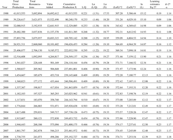
Total remunerations (L), value added (Q), and cumulative production (X) were used, and natural logarithm was applied following the model structure as detailed in Table 11 (For the rest of the sub-sectors, please referrer to appendix E).
The data was processed [Ln (L/Q), Ln (X), (LnX)2 , (LnX)3 and Ln (L)] in a regression
analysis to obtain the coefficients (σ1, B, C, D and σ2) which values are summarized in Table
12, and these coefficients were afterward used to estimate the learning elasticites according to
the above described formula α = - [B+ 2C lnXt+ 3D lnXt2].
The learning level (progress ratio) indices were calculated for every single sub-sector in the Mexican manufacturing industry as shown in Table 13.