What circular sector is to be cut out of a circle
so that the remaining surface maximizes the volume
of a symmetric upright cone with the same lateral surface?
Geogebra vs. Mathematica
Haiduke SarafianThe Pennsylvania State University University College
has2@psu.edu
Abstract
The main trust of this invcstigation is to apply Geogcbra and Mathematica to calculate the central angle of a circular sector that is to bc cut out of a circle of a given radius so that the remaining surface area maximizes the volume of a circular symmetric upright cone with the same lateral surface area. Solving the proposed problem on two different parallel tracks applying these Computer Algebra Systems reveals the pros and cons of these two pop‐ ular CASs. Utilizing the dynamic geometry of the former and its embedded CAS is compared to the sophisticated algebraic manipulation power of the latter. The investigation utilizes two and three dimensional visualization animations making the investigation comprehensive.
1 Motivation and Goals
Within the last decade Computer Algebra Systems especially Mathematica[ ] [ ] [ ] and Geogebra[ ] have deeply influenced structuring undergraduate and graduate mathemat‐ ics, science and engineering curriculums across the globe. Applying their superb two and three‐dimensional graphics adds new useful features to the analysis of the challeng‐ ing classic geometry problems opening fresh avenues exploring new challenging issues. In addition to thcir graphics thcsc software include symbolic manipulators capable of performing symbolic calculations. The author is an avid user of Mathematica and a recent user of the Geogebra. The main objective of this article is to compare their pros and cons analyzing a common geometry problem.
This note is composed of three sections and one appendix. In addition to Motivation and Goals in Sect 2 we describe the problem on hand and include its detailed solution. The appendix embodies Mathematica and Geogebra codes and their associated output. Sect 3 is the conclusion and closing remarks.
2
The problem and its solution
As is explained in the abstract the problem at hand is to calculate the central angle of a circular sector that is to be cut out of a circle of a given radius so that the remaining surface area maximizes the volume of a circular symmetric upright conc with the same
lateral surface arca.’\grave{3}
Figure 1 shows a disk with a cutout scctor. For the sake of simplicity the radius of the disk is set to unit. The area of the sector with the central angle is shown with the colorless wedge.
1 P1
-1 0
Figure 1. A unit disk with a cut out circular sector.
Area of the sector is
a=\displaystyle \frac{1}{2}R^{2} $\theta$
. For $\theta$=2 $\tau$\downarrow this yields the expected a= $\pi$ R^{2}.Extracting the surface area agives
\displaystyle \triangle A= $\pi$ R^{2}-a= $\pi$ R^{2}(1-\frac{ $\theta$}{2 $\pi$})
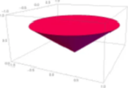
Utilizing this area wc form an upright conc with a circular base radius of r, hcight h
and side lengthl=R, respectively, shown in Figure 2.
11
11
Lateral area of the cone is
S= $\pi$ r\displaystyle \ell\equiv $\pi$ rR=\triangle A= $\pi$ R^{2}(1-\frac{ $\theta$}{2 $\pi$})
Simplifying yields r =
R(1-\displaystyle \frac{ $\theta$}{2 $\pi$})
, i.e. r =r( $\theta$). Volume of the cone is V =
\displaystyle \frac{1}{3}( $\pi$ r( $\theta$))^{2}h
, whereh=\sqrt{R^{2}-r( $\theta$)^{2}}
. Substituting for r( $\theta$) and simplifving givesV= (\displaystyle \frac{1}{6}R^{3}) (1-\frac{ $\theta$}{2 $\pi$})^{2}\sqrt{ $\theta$(4 $\pi$- $\theta$)}
In other words
V( $\theta$)= (1-\displaystyle \frac{ $\theta$}{2 $\pi$})^{2}\sqrt{ $\theta$(4 $\pi$- $\theta$)}
(1) Having this final result at hand it is a trivial task to find the angle maximizing the volumc. Howcver, as pointed out in thc abstract and the first Section, thc challenge is utilizing two and three‐dimensional graphics of Mathcmatica and Geogebra animating the process. In short first we claim the angle maximizing the volume is 66.060. Thiscomes about by solving V'( $\theta$) = 0 where V( $\theta$) is given by (1). Mathematica code
yielding this result follows. \mathrm{V}[$\theta$_{-}] :=
(1-\displaystyle \frac{ $\theta$}{2 $\pi$})^{2}\sqrt{ $\theta$(4 $\pi$- $\theta$)}
It is a helpful procedure to plot the function that we intend differentiating; this gives an objective view of the value of the variable optimizing the function.
Plot(V
[ $\theta$], \{ $\theta$, 0,2 $\pi$\}, GridLines
\rightarrowAutomatic, AxesLabel
\rightarrow\{\cdot $\theta$(rad)'',V(m3)})
-*
$\alpha$
\mathrm{d}V=D[V[ $\theta$], \{ $\theta$, 1\}] //Simplify
\displaystyle \frac{(2 $\pi$- $\theta$)(4$\pi$^{2}-12 $\pi \theta$+3$\theta$^{2})}{4$\pi$^{2}\sqrt{ $\theta$(4 $\pi$- $\theta$)}}
\mathcal{S}olV=Solve[dV==0, $\theta$]
\displaystyle \frac{180}{ $\pi$} $\theta$/
. solV3
Appendix
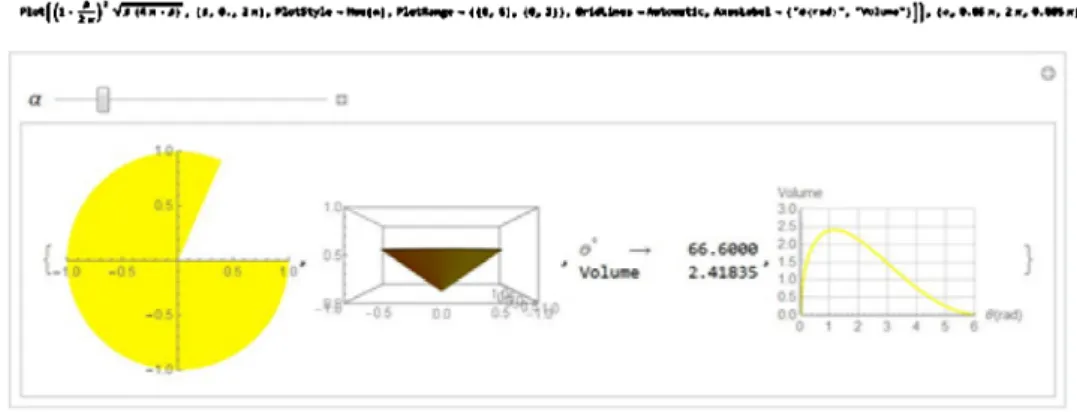
The main objective of this note is to compare graphics applications of Mathematica vs. Geogebra. Here we provide a version of the Mathematica code capable of animating thc entire proccss. Thc codc is dcscriptive; it embodies easy to follow commands. Commands are optimizcd producing thc nceded output. For instance the version of the code given in Figure 3 contains Manipulate as the main animation command. It follows by the Graphics Disk command. The combination of the last two sequential commands put the appearance of the disk in motion widening the central colorless area accordingly. The Cone command displays the cone and the Manipulate command put its evolution in motion. This is followed by displaying a table of the value of the angle and its corresponding conic volume. The code ends with a plot of the volume of the cone vs. angle. The author believes an expert Mathematica user would appreciate the
efficiency of the given four lines compact code producing the needed numeric, 2\mathrm{D} and
3\mathrm{D}graphics information.
-\mathrm{A}\cdot|\{\cdot \mathrm{r}:\mathrm{s}.(\mathrm{I}- $\sigma$], \mathrm{P}t $\vartheta$[1_{\bullet} $\eta$, l, a_{\bullet}3\mathrm{n}]]], iq\mathrm{p}\sim \mathfrak{n}\mathrm{w}, \prime 1\infty u \sim'' - l 1\}. \{-\mathrm{t}, 1))\downarrow,
\mathrm{W}\infty||-[\cdot|\cdot\wedgeÍ{l.l..\displaystyle \frac{1}{*}\frac{1\cdot-\cdot]}{}.|\mathrm{e}_{l}\mathrm{e}..|1,(\cdot\cdot\}1-\overline{*}..|}\bullet u.\rightarrow\mapsto_{l}\mathrm{P}\mathrm{W}t\leftrightarrow\rightarrow \mathrm{I} \mathrm{L}\}l. \leftarrow \mathrm{Z}_{\bullet}1/\mathrm{r}\mathrm{n}.1/\mathrm{f},--\bullet \mathrm{q}4-l_{\bullet} $\eta$|.
1\displaystyle \sim\dashv[-|_{\overline{l}}^{-}. .i \{t, \bullet $\iota$|, (-||$\iota$_{\overline{\mathrm{i}^{-}-}}-]'\frac{ $\sigma \alpha$_{---}}{\mathrm{t}\mathrm{I}}. $\iota \iota$, t\mathrm{J}]\}\}, \mathrm{r}\cdot \mathrm{I} \rightarrow[|..\cdot \neg.\prime\neg 4\mathrm{t}-\cdot|||,
r\displaystyle \mathrm{M}|(1\cdot\frac{}{2-}|^{1}\frac{l}{}(.-\cdot l|. \mathrm{t}\cdot, 0..\mathrm{l}\mathrm{n}\}, 4 $\iota$ \mathrm{v}4\neg\prime \mathrm{W}(\mathrm{Q}|, \mathrm{K}\leftrightarrow\neg 11\mathrm{C},l1\cdot 1_{l}1\}], .u\mathrm{D}l-\mathrm{i}\mathrm{W}\mathrm{b}\mathrm{g}\mathrm{P}\mathrm{t}\mathrm{S};, hrrl\neg( \cdot\{\bullet\cdot t). i\mapsto]||,\downarrow' lbr 1, arli.\leftrightarrow \mathrm{N})|
a \square \mathrm{Q}
.\mathrm{A}
0^{\cdot}
0
$\delta$. \rightarrow \mathrm{P}5.5\mathrm{K}
\bullet
iolwt
2.
\mathrm{e}\mathrm{i}s\supset 5
}
\mathrm{r}_{1}
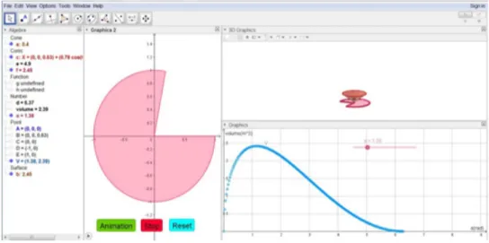
Figure 3. Output of the Mathematica code embodying all the needed information. Figure 4 is a screen‐shot of the Geogebra code and its output. The code embodies a different style of commands vs. Mathematica producing the needed information. The
screen‐shot is composed of one algebra screen on the left, two 2\mathrm{D} Graphics screens
and one 3\mathrm{D} Graphics screen. The inserted slider in the bottom right graphics screen
animates the plot. The colored animation buttons at the bottom of the Graphics 2 put the entire output to dynamic mode.
Figure 4. Screen shot of the Geogebra.
4 Conclusions
By way of example utilizing two different popular Computer Algebra Systems, Math‐ ematica and Geogebra the author compared their respective codes conducive to com‐ parable solutions. The author has been using Mathematica since its inception in 1985; he is a fresh user of Geobegra. As such he encountered a challenging but reward‐ ing learning curve. These two CASs are very powerful, they are fabricated assisting pursuing scientific goals. Their interfaces are totally different; they have different effec‐ tive and pleasant rewarding ‘(Havors.’; Based on the author’s experience for the future investigations he will adopt both.
References
[1] GeoGebra is a Dynamic Mathematics Software (DMS). It can be used as Dy‐ namic Geometry Software (DGS) with basic features of Computer Algebra Systems (CAS).
[2] \mathrm{M}\mathrm{a}\mathrm{t}\mathrm{h}\mathrm{e}\mathrm{m}\mathrm{a}\mathrm{t}\mathrm{i}\mathrm{c}\mathrm{a}^{TM} is a Symbolic Computation Software, V11.0, Wolfram Research
Inc. 2015.
[3] Wolfram, S. (1996) MMathematica book, 3rd Edition, Cambridge University Press. [4] Sarafian, H. (2015) Mathematica Graphics Example Book For Beginners, Scientific