A Two-Period Model of Capital Investment under Ambiguity (Financial Modeling and Analysis)

(1)

A Two-Period Model of Capital Investment under

Ambiguity*

Motoh Tsujimura

Faculty ofCommerce, DoshishaUniversity

1 Introduction

Animportantfactorin economic decisionmaking is thetreatmentofuncertainty. Knight (1921)

defines two kinds of uncertainty: risk, under which the probability ofan outcome is uniquely

determined; and uncertainty, under which it is not. The latter is termed Knightianuncertainty

or deep uncertainty. In this paper, following Ellseberg (1961),

we

term Knightian uncertainty

ambiguity. For a survey of decision making under uncertainty, see, for example, Camerer and

Weber (1992), Etner et. al. (2012) and Guidolin and Rinaldi (2013).

We examine capital investment under ambiguity in a two-period setting. We extend the

model ofMiao (2004), who investigates optimal consumption under ambiguity in

a

two-period

setting. We analyze a production economy and derive optimal capital investment in a

general-equilibrium setting. Suppose that there are a large number of identical

consumers

and firms

in an economy. For analytical simplicity, the number of consumers is equal to that of firms,

and

consumers

own the firms. This enables us to consider a representativeconsumer and firm.

The representative

consumer

is risk

averse

and has

a

constant absolute risk aversion utility

function. Because there is ambiguity, the representative

consumer

considers

a

set of probability

distributions. Then, we formulate the utility function

as

the multiple-priors expected utility

of Gilboa and Schmeidler (1989). We formulate the central planner’s problem and derive the

optimal level of capital investment. Furthermore, we analyze the comparative static effects of

the$mo$del’sparameters. Wefindthat ambiguityaversion and riskaversion have different effects

on capital investment. The more ambiguity averse the central planner, the higher the capital

investment. Bycontrast, at alowlevel ofrisk aversion, themore riskaversethe centralplanner,

the lower the capital investment. Once risk aversion has reached a certain level, increased risk

aversion stimulates capitalinvestment.

The rest of the paper is organized as follows. In Section 2, we describe the setup of the

production economy and formulate the central planner’s problem. In Section 3, we solve the

central planner’s problem. In Section 4,

we

conduct

a

numerical analysis. Section 5 concludes

the paper.

2 The Model

We consider atwo-period productioneconomy. There are alarge number ofidentical

consumers

and firms. The number of

consumers

is equal to that of firms. The firms

are

owned by the

consumers and produce identical outputs. We consider a representative consumer and firm.

’This researchwassupportedin part byaGrant-in-Aidfor Scientific Research(No. 24510213) fromthe Japan

(2)

The representative

consumer

receives an endowment in each period $t(t=1,2)$

.

This

endowment isa random variable on $(\Omega, \mathcal{F}, \mathbb{P})$

.

Therepresentativefirmproducesoutput byusing

capital $K$. The firm’s production function _$f(k)$ isgiven _by:

$f(k)=Ak^{\alpha}$, (2.1)

where $A>0$ reflects the level of technology and $\alpha>0$ is the output elasticity of capital.

The

consumer

receives utility from consumption $C_{t}$ in each period. The utility function $u(c)$ is

assumed to be given by:

$u(c)=- \frac{1}{\theta}e^{-\theta c}$, (2.2)

where the coefficient $\theta>0$ is the degree of absolute risk aversion. The representative

con-sumer maximizes the utility $u$ from consumption subject tothe following intertemporal budget

constraint:

$C_{1}+K=Y_{1}$, _(2.3)

$C_{2}=Y_{2}+(1-\delta)K+f(K)$, (2.4)

where $\delta\in(0,1)$ is the depreciation rate of capital. Suppose that the representative consumer

does not uniquely determine the probability distribution of future endowments but instead

considers

a

set of probability distributions. Then,

we

formulate the representative consumer’s

utility function

as

themultiple-priors expected utilityof Gilboa and Schmeidler (1989):

$U(C_{1}, C_{2})=u(C_{1})+ \beta\min_{\mathbb{Q}\in \mathcal{P}}\mathbb{E}_{\mathbb{Q}}[u(C_{2})]$ , (2.5)

where$\beta\in(0,1)$ isa discount factor and $\mathcal{P}$ is aset ofpriorsover $(\Omega, \mathcal{F})$

.

Following Miao (2004)

and Kogan and Wang (2002), we define $\mathcal{P}$ as:

$\mathcal{P}(\mathbb{P}, \phi)=\{\mathbb{Q}\in \mathcal{M}(\Omega);\mathbb{E}_{\mathbb{Q}}[\ln(\frac{d\mathbb{Q}}{d\mathbb{P}})]\leq\phi^{2}\}$, (2.6)

where $\mathcal{M}(\Omega)$ is the set of probability measures on $\Omega,$ $d\mathbb{Q}/d\mathbb{P}$ is the Radon-Nikodym derivative

and $\mathbb{E}_{\mathbb{Q}}[\ln(d\mathbb{Q}/d\mathbb{P})]$ is the relative entropy

index.2

This specification is based

on

robust control

theory.3

The parameter $\phi>0$ representsambiguity aversion. The higher $\phi$, themore ambiguity

averse the representative consumer,

We assume that $\mathbb{P}$

is the probability measure of the normal distribution with mean $\mu$ and

variance$\sigma^{2}$

. All probability measuresin $\mathcal{P}(\mathbb{P}, \phi)$ have normaldistributions. $\mathbb{Q}$ is theprobability

measure

of the normal distributionwith

mean

$\mu-h$andvariance $\sigma^{2}$, where $h>0$represents

the

mean distortion chosen by the decision maker. Then, the relative entropy of $\mathbb{P}$ and $\mathbb{Q}$ is given

by:

$\mathbb{E}_{\mathbb{Q}}[\ln(\frac{d\mathbb{Q}}{d\mathbb{P}})]=\frac{h^{2}}{2\sigma^{2}}$

.

(2.7)

The derivation of (2.7) isin Appendix A.

2Thisis also termed theKullback-Leibler divergence.

(3)

The representative firm maximizes profits, given prices and technology. We formulate the

central planner’s problem as:

$\max U(C_{1}, C_{2})$, (2.8)

$\{C_{1},C_{2},K\}$

s.t. (2.3) and (2.4).

Rewriting the central planner’s problem yields:

$\max_{\{K\}}\{-\frac{1}{\theta}e^{-\theta(Y_{1}-K)}+\beta_{\mathbb{Q}}\min_{\in \mathcal{P}}\mathbb{E}_{\mathbb{Q}}[-\frac{1}{\theta}e^{-\theta[Y_{2}+(1-\delta)K+AK^{\alpha}]}(]\}\cdot$ (2.9)

In the nextsection, we solve problem (2.9) and derive the optimal level ofcapital investment.

3 Optimal Capital

Investment

In this section, we derive optimal capital investment. From (2.9), we obtain:

$- \theta Y_{1}+\theta K=\ln\beta[(1-\delta)+\alpha AK^{\alpha-1}]-\theta[(1-\delta)K+AK^{\alpha}]+\ln(\max \mathbb{E}_{\mathbb{Q}}[e^{-\theta Y_{2}}])$

.

(3.1)

From the relative entropy expression, (2.7), we obtain:

$\ln(\max \mathbb{E}_{\mathbb{Q}}[e^{-\theta Y_{2}}])=\ln(\max_{h}[e^{-\theta(\mu-h)+\theta^{2}\sigma^{2}/2}])$

(3.2)

$=-\theta(\mu-\sqrt{2}\sigma\phi)+\theta^{2}\sigma^{2}/2.$

Substituting (3.2) into (3. 1) yields:

$- \theta AK^{\alpha}+\ln\beta[(1-\delta)+\alpha AK^{\alpha-1}]-\theta(2-\delta)K+\theta[Y_{1}-(\mu-\sqrt{2}\sigma\phi)]+\frac{\theta^{2}\sigma^{2}}{2}=0$

.

(3.3)

The optimal level of capital investment $K^{*}$ is derived from (3.3). Optimal consumption $C_{1}^{*}$ is

$C_{1}^{*}=Y_{1}-K^{*}$

.

If the production function exhibits constant return to scale $(\alpha=1)$, we obtain theexplicit solution:

$K^{*}= \frac{y_{1}}{2-\delta+A}+\frac{\log\beta(1-\delta+A)}{\theta(2-\delta+A)}-\frac{\mu-\sqrt{2}\sigma\phi}{2-\delta+A}+\frac{\theta\sigma^{2}}{2(2-\delta+A)}$

.

(3.4)

Otherwise, it is impossible to obtainanexplicit formula for $K^{*}$. In thenext section, we

numer-ically derive optimal capital investment.

4 Numerical

Examples

In this section, we numerically calculate the optimal level ofcapital investment $K^{*}$ and

inves-tigate its response to parameter changes. The basic parameter values are

as

follows: $Y_{1}=10$;

$\delta=0.5;A=3;\alpha=0.75;\beta=0.95;\mu=5;\sigma=2;\theta=1;\phi=1$. Given these values, optimal

(4)

Figures 1-5illustrate the results of thecomparativestaticsanalysisforoptimalcapital

invest-ment $K^{*}$. Figure 1 shows that although optimal capital investment _$K^{*}$ is initially decreasing

in

the coefficient of absoluteriskaversion$\theta$, oncerisk aversionhas reacheda certain level _{$(\theta=0.621$}

in thebase case), $K^{*}$ increases in $\theta$

.

This result impliesthat acentral planner who is barely risk

averse

initially will cut capital investment once he or she becomes more risk averse. However,

once

a certain level of risk aversion has been reached, the central planner’s capital investment

increases with his or her risk aversion.

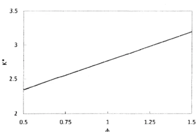
Figure 2 shows that optimal capital investment $K^{*}$ is increasingin thedegree of ambiguity

aversion $\phi$

.

Recall that a decision maker with a higher value of$\theta$is more averse to uncertainty.

Figure 2 implies thata central planner who is moreaverseto ambiguity invests more in capital.

Thisgenerates wealth in period 2.

Figure 3 shows that optimal capital investment is increasing in the volatility of endowments

$\sigma$. Such volatility leads a centralplanner toinvest more incapitalso that the riskof having less

wealth inperiod 2 is avoided.

Figure 4 shows that optimal capital investment is decreasing in the technology, represented

by the parameter $A$. Technological advancecauses less capital to be

needed by raising output.

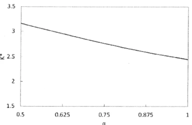
Figure5shows thatoptimal capitalinvestment is decreasing intheoutput elasticityofcapital

$\alpha$

.

This is because output increases in the output elasticity ofcapital.

$25$

2

0.$05$ 0.$3$ $0^{\ulcorner_{\backslash }\ulcorner}$ 0.$8$ $10_{:}^{\Gamma}$ $|..3$ $0$

(5)

$35$

1 $..-1$

($J$.5 075 ] 125 15 $\phi$

Figure 2: Comparative static effects of$\phi$ on optimal capital investment

$0 125 2_{i}\ulcorner) 375 5$

Figure

3:

Comparative static effects of $\sigma$

on

optimal capital investment

$0$ $25$ 5 $75$ 10

$A$

(6)

$3_{\lrcorner}^{}\backslash$ $\sim_{\sim_{\sim}}$ 3 $\sim_{\neg\sim}$ $\sim_{\sim\sim}$ $\sim_{=.\sim\sim}$ $*\cross 25$ $\sim_{\sim\sim\infty}$ $2\succ$ 15 $0^{r_{)}} (_{J^{\backslash }}7_{J}^{r} 0_{J}7^{\ulcorner} 0875 7$

Figure 5: Comparative static effects of$\alpha$ onoptimal capital investment

5 Conclusion

In thispaper,

we

analyzedcapitalinvestmentunderambiguity inatwo-period setting. We solved

the central planner’s problem and numerically derived the optimal level ofcapital investment.

Comparative statics analysis revealed that ambiguity aversion and risk aversion affect capital

investment differently.

There are several ways to extend this paper. Although Figure 4 shows that capital

invest-ment is affected by technological progress, we didnot consider uncertainty about technological

progress. Such uncertainty could be formulated by using the Poisson distribution. One could

also incorporate capital in addition to that used in production. For example, incases in which

production generates pollution, there is a need to invest in environmental capital that reduces

emissions. These important topics are left to future research.

References

Camerer, C. and M. Weber, Recent Developments in Modeling Preferences: Uncertainty and

Ambiguity, Journal

_of

Risk and Uncertainty, 5, 325-370, 1992.

Ellseberg, D., Risk, Ambiguity, and the Savage Axioms, Quarterly Journal

_of

Economics, 75,

643-669, 1961.

Etner, J., M. Jeleva and $J$.-M. Tallon, Decision Theory under Ambiguity, Journal

of

Economic

Surveys, 26, 234-270, 2012.

Gilboa, I. and D. Schmeidler, Maximin Expected Utility with Non-unique Priors, Journal

_of

Mathematical Economics, 18, 141-153, 1989.

Guidolin, M. and F. Rinaldi, Ambiguity inAsset Pricing and Portfolio Choice: A Reviewof the

Literature, Theory Decision, 74, 183-217, 2013.

Hansen, L.P. and T.J. Sargent, Robust Control and Model Uncertainty, American Economic

(7)

Knight, F.H., Risk, Uncertainty, and Profit, 1921.

Kogan, L. and T. Wang, A Simple Theory ofAsset Pricing underModel Uncertainty, Working

Paper, MITand University

_of

British Columbia, 2002.

Miao, J., A Note

on

Consumption and Savings under Knightian Uncertainty, Annals

_of

Eco-nomics and Finance, 5, 299-311, 2004.

Appendix

A.

Given the assumptions about the probability

measures

$\mathbb{P}$ and

$\mathbb{Q}$, we obtain

$\ln(\frac{d\mathbb{Q}}{d\mathbb{P}})=\ln(\mathbb{Q})-\ln(\mathbb{P})$

$= \ln(\frac{1}{\sqrt{2\pi}\sigma})-(\frac{(y-(\mu-h))^{2}}{2\sigma^{2}})-\ln(\frac{1}{\sqrt{2\pi}\sigma})+(\frac{(y-\mu)^{2}}{2\sigma^{2}})$ ($A$

.

1) $= \frac{-2h(y-\mu)-h^{2}}{2\sigma^{2}}.$

Then, relative entropy is

$\mathbb{E}_{\mathbb{Q}}[\ln(\frac{d\mathbb{Q}}{d\mathbb{P}})]=\int\ln(\frac{d\mathbb{Q}}{d\mathbb{P}})d\mathbb{Q}$ $= \frac{-2h(E_{\mathbb{Q}}[y]-\mu)-h^{2}}{2\sigma^{2}}$ ($A$.2) $= \frac{-2h(\mu-h-\mu)-h^{2}}{2\sigma^{2}}$ $=\underline{h^{2}}$ $2\sigma^{2}.$

Faculty of Commerce, Doshisha University

Kamigyo-ku, Kyoto, 602-8580 Japan

$E$-mail address: [email protected]