太陽光発電・蓄電池を用いた住宅規模での電力最適運用計画 (最適化手法の理論と応用の繋がり)

(1)

太陽光発電・蓄電池を用いた住宅規模での電力最適運用計画

出水宰，梅谷俊治，森田浩大阪大学大学院情報科学研究科情報数理学専攻大阪府吹田市山田丘1

Email: [email protected]

概要

近年，低炭素社会の実現に向けて，太陽光発電

($PV$ :Photovoltaic) _{などの再生可能エネルギーを} 導入した住宅規模でのエネルギーマネジメントが注目されている．昼間に $PV$_{で発電した電力を蓄電} 池に蓄えて夜間に使用することでの省エネルギー効果や，余剰電力を売電することでの省コストな電力利用が期待できる．しかし，$PV$の発電量や宅内消費電力量に伴う不確実性や，売電の価格体系及び電力の逆潮流に関する制約が将来的に変更される可能性などから，その運用には様々な検討がなされている．

本研究では，時空間ネットワーク

(TSN: Time-Space Network)

_{を用いて数理モデルを構築し，宅}

内規模での最適な電力運用計画を導出する．想定する環境は一般的な住宅内で $PV$ _{と蓄電池とが連携} し，$PV$_{の発電量や宅内消費電力に応じて電力運用を行うものとする．これらを TSN 上で表現し，各} ノード問の電カフローを変数として混合0-1整数計画問題に定式化する．これを解くことにより蓄電池の充放電タイミングや$PV$出力電力の配分などを決定し，宅内の電カコストを最小化する．また売電の価格体系や$PV$ の逆潮流方式の将来的な変動を考慮し，複数のマネジメントシナリオごとに最小の電カコストを導出し，運用方法の違いによるコストへの影響を解析する．数値実験では，実際の宅内消費電力量および$PV$_{発電量のデータを元にして季節ごとに}35_{日間のスケジュールを導出する．}

1 INTRODUCTION

In recent years, Smart Grid attracts attention as a new electric power system. The new system

controls the flow of electric power from the both sides of supply and demand and enablesusto use

efficiently electric power with high quality. In addition, it is expected that the renewable energy

such

as

photovoltaics ($PV$) leads to reduction ofgreenhouse gas. The Japanese govemment aims

at

a

spread of photovoltaics [1] and started feed-in tariff. However, the photovoltaics will change

due to

a

season, weather and time, so it has biginfluence

on

the other part ofthe electric power

system. Inorder to reduce thisinstability, it hasbeen proposedto introduce storagebatteries into

the grid[2, 3]. Then, it can stabilize the balance of electric power supply and demand by holding

surplus power generated in photovoltaics at daytime and storing electric power witha lowpriceat

night.

This paper considers an optimal electric power management using photovoltaics and battery

system. Assuming several management scenarios, we determine an optimal management plan for

each scenario and discuss their costs. In section 2, we define the electric power management

problem, and in section 3, we explain the mathematical model using a time-spacenetwork (TSN).

(2)

2 ELECTRIC

POWER

MANAGEMENT

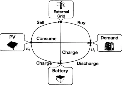
We consider electricpower managementin aresidentialbuildingusing photovoltaic and battery

system. Figure 1 shows the electric power network treated in this study. The demand ofelectric

powerin a residence differs at time, and the total supply from

an

extemal gird, $PV$and

a

battery

must satisfy the

demand

at every time. $PV$ generates electric energy _at _{each time, and it can}

distribute the energy to three demands, i.e., the extemal grid, the residential demand and the

battery.

In _{the current pricing system in Japan, the selling price is generally higher} _than _{the buying}

price. Therefore, everyone may consider to sell electricity by $PV$ asmuch as _{possible, and to buy}

necessary electricity in a residence. This is an incentive to introduce $PV$, however, _the _essential

purpose of introducing$PV$is localproduction for local_consumption, _not_to

_save

_electricity _cost_for

each

consumer.

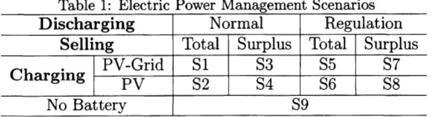
We

assume

_{two types of regulation in the operation of delivering} _electricity _from

$PV$back into the external grid.

1. Total amount type: The delivered power should be no more than the power generated by

$PV$

.

It is _possible _to _sell_{the total} _electric_energy_of_$PV$ _to _{the external grid.}

2. Surplus amount type : The electric

energy

of$PV$ is used preferentially for the residential

demand. The delivered power should be

no

more

than thesurplus power.

For the battery, we have to make the regulations in charging

resources

and dischargingtiming. If

there is no restriction on battery, that is, wecan charge battery from extemal grid

as

well as $PV,$

and discharge at any time, everyone may consider _{to charge the cheap electricity at night and to}

sell it during daytime by higher price, which is regardless the existence of$PV$

.

Here

we

_consider

two types ofregulation _{in discharging from the battery:}

1. Nomal type : Discharging from the battery is not forbidden. It is always possible to

dischargefrom the battery.

2. Regulation type: Discharging from the battery is forbiddenwhile$PV$ generateselectricity.

Thenit ispossible to dischargeonly during night or arainy day.

(3)

Moreover,

we

assume

two types of regulation in the

source

for charging the battery:

1. $PV$ and grid type: The battery can charge from $PV$ and the external gird.

2. $PV$ type: The batterycan charge fromonly $PV.$

There

are

several management scenarios by the combination of these constraints about $PV$ and

charging and discharging ofthe battery. Table 1 shows that electric power managementscenarios considered in this study. Here, the scenario Sl is the most flexible management. It is possible to

sell or to charge the electricity produced by $PV$, and also to charge the battery from grid. Since

Sl has no restriction on electric power flow, Sl gives us the lowest cost of electricity usage, ifwe

do not take into account ofthe cost of battery.

Comparing to Sl, we consider

some

scenarios. S3 isadded therestrictionthat theselling amount

ofelectricity does not exceed thesurplus. S5 is added the restriction that the discharging time is

limitedat night. S2 is added the restriction that the charging

resource

should be only $PV$

.

S4 is

thecurrent situationin Japan, where thebattery is notconnectedto

an

extemalgrid directly, and

prohibited to sell to and to buy from the grid. We note that we add scenario S9 which removed

the battery from the electricpower network inorder toverify the effect of abattery.

We also mention the unit price of electric power in Japan. When

we

buy electricity from the extemalsupplier inthe grid, theunit priceis a fixed rate, which varies depending

on

the timeand adayoftheweek. Onthe otherhand, when we sellelectricityback into thegridfrom $PV$, the unit

price is fixed and is set tomore expensive than buying price.

Table 1: ElectricPower Management Scenarios

3 MATHEMATICAL MODEL

We explain a formulation for the electric power management usingatime-space network (TSN)

model. TSN extends the usual network in the direction of a time-axis. Figure 2 shows a TSN

model for the electric power network in a residentialbuilding.

In this electric power network, wehave to determine the amount of flows between the nodes at

each time. Then, we formulate it as a mixed 0-1 integer programming problem ($0$-IMIP). In this

formulation, weuse abinaryvariablethat denotes the existence ofaflow. Itenablesus todescribe

constraints, such

as

the exclusion of charging and discharging operation of the battery, and the

prohibition of the inflow and the outflow via the external grid at the same time. Furthermore, by

using a continuous variable denotes the amount of a flow, we

can

describe the demand satisfied

constraint. Under these constraints we consider minimizingthe cost concerning electricpowerin

a

(4)

$PV$

Extemal

Gnd

Battery

Demand

$t-1 t t+1 t+2 t+3$

Time

Figure 2: Time-Space Network Model for the Electric Power Network

Input data

$p_{t}^{b}$ unit price

in buying electricity at time $t$

$p^{s}$ unit price in selling electricity

$C$ capacityof the battery

$g_{\max}$ maximum electric power chargedthe battery

hmax

maximumelectricpower discharged the battery

$\varphi$ decay rate from$AC$ to $DC$

$\psi$ decay rate from $DC$to$AC$

$T$ set of timeperiods for the management

$E_{t}$ electric power generated by_$PV$ at time $t$

$D_{t}$ demand in the residence at time$t$

$w_{0}$ initial rate ofelectricenergy onthebattery at time $0$

Decision variables

$x_{i,j,t}$ a binary variable denoting theexistence ofa flow from node $i$ to node_$j$ at time $t$

$y_{i,j,t}$ a continuousvariable denoting the amount ofa flow from node $i$ to node_$j$ at time $t$ $w_{t}$ rate ofelectric energy onthe battery at time $t$

Node symbols

$p$ node of$PV$

$c$ node of external grid

$s$ node of battery

$d$ node ofdemand

Formulation of mathematical model

Minimize

$\sum[(y_{c,d,t}+y_{c,s,t})p_{t}^{b}-y_{p,c,t}p^{s}]$ (1)

$t\in T$

subject to $y_{p,d,t}+y_{c,d,t}+\psi y_{s,d,t}=D_{t}$ (2)

$y_{p,c,t}+y_{p,d,t}+y_{p,s,t}=E_{t}$ (3)

$Cw_{t}+\varphi(y_{p,s,t}+y_{c,s,t})\leq C$ (4) $Cw_{t}-y_{s,d,t}\geq 0$ (5)

(5)

$\varphi(y_{p,s,t}+y_{c,s,t})\leq g_{\max}$ (6) $\{$ $x_{p,c,t}+x_{c,d,t}\leq 1$, (7) $\{$ $x_{p,s,t}+x_{s,d,t}\leq 1$, (8) $x_{p,c,t}+x_{c,s,t}\leq 1$ $x_{c,s,t}+x_{s,d,t}\leq 1$ $\varphi(y_{p,s,t}+y_{c,s,t})-y_{s,d,t}=C(w_{t+1}-w_{t})$ (9) $\{$

$\{\begin{array}{ll}0\leq y_{s,d,t}\leq h_{\max}\cdot x_{s,d,t}, 0\leq y_{p,c,t}\leq E_{t}\cdot x_{p,c,t}, 0\leq y_{p,d,t}\leq E_{t}\cdot x_{p,d,t}, (11)0\leq y_{p,s,t}\leq E_{t}\cdot x_{p,s,t}, \end{array}$ $x_{s,d,t}\in\{0,1\},$

$x_{p,c,t}\in\{0,1\},$ $x_{p,d,t}\in\{0,1\},$$x_{p,s,t}\in\{0,1\}$, (10)

$x_{c,d,t}\in\{0,1\},$$x_{c,s,t}\in\{0,1\}$

$0\leq y_{c,d,t}\leq D_{t}\cdot x_{c,d,t},$

$0\leq y_{c,s,t}\leq\simeq_{\varphi}\underline{\max}.$$x_{c,s,t}$

$0\leq w_{t}\leq 1$ (12)

In this formulation, we consider all the constraints in $t\in T$

.

The objective function (1) is the

total price calculatedby the amounts ofelectricity bought and sold via the extemal grid. Eq.(2)

implies the residential demand should be satisfied, and eq.(3) is the distribution constraint about

electric power generated by$PV$

.

Eqs.(4) and (5) show the capacity constraints of the battery with

charging and discharging. Eq.(6) shows the limit of electric power in charging the battery. Eq.(7)

shows theexclusionconstraints of buying and selling electricity via the extemal grid. Eq.(8) shows

the exclusion constraints of charging and discharging operations of the battery. Eq.(9) shows

the conservation of

electric energy

of charging

or

discharging

the

battery. Eq.(10) defines binary variables for each electric flow. Eq.(ll) defines the ranges for each electric flow. Eq.(12) shows the range ofthe charging rate of the battery.

This isa mathematicalformulation forscenario Sl,whichisa basic model

on

this study and the

otherscenarios can be described by adding several constraints to this formulation. For example, in

thescenario S3 and S4 weadd the followingconstraint about the amount ofdelivered power from

$PV$back into the extemal grid.

$\{\begin{array}{ll}y_{p,c,t}=0, t\in T_{1}=\{t\in T|E_{t}-D_{t}\leq 0\}y_{p,c,t}\leq E_{t}-D_{t}, t\in T_{2}=\{t\in T|E_{t}-D_{t}>0\}\end{array}$ (13)

Eq.(13) shows therestriction on the dehveredpower considering the surplus of the electric power.

Moreover, in the scenario $S5-SS$ we _{add the following} _constraint _{about the existence of the flow}

between the batteryand the demand.

$x_{s,d,t}=0, t\in T_{3}=\{t\in T|E_{t}>0\}$ (14)

Eq.(14) shows the prohibition of discharging from the battery while $PV$ generating. Finaly, we

consider the constraint about the scenario S2, S4, S6 and SS.

$x_{c,s,t}=0, t\in T$ (15)

Eq.(15) shows the prohibition of charging the battery from the external grid. Then the battery is

(6)

4 CASE STUDY

We

assume

the management scenarios and evaluate each minimum cost. We note that the

uncertainty about the amount of demand $D_{t}$ andthat of $PV$output $E_{t}$ is not consideredfrom the

viewpoint of compering the minimumcosts amongall the considered scenarios.

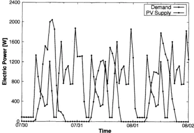
We get these data $D_{t}$ and $E_{t}$ from a real residential building for three different seasons, i.e.,

summer, winterand mid-term. Figure3shows changesfor every

one

hour in the demand of electric

energy and the supply by$PV$ at

summer.

Figure 3: Changes in Demandof Electric Power and Supply by $PV$

The management planning period of each season is 35 days. In each season, the unit price of

buying electricity from the external grid is fixed with time and a dayof the week. Table 2 shows

the unit price of buying electricity.

Table 2: Unit Price ofBuying Electricity

We have changedthe unit price of selling electricitybetween$0$and

45

$[yen/kWh]$ tosee how each

management scenario works and its minimum cost. We have used ILOG CPLEX 12.4 for solving

the$0$-IMIP.

We also note the other parameters about the management. The capacity of battery $C$ is 6

$[kWh]$, _{and the} _maximum _{electric power of both charging and discharging the battery,} _{$g_{\max}$} _and

$h_{\max}$, is 3 $[kW]$, respectively. Incharging and _{discharging the battery,} _{electric power}_is _decreased

because ofthe conversion between $AC$ and $DC$

.

The decay rate $\varphi$ from$AC$ to $DC$ is 0.9 and vice

versa.

Figures 4 and 5 show the comparison of the minimum cost over 35 days among the

seven

(7)

Figure4: Comparison ofthe Minimum Cost

over 35Daysamong 9Management

Scenarios

in Summer

Figure 5: Comparison of the MinimumCost

over 35Daysamong 9Management

Scenarios in Winter

From these figures,

we

obtainedthe following fourfindings:

1. The total cost decreasesgreatly by introducingabattery in

case

ofalowunit priceof selling electricity.

2. There is few effect ofbattery

as

the unit pricegoesup,when the

source

ofcharging

a

battery

is only $PV$such

as

S2, S4, S6 and SS.

3. Ifthereisno restrictionsuch asSl, the reduction of total costis remarkablein caseofahigh

unit price of selling electricity.

4. Comparingsummerand winter, thecharacteristicsbetween scenarios is almost samein spite

that the total cost has shifted.

In the next experimentation,

we

analyze the cost reduction effect of the management factors by using the analysisofvariance (ANOVA). There

are 4

factors, that is selhng, charging, discharging

and season, and they have each level

as

the table 3shown.

Table 3: Management Factors and Their Levels

Here, we

assume

season’s factor

as

an uncontrollable factor. Then we analyze the effect ofthe

other 3 factors and their interactions byremovingthis factor. Inthisexperiment, theunit priceof

sellingis fixed at 42 yen per $kWh$ andits price issame tocurrent Japan.

Figure6showthe resultofANOVA. Forthe factorial effect, there isasignificant difference in all

the factor. Especially, the factor of charging, that is factor $C$, shows the most significant effect of

the three factors. Between$PV$-Grid type and $PV$type, thereisacost differenceof 2,000 yen. Next,

for the interactioneffect, there is also asignificant difference in all. Especially, the interaction of Discharging and Selhng, that is Interaction $A*B$, is the most influential effect. At the level A2,

(8)

Factorial Effect of A Factorial Effectof$B$ FactorialEffectof$C$ $\overline{\underline{e\omega\wedge}}$ $\overline{\underline{\Phi=\succ}}$ $\overline{O\omega Q}$ $\mathring{0}{\}$ $\frac{\in}{\in}$ $\in E\ni$ $\overline{e}$ $\overline{\epsilon}$ $\dot{\overline{\Xi}}$ $\dot{\overline{\Xi}}$ Al A2 Bl B2 Cl C2

InteractionEffect of$A^{*}B$ Interaction Effectof$A^{\star}C$ lnteractionEffectof$B^{*}C$

$\overline{\underline{\Phi=>\backslash }}$

$\overline{\underline{c\omega}}$

誘

8 ぢ

$=\underline{\frac{\in 3}{\epsilon}\in}$ $=\underline{\frac{\in}{\epsilon}3\in}$

Al A2 Al A2 Bl B2

Figure 6: Effect of Factors and Interactions

5 CONCLUSION

In this study,wehave considered anoptimal electric power management ina residentialbuilding

using $PV$ and battery system. To get an _optimal _management _plan, we _{formulate the} _problem

as

$0$-IMIP through a TSN model. By solving it under several management scenarios, we show

the comparison of each minimum cost. Finaly, we analyze the cost reduction effect causedby the

management factors by using ANOVA.

REFERENCES

[1] Overview$of$”$PV$roadmap toward

2030”,

NewEnergy and Industrial_Development_Organization

(NEDO), Tokyo, (2004).

[2] B. Lu andM.Shahidehpour, Short-termscheduhngof bat-teryina grid-connected$PV$/Battery

system, IEEE transac- tionon power systems, vol. 20, no. 2, pp. 1053-1061, (2005).

[3] Y. Riffonneau, S. Bacha, F. Barmel and S. Ploix, Optimal power flow management for grid

connected$PV$systems with batteries, IEEE_{transaction on}_sustainable _energy, _{vol. 2,} _no. _{3, pp.}