Model Checking of Embedded Systems
Using RTCTL
Yajun Wu * and Satoshi Yamane †
* Graduate School of Natural Science and TechnologyKanazawa University, Kanazawa, Japan Email: [email protected]‐u.ac.jp
† Institute of Science and Engineering
Kanazawa University, Kanazawa, JapanEmail: [email protected]‐u.ac.jp
Abstract—For embedded systems, verifying both real‐ time properties and logical validity are important. In order to verify real‐time properties, we develop a simu‐ lator to propose model checking method. The simulator generates timed Kripke structure by dynamic program analysis. We implement the simulator to construct timed Kripke structure including the execution time. Also, we implement model checker in order to verify whether timed Kripke structure satisfies RTCTL formulas.
I. INTRODUCTION
In recent years, embedded systems have been widely used in autonomous car, medical equipment andIoT (Internet of Things). Verifying both real‐time proper‐ ties and logical validity are important for embedded
systems.
Recently software model checking [1] and program verification [2] have received widespread attention. S. Yamane and others have developed a verification system [3] for verifying embedded assembly programs. It generates Kripke structure by the simulator (dynamic program analysis) and verifies stack overflow by CTL (Computational Tree Logic) model checking.
In this paper, we will describe model checking using RTCTL (Real‐Time CTL) in order to verify whether timed Kripke structure satisfies real‐time properties. We develop the simulator to generate timed Kripke structure from assembly program. In our approach, we implement the simulator to construct timed Kripke
structure which includes the execution time. Also, we
implement model checker in order to verify whether timed Kripke structure satisfies real‐time properties. In general, as timed Kripke structure has infinite states, our approach is effective. In our study, to evaluate a proposed method, we conducted experiments with the implementation of the verification system.
II. RELATED WORKS
B. Schlich studied model checking by using static program analysis to verify assembly program, but real‐time properties are not verified. B. Schlich can verify the hardware dependency problem by using the assembly program [4].
E. A. Emerson and others proposed RTCTL, and also developed model checking algorithms for RTCTL [5]. But our semantics of RTCTL is quite different from E. A. Emerson’s semantics of RTCTL.
R. Alur and D. L. Dill studied timed automata
[6]. Timed automaton is an extension of a finite state
automaton, and is a model that describes the system by both discrete event and continuous time lapse according to state transitions. On the other hand, in this study, we develop discrete‐time timed Kripke structure for the execution time of assembly program. Our study is different from timed automata.
S. Yamane and others have developed a verification system. The simulator generates Kripke stmcture, and
model checker verifies CTL formulas. The simuıator
includes clock cycles while generating models, but real‐time properties and execution time are not taken into consideration. S. Yamane and others have de‐ veloped abstraction techniques by using DND (De‐ layed NonDeterminism) of the bit level. Our proposed method is quite different from [3] as follows: (1) Generating timed Kripke structure including execution time. (2) Using RTCTL formulas to verify real‐time properties. (3) Proposing RTCTL model checking al‐ gorithm after generating timed Kripke structure.
III. COMPUTATIONAL MODEL OF EMBEDDED ASSEMBLY PROGRAM
As a computational model, we define a timed Kripke structure which extends Kripke structure [7] by time function.
[Definition 3.1] (Timed Kripke structure) Timed Kripke structure is M=( S, S_{0}, R, L, TM).
(1) A finite set of states S. (2) A set of initial states S_{0}\subseteq S (3) A transition relation R\subseteq S\cross S
(4) A labeling function L:Sarrow 2^{AP}Lis a function
which assigns to each state a set of atomic propositions. AP is atomic proposition.
(5) A time function TM: Sarrow N TM is a function that assigns the execution time of each instruction to each state. Here Nis any natural number.
IV. RTCTL
For model checking of real‐time properties, we define Real‐Time temporal logic (RTCTL (Real‐Time CTL)). We use RTCTL developed by E. A. Emerson
[5].
[Definition 4.1] (Syntax of RTCTL) Syntax of RTCTL formulas as follows:
(1) Each atomic proposition AP is a RTCTL for‐ mula.
(2) If p, qare RTCTL formulas, similarly p\wedge qand \neg p are RTCTL formulas.
(3) If p, qare RTCTL formulas, similarly E(pUq), A(pUq) and EXp are RTCTL formulas.
(4) If p, qare RTCTL formulas and kis any natural number for execution time, similarly
E(pU^{\leq k}q)
andA(pU^{\leq k}q)
are RTCTL formulas.Some other RTCTL are defined as follows:
AF^{\leq k}q=A(
true U q)EF^{\leq k}q=E(
true Uq)
AG^{\leq k}p=\neg EF^{\leq k}\neg p
EG^{\leq k}p=\neg A\Gamma^{\leq k}\neg p
We propose the semantics of RTCTL as follows.
[Definition 4.2] (Semantics of RTCTL) In the se‐ mantics of RTCTL formuıas, other than
E(pU^{\leq k}q)
and
A(pU^{\leq k}q)
are the same as those of RTCTL by E.A. Emerson and others. Our semantics of
E(pU^{\leq k}q)
and
A(pU^{\leq k}q)
is quite different from E. A. Emerson’ssemantics [5]. In the semantics of
E(pU^{\leq k}q)
and A(pU^{\leq k}q)
is defined over timed Kripke structure M=(S,S_{0}, R, L, TM ) .
(1)
E(pU^{\leq k}q)
For a state sequence s_{0}, sı, . . ., s_{J}, . . ., s_{x}, . . . in
M, \exists i0\leq i, s_{i}\models qand
\sum_{\alpha=0}^{\iota}TM(s_{\alpha})\leq k
and \forall j0\leq j<i, s_{j}\models p.
(2)
A(pU^{\leq k}q)
For all state sequence s_{0}, s_{1}, . . ., s_{j}, . . ., s_{t}, . . . in
M, \exists i0\leq i, s_{i}\models qand
\sum_{\alpha=0}^{i}TM(s_{\alpha})\leq k
and \forall j0\leq j<i, s_{0}\models p.
V. VERIFICATION SYSTEM The verification system is shown in Fig. 1.
Fig. 1. Verification system
Next, the model checking algorithm of
E(pU^{\leq k}
q) is defined in Algorithm 1.
A(pU^{\leq k}q)
is almost the same asE(pU^{\leq k}q)
. We generate states for the verification target and output a timed Kripke structure by the simulator. Simultaneously, model checking is performed by inputting RTCTL formula and timed Kripke structure.We use |f| to denote the length of RTCTL formula
f(E(pU^{\leq k}q))
. The calculation of |f| is the same asthat of E. A. Emerson and others [5]. When |f'| is
the length of the CTL formula f'obtained from fby deleting time constraint, |f|=|f'|+cand cis the sum of
the lengths of the bit strings representing in binary the time constraint of f. Thus, we see that the complexity of executing the entire procedure
E(pU^{\leq k}q)
modelcheck is O(|f|(|S|+|R|)).
\frac{Algorithm1A1gorithmofMocelCheckE(pU^{\leq k}q)}{1S:=\{s|q\in L(s)\}}
2 for s\in S doL(s):=L(s)UE(pU^{\leq k}q)
3 N:=kH:=k ll initialize N and H
4 while S\neq\emptysetdo
5 choose s\in S
6 S:=S\backslash \{s\} // remove sfrom S
7 N :=H // update Nby H
8 for aıl tsuch that R(t, s)do
9 if
E(pU^{\leq H}q)\not\in L(t)
and N\geq 0and p\inL(t)then
10 H :=N‐ TM(s) // update H
11
L(t):=L(t)\cup\{E(pU^{\leq H}q)\}
12 S:=S\cup\{t\} // add tto S
13 else if N<0and S\neq\emptysetthen
14 choose y\in S// other path has not checked
15 choose
E(pU^{\leq H}q)
from L(y)16 choose H from
E(pU^{\leq H}q)
17 end if
18 end for all
19 if R(t, s)=\emptyset then //state s is the initial state
20 H:=N‐ TM(s)
21 if H<0and S\neq\emptysetthen
22 choose y\in S
23 choose
E(pU^{\leq H}q)
from L(y)24 choose H from
E(pU^{\leq H}q)
25 else if H\geq 0then
26 break 27 end if 28 end if 29 end if 30 end while 31 N:=H // update Nby H 32 if N\geq 0 33 return true
34 else return false
[Example 1] We will give an example in order to explain Algorithm 1. We specify verification property
by RTCTL as follows.
E(pU^{\leq 10}q)
We verify whether timed Kripke structure in Fig. 2 sataisfies
E(pU^{\leq 10}q)
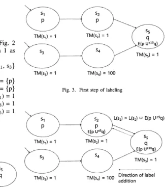
according to Algorithm 1 as follows. S= { s_{1}, s_{2}, s_{3}, S4, s_{5}} S_{0}=\{s_{1}, s_{3}\} R=\{ (s_{1}, s_{2}), (s_{2}, s_{5}), (s_{3}, s_{4}), (s_{4}, s_{5})\} L(s_{1})=\{p\} L(s_{2})=\{p\} L(s_{3})=\{\} L(s_{4})=\{p\} L(s_{5})=\{q\} TM(s_{1})=1 TM(s_{2})=1 TM(s_{3})=1 TM(s_{4})=100 TM(s_{5})=1Fig. 2. An example of timed Kripke structure
This formula is obviously satisfied since there is a path s_{1}arrow s_{2}arrow s_{5}.
To verify the RTCTL formula Algorithm 1 proceeds the following steps. Fig. 3, Fig. 4 and Fig. 5 give snapshots of Algorithm 1 in operation on the timed Kripke structure for the labeling function.
(1) In the first stage:
e Initially, S:=\{s_{5}\}(line 1) and L(s_{5}):=\{q, E(p
U^{\leq 10}q)\}
(line 2), as shown in Fig. 3. Then N:=10, H:=10(line 3).
0 Choose and remove s_{5} from S(line 4, 5, 6).
e Assign N :=H:=10(line 7).
0 There are two states s_{2} and s_{4} that satisfy R:= \{(s_{2}, s_{5}), (s_{4}, s_{5})\}(1ine8).
‐ Choose t=s_{2} first. Then assign H:= N‐
TM(s_{5}):=9 (line 10). Next add
E(pU^{\leq 9}q)
to L(s_{2})(line 11) as shown in Fig. 4, and add
s_{2}to S(line 12).
‐ Next, Choose t=s_{4} (line 9). But p\not\in L(s_{4}),
nothing to do here.
Fig. 3. First step of labeling
dUUI tlOrl
Fig. 4. Second step of labeling
(2) In the second stage:
e Now, S:=\{s_{2}\} (line 4). Similarly choose and
remove s_{2}and assign N :=H:=9 (line 7).
e There is one state s_{1}that satisfies R :=\{ (s_{1}, s_{2})\},
and choose it (line 8).
‐ Then assign H:=N-TM(s_{2}):=8(line 10).
Next add
E(pU^{\leq 8}q)
to L(s_{1}) (line 11) asshown in Fig. 5, and add s_{1} to S(line 12).
L(s_{1})=L(s_{1})\cup E(p\cup\leq 8q)
TM(s_{3})=1 TM(s_{4})=100 addition
Fig. 5. Third step of labeling
(4) Only in the final stage:
\bullet S:=\{s_{1}\} (line 4). Similarly choose and remove
s_{1}. Then assign N :=H :=8 (line 7).
e There is no state tthat satisfies R :=\{(t, s_{1})\}(line
8, line ı9).
\bullet Therefore, H\geq 0, then leave the loop, and updata
N=7(line 31).
\bullet Due to N\geq 0 . So the verification result becomes
true (line 33).
VI. EXPERIMENTS
We used LED program written by H8/3687 micro‐ controller [8][9]. The size of the program has 64 lines
of assembly code.
The execution time is obtained from the execution
state number of the assembly instruction. Since the operating frequency of H8/3687microcontroller is 20 MHz, the execution time per state is as follows.
1/20Mhz=0.05\mu s
Therefore, we assume the unit time of time con‐
straint k is 0.05\mu s.
The experiment was conducted on a laptop as fol‐ lows:
\bullet CPU : Intel(R) Core(TM) i7‐7700HQ processors
running at 2. 80GHz
e Memory : 16GB main memory
\bullet OS : windows 10
\bullet Simulator is written in a combination of Java and
Scala, and Model Checker is written in Scala as
follows.
\bullet Java 1.8.0_{-}121 , 15000 lines
\bullet Scala 2.11.8 , 6000 lines
\bullet Tools : JFlex [10], Jacc [11]
Program ı (LED program)lights up one LED by a sensor of the microcontroller outputs. The sensor can identify black and white. When the sensor of the microcontroller detects white, it outputs 1 and LED lights up, when it detects black, it outputs 0. Furthermore, we preset the sensor always detected white and it turns off immediately after the LED lights up. For example, Tota1\iota_{ed} times LED lights up by
Tota1\iota_{ed} times the sensor outputs. We specify timing constraints by RTCTL for this experiment as follows: RTCTL 1: EF^{\leq k}(Tota1\iota_{ed}=n)=E(true U (Tota1_{\iota}ed =n))
Tota1_{led}denotes the total number of lights up times. The nis the number of lights up times, indicated by
the value of the register RO in the state. The formula intuitively means that LED lights up Tota1_{\iota_{ed}} times happen at some state on some path from initial states within the timing constraint k. Besides we preset the specific LED light up number while timing constraint
kis limited within one millisecond (k=20000).
The experimental results are shown in Table I. The first column presents the total number of lights up times. The second column gives the number of states.
The third columm indicates the number of transition
relations. The fourth column presents the total time of simulator and model checking. The fifth column presents execution time of assembly program for some
path satisfies Tota1_{led} times lights up LED or the execution time of assembly program for a certain path is only not satisfied time constraint. The last columm shows the result which shows satisfiability of RTCTL formula. Execution time is obtained from the total execution time of executed states. The execution time of each state is an execution time of assembly instruction executed in each state.
TABLE I
THE RESULTS OF VERIFYING PROGRAM 1
n states rela ions ve ification execution result
\frac{time(s)time(ms)}{103703694.70.0507true}
50 1490 1489 23.3 0.2207 true
100 2890 2889 48.4 0.4332 true
200 5690 5689 115.0 0.8582 true
233 6614 6613 1_{l}18_{l}5 0_{:}998.5. true
30\ddot{0} 849Ô 84\dot{8}9 149.9 i\cdot.\cdot\dot{2}832 f^{r}alse
The experimental results showed the effectiveness of the proposed approach. We implement model checker in order to verify whether timed Kripke structure satisfies RTCTL formulas. These resulting data show that it can be verified whether or not lights up Tota1_{\iota_{ed}} times within the time constraint k. Moreover, as a result, we showed that the maximum number of LED
lights up within the time constraint k. As shown in
Table I, if nincreases, the number of states and the
number of transition relations polynomially increases.
Therefore, the verification time and execution time
polynomially increases. Further, when nbecomes 234
or more, the verification result becomes false.
VII. CONCLUSION
In this paper, we have developed a verification system. Model checker after generating timed Kripke structure by using RTCTL formula verifies whether timed Kripke structure satisfies real‐time properties.
In the case of RTCTL model checking after gener‐ ating timed Kripke structure, when the timed Kripke structure satisfies E(pUq) and does not satisfy time constraint k, we can figure out the execution time of that path by calculation. By doing so, when we repeat the experiment, we can know the time constraint is nearly satisfied with that path.
As future work, we will develop model checking of embedded systems using counterexample‐guided ab‐ straction refinement (CEGAR). And we will compare with model checking while after generating all states. Beside this, we want to detect other properties in embedded systems.
VIII. ACKNOWLEDGEMENTS
This work was supported by the Research Institute for Mathematical Sciences, a Joint Usage/Research Center located in Kyoto University.
REFERENCES
[1] Ranjit Jhana, Rupak Majumdar, ”Software modeı checking ACM Computing Surveys (CSUR) 41 (4), 2009: 21. [2] Leonardo de Moura, Nikolaj Bjorner, “Z3: An Ecient SMT
Solver,’‘ LNCS 4963, pp. 337‐340, 2008.
[3] S. Yamane, R. Konoshita, T. Kato, ’‘Model checking of embed‐ ded assembly program based on simulation IEICE Trans. In‐ formation and systems, Vol.E100‐D, No.8, pp1819‐1826, 2017. [4] Schlich, B, “’Model Checking of Software for Microcontrollers
ACM Transactions on Embedded Computing Systems 9 (4),
20ı0: 36
[5] E. A. Emerson, A. K. Mok, A. P. Sistla, J. Srinivasan, ”Quanti‐
tative Temporal Reasoning Real‐Time Systems 4 (4) pp. 331‐
352, 1992.
[6] R. Alur, D. L. Dill: “A theory of timed automata,’‘ TCS, ı26(2), pp. 183‐235, 1994.
[7] Edmund M. Clarke Jr., Orna Grumberg, Doron Peled, “Model Checking MIT Press, 1999.
[8] Corporation, R. E. : Renesas Electronics, Renesas Electronics Corporation (online), http://japan.renesas.com/
[9] nuvo WHEEL: ZMP, http://www.zmp.co.jp/products/wheel
[10] Klein, G.: JFlex ‐ The Fast Scanner Generator for Java, CSE
UNSW (online) , available from (http://jflex. de/)
[11] Jones, M. P.: Jacc: just another compiler compiler for Java, Department of Computer Science and Engineering at the OGI School of Science & Engineering at OHSU (online) , avaiıable from (http://jfiex.de/)