The Great East Japan Earthquake and its Short-run Effects
on Household Purchasing Behavior
Naohito Abe, Chiaki Moriguchi,
and
Noriko Inakura
March 31, 2012
Research Center for Price Dynamics
A Research Project Concerning Prices and Household Behaviors
Based on Micro Transaction Data
Working Paper Series No.2
Research Center for Price Dynamics
Institute of Economic Research, Hitotsubashi University
Naka 2-1, Kunitachi-city, Tokyo 186-8603, JAPAN
Tel/Fax: +81-42-580-9138
E-mail:
[email protected]
1
The Great East Japan Earthquake and its Short-run Effects
on Household Purchasing Behavior
*Naohito Abe Chiaki Moriguchi
Institute of Economic Research Institute of Economic Research Hitotsubashi University Hitotsubashi University
Noriko Inakura
Japan Center for Economic Research March 31, 2012
1. Introduction
The powerful earthquake that hit Japan on March 11, 2011, not only devastated towns and villages in the northeastern region, but also caused disrupted economic activities, affecting millions of firms and households far beyond the disaster-stricken areas. There has been a systematic effort to assess the direct damages caused by the Great East Japan Earthquake; however, few studies have attempted to empirically examine its economic consequences beyond the northeastern regions.
In particular, during the week immediately following March 11, the media widely reported severe shortages of essential goods—most notably, oil, batteries, flashlights, rice, bottled water, and toilet paper—in the areas that were not directly affected by the disaster. In Tokyo and other eastern cities, people encountered empty shelves, long waiting lines, and quantity restrictions (such as “one item per customer”) in major supermarkets. As the shortage of goods became a national concern, on March 14, the minister of consumer affairs made a public plea to refrain from “hoarding.” The shortages were primarily demand driven, specifically, a sudden increase in consumer demand as households faced greater future uncertainty with continuing aftershocks and unfolding nuclear power plant failures. At the same time, there were supply-side shocks to many commodities—most notably, milk, yogurt, fermented soybeans, and bottled water—due to
* The authors would like to thank Hidehiko Ichimura, Daiji Kawaguchi, Andrew Leicester, Makoto Saito, and seminar and conference participants at University of Tokyo, Osaka University, and Hitotsubashi University for their helpful comments and discussions. Financial support from JSPS Grants-in Aid for Young Scientists (S) 21673001 is gratefully acknowledged.
2
damaged production facilities, disrupted supply chains, and power shortages, resulting in large excess demand for the affected goods.
Even though anecdotal evidence abounds, we know very little about the actual effects of the 3/11 disaster on consumer behavior. To what extent did consumers increase their purchase after the earthquake? If the excess demand was resolved through some mechanisms of rationing, then did it create any discrepancy between those consumers who could stockpile goods and those who could not? In this paper, we take advantage of high-frequency micro panel data provided by Intage to investigate the short-run effects of the 3/11 earthquake on household purchasing patterns. To our knowledge, this is the first study to empirically examine the short-run effects of a large disaster on consumer behavior.
The main findings of the paper are as follows:
(1) In the eastern prefectures not directly affected by the disaster, household expenditure on storable foods rose sharply in the week following March 11. However, the spike in the expenditure was temporary.
(2) Despite the excess demand induced by the disaster, the food price index increased slowly and modestly. In other words, household expenditures in the eastern area increased, not owing to higher prices, but primarily owing to larger quantities purchased.
(3) We use a model of consumer purchase with inventory to investigate the effects of the disaster on stockpiling behavior. We find that the number of major tremors experienced by households had negative effects on the likelihood of making any purchase in the week following March 11 but positive effects on the amount of purchase in that week conditional on making a purchase. We also find that, compared to the average household, households with a young child had a lower likelihood of making any purchase in response to the disaster, while an increase in food expenditure in response to the disaster was smaller for households with a working wife. (4) Although we cannot distinguish households who intended not to purchase any foods from those who intended but could not, our results suggest that households with higher opportunity costs of shopping were more likely to be “rationed out” and could not purchase foods. In other words, the disaster and resulting shortages of essential goods might have increased the discrepancy between those households who were able to stockpile foods and those who could not.
The rest of the paper is structured as follows: in Section 2, we describe the Great East Japan Earthquake and show the geographical distribution of its seismic impact; in Section 3, we present the data; in Section 4, we examine the responses of commodity prices to the disaster; in
3
Section 5, after introducing an inventory model of consumer purchase, we provide empirical analyses of household purchasing behavior; and Section 6 concludes this paper.
2. The Geography of the Great East Japan Earthquake
A powerful earthquake hit the northeastern region of Japan on Friday, March 11, 2011, at 2:46 pm. According to a seismic intensity measure defined by the Japan Meteorological Agency, Miyagi, the prefecture closest to the epicenter, recorded the maximum intensity of 7 (equivalent to magnitude 9.0 on the Richter scale). It was the fourth largest earthquake in the world since 1900. In Fukushima, Ibaraki, and Tochigi, the recorded intensity was the second highest, higher than 6 on the Richter scale. The seismic intensity in Tokyo was higher than 5. Although Tokyo escaped direct damages, about 20% of the workers in central Tokyo could not return to their homes on the day of the earthquake owing to disrupted transportation services.
As the epicenter was 130 km from the seashore, within 40 minutes enormous tsunami followed the earthquake and devastated the Pacific coastal areas of the Iwate, Miyagi, and Fukushima prefectures. Because of the failures of the nuclear power plants in Fukushima and the resulting electric power shortages, the government announced (and partially implemented) scheduled rolling blackouts in the areas that were supplied electricity by the Tokyo Electric Power Company from March 14 to March 28.
After the huge earthquake on March 11, numerous large aftershocks hit the eastern part of Japan.
Figures 1-(a) to 1-(c) show the number of “major” tremors, defined by a tremor of seismic
intensity greater than 3, in two-week intervals in each prefecture.1 Note that, as we define Week 2 as the second week of January 2011 starting with Friday (i.e., Friday, January 7–Thursday, January 13), March 11 (Fri.) corresponds to the first day of Week 11.
Figure 1-(a) shows the number of major tremors in Weeks 8 and 9, representative weeks before
the 3/11 earthquake, indicating that only two prefectures experienced major tremors. The frequency skyrocketed in Weeks 11 and 12, and almost all prefectures in eastern Japan experienced more than 10 major tremors in these two weeks (see Figure 1-(b)). In Iwate, Miyagi, Fukushima, and Ibaraki, more than 20 major tremors were observed in Week 11 alone. By contrast, the western half of Japan experienced no tremors greater than intensity 3. As shown in Figure 1-(c), many eastern prefectures continued to experience major aftershocks in Weeks
1 The data on the frequency and intensity of tremors were obtained from the Japan Meteorological
4 13 and 14.
As shown above, the intensity and the frequency of the 3/11 earthquake and its aftershocks differed substantially across prefectures. In the subsequent analysis, we take advantage of the geographical heterogeneity of the major aftershocks. For the purpose of analysis, we define three areas, “Directly Affected Area,” “East,” and “West,” as shown in Figure 2. “Directly Affected Area” consists of four prefectures, Iwate, Miyagi, Fukushima, and Ibaraki, that received major damages from the earthquakes, tsunami, and nuclear power plant failures. In the following consumer behavior analysis, we exclude “Directly Affected Area” as consumers in this area were under extreme conditions. “East,” our treatment region, consists of seven prefectures that were not directly affected by the disaster, but nonetheless experienced at least one major tremor in Weeks 11 and 12 and were subject to rolling blackouts, including Tokyo, Kanagawa, Chiba, Yamanashi, Gunma, Saitama, and Shizuoka. “West,” our control region, consists of all prefectures that experienced no major tremor in Weeks 11 and 12, including Fukui, Toyama, Shiga, Mie, and all prefectures to the west of Mie, excluding Okinawa. Regression analysis using prefecture-level data below are performed with the data for all prefectures except “Directly Affected Area” and Okinawa.
3. Data
In this paper, we use two data sets, consumer panel data (hereafter SCI) and retail panel data (hereafter SRI) provided by Intage, a leading market research company in Japan, to support research on the impact of the 3/11 earthquake.
SCI contains the daily shopping information of approximately 12,000 households, randomly selected from all prefectures (except Okinawa) in Japan. The sample households are restricted to married couples. Using a barcode reader, households are asked to scan the barcode of every commodity they purchase, and scanned data are automatically transmitted to Intage’s datacenter. In SCI, for every commodity purchased, we can observe: (1) Japanese Article Number (JAN), a unique commodity identifier, (2) date of purchase, (3) price and quantity, and (4) store name from which the commodity was purchased. The data cover more than 10,000 commodities in 214 commodity categories comprising 146 categories of processed foods (e.g., rice, pasta, milk, sugar, condiments, and canned or frozen foods) and 68 categories of basic goods (e.g., toiletries, kitchen equipment, and cleaning tools).2 Fresh foods (e.g., meat, fish, and vegetables) without
2 Abe and Niizeki (2010) provide detailed comparisons between SCI and official consumption surveys
5
barcodes are excluded. We can also observe basic households characteristics, such as the ages of husband and wife, household income, education, household size and composition, and the prefecture of residence. The data is for the period from January 1 to May 31, 2011
SRI contains weekly transaction data from approximately 2,600 retail stores located in all prefectures in Japan. It covers multiple types of retail stores, including general merchandise stores, convenient stores, discount stores, drug stores, and individual stores. In SRI, for each store and for each commodity, we can observe (1) JAN, a unique commodity identifier, (2) week of transaction, (3) total quantity sold, (4) total sales, (5) store location, and (6) store type. In addition, we obtain more detailed commodity information for five categories (rice, cup noodles, natto, milk, yoghurt, and bottled water). The data corresponds to the period from the first week of January (Week 1) to the last week of May 2011 (Week 22). We drop Week 1 observations from our sample, as household expenditures deviate from normal patterns during the New Year holidays in Japan.
4. The Short-run Responses of Expenditures and Prices
To check whether consumers increased their purchases in response to the 3/11 earthquake, we first look at the movements of household expenditures using SCI daily data. In Figure 3, we plot the average household food expenditure (expressed in 1,000 yen) in “East” and “West,” as defined above, from January 8 to May 22. Throughout the sample period, in both East and West, we observe a spike in food expenditures on every weekend. In East, food expenditures fell sharply on March 11, then rose dramatically during three days after the earthquake, from March 12 (Sat.) to 14 (Mon.), and then declined to a level below the pre-disaster average during the rest of March. By contrast, in West, food expenditure patterns change little before and after March 11.
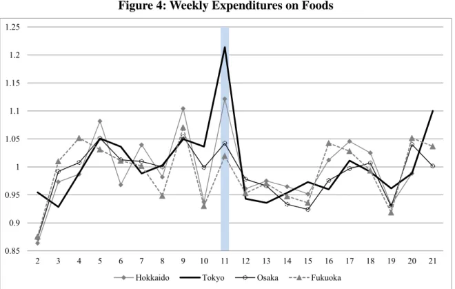
Next, in Figure 4, using SCI weekly data, we compare the movements of food expenditures in four major prefectures—Hokkaido, Tokyo, Osaka, and Fukuoka (see Appendix Figure 1 for their locations. For each prefecture, we normalize the average expenditure in the pre-disaster weeks (Weeks 2–10) to be unity. In Tokyo, the expenditure in Week 11 (March 11–17) increased by 22% compared to the pre-disaster average and then declined to a level lower than the pre-disaster level for many weeks. Although the expenditures in Hokkaido and Osaka exhibit similar patterns, their changes were modest in comparison to Tokyo. In Fukuoka, which is about 1,000 km away from the epicenter, the average expenditure did not respond to the earthquake. categories.
6
Although not shown in Figure 4, in the directly affected prefectures such as Iwate and Miyagi, household expenditures fell in Week 11 and declined further in Week 12, showing patterns that were different from the rest of Japan. It suggests that consumers in the directly stricken areas had difficulty in purchasing enough goods to maintain a pre-disaster level of consumption. Owing to a large decline in the number of sample households reporting the data after March 11 in these prefectures, it is difficult to examine their conditions in detail.
According to Figures 3 and 4, household expenditures surged immediately in response to the 3/11 disaster in the eastern prefectures outside the Directly Affected Area. However, this per se is not an evidence of “hoarding” behavior, since a surge in expenditures could result from higher prices. Therefore, it is important to investigate changes in commodity prices.3
When constructing a price index, we need to compute the rate of price change for each commodity. That is, for both base and comparison weeks, we need information on commodity prices. Unfortunately, the sample size of SCI was not large enough to compute category-level price index, as we encountered zero transactions for many commodities. Therefore, we used the SRI data to construct a price index at the category level.
Using the SRI weekly data, we computed the Fisher price index for foods in the four major prefectures, using Week 2 as the base week.4 As shown in Figure 5, in Tokyo, the food price
index increased by 1.4% in Week 11 when the average food expenditure rose by 21% according to Figure 4. The food price index in Tokyo increased by 5.0% by Week 13 and subsequently began to decline, but remained at a slightly higher level than the pre-disaster level during the rest of the sample period. In Hokkaido, the food price rose by 1.0% in Week 11, when the food expenditure rose by 12%. In Osaka and Fukuoka, there is no clear change in the food price levels. In other words, despite the presence of excess demand for a wide range of goods after the disaster, commodity prices responded only slowly and to a small extent.
More detailed analysis revealed that within-store commodity prices increased only by a maximum of 4–5% even for those commodity categories for which excess demand was large (e.g., cup noodles, milk, and bottled water).5 This indicates that retail stores tended not to raise
3 In a separate paper, we examine the effects of the 3/11 disaster on commodity prices in detail using SCI
and SRI data. See Abe, Moriguchi, and Inakura (2012) for more analysis.
4 We follow Ivancic et al. (2011) when constructing Fisher, Laspeyres, and Paasche price indexes. See
Appendix Figure 2 for the comparisons of the three indexes.
7
their commodity prices despite the sudden increase in demand, and chose rationing by queue or quantity restrictions to allocate scarce commodities to their customers. As many consumers shifted their demand to stores with higher prices6 or to similar but higher-priced commodities, category-level prices increased more than commodity-level prices for these categories with large excess demand.
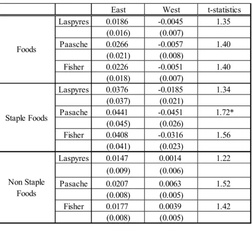
In Table 1, we compare the change in the food price index from Week 10 to Week 11 in “East” and “West” (For robustness, the results for Laspeyres, Paasche, and Fisher price indexes are shown). The weekly inflation rate in food price in East, measured by Laspyres price index, was 1.9%, while that in West was -0.5%. The two rates, however, are not significantly different in the statistical sense. When we categorize foods into “staple” foods (rice, bread, noodles, flour, and pancake mix) and “non-staple” foods (all the rest), the inflation rate of staple foods was significantly higher in East (4.4%) than in West (-4.5%) when measured in Paasche index. There was no significant difference in the inflation rates of non-staple foods. Although we observe a significant difference in some cases, overall, the rate of price increase in East was rather small and not much higher than that in West.
5. The Effects of the 3/11 Disaster on Household Expenditure Patterns 5.1 A Model of Consumer Purchase with Inventory
In the previous section, we observed that the responses of commodity prices to the 3/11 shocks were surprisingly modest. In other words, the surge in household expenditures in Week 11 observed in East was primarily due to an increase in the quantity purchased. To understand households’ short-run responses to the disaster better, we consider a dynamic model of consumer purchase with inventory, developed by Erdem et al. (2003) and Hendel and Nevo (2006a, b). In this model, a good is assumed to be storable and consumers decide the timing and the amount of purchase given a stochastic price process. For storable goods, because the time of consumption can differ from the time of purchase, the expenditures tend to concentrate during the period of low prices. A simulation by Erdem et al. (2003) using the data for ketchup shows that consumer expenditures surge during bargain sales and fall in subsequent periods. High frequency data, such as ours, are particularly useful in investigating consumers’ stockpiling behavior.
6 Many commodities are sold at different prices across stores. In general, convenience stores charge
8
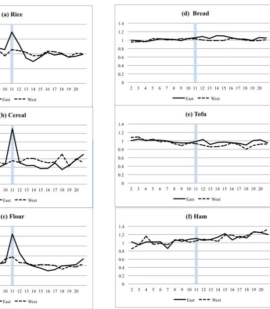
To see if such a model is applicable to our data, we first compare actual household expenditures on storable goods and non-storable goods. In Figures 6-(a) to 6-(f), we show the movements of expenditures on six food categories in East in contrast to West. As before, we normalize the average expenditure in Weeks 2–10 to be unity. Of the six categories, rice, cereal, and flour are storable, while bread, tofu, and ham are perishable. Compared to West, the household expenditures on storable foods in East show a clear spike in Week 11 and then a decline to a level lower than the pre-disaster average. This is consistent with the predictions of the inventory model of consumer purchase described above. For perishable foods, the household expenditures in East increased only slightly in Week 11.
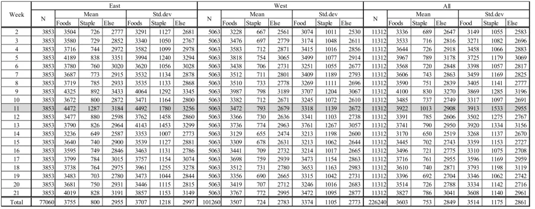
In the following analysis, rather than focusing on a specific commodity category and developing a nonlinear dynamic model, we analyze a composite good by aggregating commodity categories and conduct a reduced form analysis.7 To be concrete, we analyzed three composite goods, namely, all foods, staple foods (rice, bread, cereal, noodles, flour, pancake mix), and non-staple foods. Table 2 provides descriptive statistics of weekly expenditures on these goods from Week 2 to Week 21. Most notably, the average expenditure on staple foods in East rose by 61% from 800 yen to 1,287 yen in Week 11 (March 11–17). Not only the level, but also the variance of household expenditures on staple foods increased in Week 11, suggesting that the heterogeneity across households increased after the disaster (see Appendix Table 2).
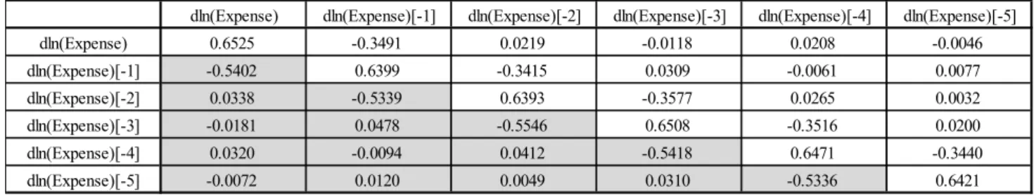
Table 3 provides the covariance structures of the weekly changes in the expenditures of foods,
staple foods, and non-staple foods. For all goods, the autocorrelation with its first lag is about -0.5, suggesting strong negative relationships between current and future expenditure growths. Note that, if expenditure follows a random walk, the first autocorrelation should be zero. The negative autocorrelations shown in Table 3 are similar to those obtained by Erdem et al. (2003) in their model. In the following analysis, we treat the three composite goods (foods, staple foods, and non-staple foods) as storable goods, and use a model of home inventory.
5.2 Estimating the Effects of the 3/11 Disaster on Stockpiling Behavior
Previous research on the determinants of optimal home inventory (Erdem et al., 2003; Hendel and Nevo, 2006a, b) has focused on the effects of uncertainty about future prices. In the case of the 3/11 disaster, however, we expect sudden and profound shifts in households’ perception of
7 Existing studies, such as Erdem et al. (2003) and Hendel and Nevo (2006b), focus on a few categories,
such as ketchup or detergent and estimate dynamic consumer choice using a nonlinear model. To implement this, however, we need information on the dynamic processes of multiple commodity prices and unobservable preference shocks.
9
future uncertainty after the disaster. In the days following March 11, it must be noted that: (1) numerous aftershocks were raising the fear of future major earthquake; (2) nuclear power plant accidents were still unfolding with consecutive hydrogen explosions on March 12, 14, and 15; (3) to prevent major electric power failures, the government released a daily schedule for rolling blackouts, creating much confusion; and (4) the shortages of essential goods were widely reported with a rumor of people engaging in “hoarding.” We assume that all of these factors influenced consumers’ subjective assessments over future uncertainty and led them to re-optimize the level of inventory to maintain a sufficient level of future consumption.8
First, we postulate that a household’s subjective assessment of future uncertainty increases with the number of major tremors experienced. If so, the households experiencing more tremors would raise their optimal inventory level to a greater extent and increase their expenditures accordingly. To test this hypothesis, we use prefecture-level variations in the weekly frequency of major tremors of intensity greater than 3 (presented in Appendix Table 1). It is important to emphasize that in the subsequent regression analyses, we drop observations after Week 11. As we have shown, many eastern prefectures continued to experience major aftershocks in Week 12 and beyond (see Figure 1-(c)), which in itself should further increase household expenditures in these prefectures. At the same time, however, there are strong negative autocorrelations in expenditure growths (see Table 3) indicating that those households that increased expenditures in Week 11 should reduce expenditures in Week 12. As a result, without knowing the level of home inventory in Week 11, we cannot identify the effects of major tremors in Week 12. As we drop the observations in Weeks 12–21 from the following analyses, we focus on the effects of the major tremors on the expenditure increase in Week 11.
As the base specification, we estimate the following equation regarding the change in weekly expenditure, , of household i in week t (t = 4, 5,…, 11):
E it t it E it E E it
c
Tremors
X
T
E
1 (1)where c is a constant, Tremorsit is the square root of the number of major tremors household i experienced in week t; Xit is a vector of household characteristics (household income, wife’s age and work status, household size and composition); and Tt is time effects captured by week
8 According to an internet survey conducted by Prof. Shigeo Tachiki of Doshisha University in April
2011 among 3,643 consumers (all residing outside the disaster-stricken areas) who increased the volume of purchase of some goods during the week following March 11, 48% replied that the reason for this behavior was “to prepare for power shortages and water supply disruptions” (multiple answers allowed), 32% said it was “to prepare for future disaster evacuation,” 31% said it was “to feel assured in fear of future disaster,” and 25% said that it was “to increase stockpiles for new disaster.” About 10% replied that they increased purchases because they felt anxious on hearing about other people hoarding.
it
E
10 dummies.
Next, we investigate the heterogeneity across households in purchasing behavior after the disaster. Recall that the price index did not increase much in Week 11. This suggests that temporary excess demand induced by the disaster was resolved mainly through quantity adjustments, most notably, “rationing by waiting” and “quantity restrictions.”9 Under these allocation mechanisms, we expect that households with lower opportunity costs of shopping can purchase a higher quantity of scarce commodities (by lining up or visiting many stores). In a recent study, Aguiar and Hurst (2007) show that the opportunity costs of shopping play a major role in optimal consumption decisions by using husband’s retirement status as a proxy for the opportunity costs. In our analysis, we focus on two variables: the presence of an infant and the wife’s work status. We postulate that households with at least one infant (child of age 0–3) have higher opportunity costs of shopping than those without. Similarly, we postulate that households with a wife working full-time have higher opportunity costs of shopping than those with a wife not working or working part-time.10
To further investigate household purchasing behavior, we introduce two additional variables: shopping frequency and shopping interval. Shopping frequency is the number of purchases a household makes in a week (see Appendix Table 3 for descriptive statistics). Because we observe only the date of purchase and the name of store from which the purchase was made, however, we compute shopping frequency assuming that a household makes purchases from the same store only once a day. Moreover, note that if a household visited a store but did not make any purchases (this may happen when goods are sold out), then it is not counted as shopping.
Shopping interval is measured in weeks and captures the number of weeks that passed since the last purchase (see Appendix Table 4 for descriptive statistics). If a household purchases food every week, the interval is one. However, for storable foods, especially rice and pasta, many households do not make purchases every week. In general, a longer shopping interval is associated with a higher likelihood of purchase in the current week. As such, it is important to control for shopping interval while analyzing the effects of the disaster on subsequent shopping behavior.
To investigate household heterogeneity in response to the disaster, we estimated the following equation:
9 For recent empirical analysis of rationing by queuing, see Batabyal and DeAngelo (2012).
10 According to the 2005 Census data, 50% of married women under the age of 35 in Japan do not have
11
,
4 3 2 1 E it t it E it it E i E i E E E itT
X
Tremors
Shopping
Fulltime
Infant
c
E
(2)
where Infanti and Fulltimei are dummy variables that indicate the presence of an infant and a wife working full-time in household i, respectively, and Shoppingi is the number of purchases (shopping trips) made by household i in week t. We interact each of these variables with the number of tremors experienced by household i.
Table 4 presents descriptive statistics of the variables used in the regressions. In our sample,
12.5% of households have an infant and 14.5% of households have a wife working full-time. The average household purchases foods 3.0 times per week, while the average shopping interval for foods is 1.36 weeks or 9.5 days (note that if all households make purchases every week, the interval would be 1.0). It is important to note that the standard deviations for both shopping frequency and shopping interval are large, indicating that there is great heterogeneity across households in their purchasing patterns.
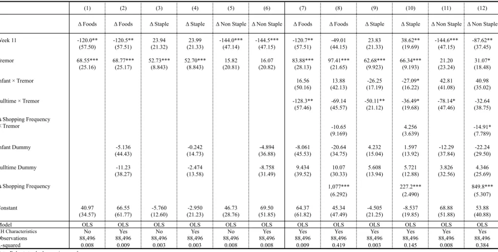
The estimation results for the three goods (all foods, staple foods, non-staple foods) are reported in Table 5. In almost all specifications, the number of major tremors has large, positive, and significant effects on the changes in expenditures. (The effects for non-staple foods are smaller and less significant than those for staple goods.) That is, households who experienced more major aftershocks in Week 11 stockpiled more food. On examining the effects of household characteristics in specification (10), the wife’s work status and the presence of an infant have little effect on the expenditures for staple goods in the pre-disaster weeks. The coefficients of the interaction terms, Infant×Tremors and Fulltime×Tremors, however, are large, negative and significant. It shows that, compared to the average household that increased the weekly expenditure on staple foods by 66 yen in response to major tremors, the households with a working wife and those with an infant increased their expenditures only by 30 yen and 39 yen, respectively. The coefficient of Fulltime×Tremors is smaller in specification (10) compared to specification (9), suggesting that the households with a working wife did not increase their expenditures on staple foods in Week 11 as much partly because they had lower frequency of shopping. The same is true for non-staple foods. For the households with an infant, by contrast, the results for staple foods and non-staple foods seem qualitatively different.
5.3 Considering the Extensive and Intensive Margins of Purchasing Behaviors
12
expenditures in Week 11 into extensive and intensive margins. Consider a household that usually purchases rice every other week. If the household purchased rice in Week 10, the next purchase would not occur in Week 11. If the 3/11 disaster suddenly raised the desired level of rice inventory, however, the household would purchase rice in Week 11. In this case, an increase in the expenditure happens through a change in extensive margin. By contrast, consider a household that usually purchases rice every week. Then, to raise the level of rice inventory after the disaster, the household will increase the weekly expenditure in Week 11. In this case, an increase in the expenditure happens through a change in intensive margin.
For extensive margin, we estimate the following equation:
S
it c
S
1 S
2 SInfant
i
3 SFulltime
i
4 SInterval
it
Tremors
it
SX
it
SInterval
it H
iT
t
it S,
(3)where Sit is extensive margin defined by an indicator variable that takes unity when positive expenditure is observed for household i in week t; Intervalit is shopping interval defined by the number of weeks since the last purchase made for household i in week t; and Hi is household fixed effects.11 Shopping frequency is not included because it perfectly predicts the dependent variable, extensive margin.
Intensive margin is defined by:
G
it
E
it E
ik11
E
ikS
ik1
E
ik11
E
ikS
ik1
,
where Eit is expenditure and Sit is extensive margin of household i in week t. The denominator is the average of weekly expenditures conditional on positive expenditure during the pre-disaster weeks (Weeks 4–11). The numerator is the gap between the actual expenditure of household i in week t and the conditional average. For intensive margin, we estimate the following equation:
G
it c
G
1 G
2 GInfant
i
3 GFulltime
i
4 GShopping
it
5 GInterval
it
Tremors
it
GX
it
GShopping
it
GInterval
itT
t
it G,
(4)
where Iit is shopping interval defied above and Shoppingit is shopping frequency defined by the number of purchases made by household i in week t.
The descriptive statistics of extensive and intensive margins are provided in Appendix Tables 5 and 6. With respect to extensive margins, in East, observe that the ratio of households making
13
any purchase of foods was 80% in Week 10 and declined to 77% in Week 11, while no such decline was observed in West. With respect to intensive margins, for staple foods in Week 11, we observe not only a large spike in East but also a smaller but clear increase in West.
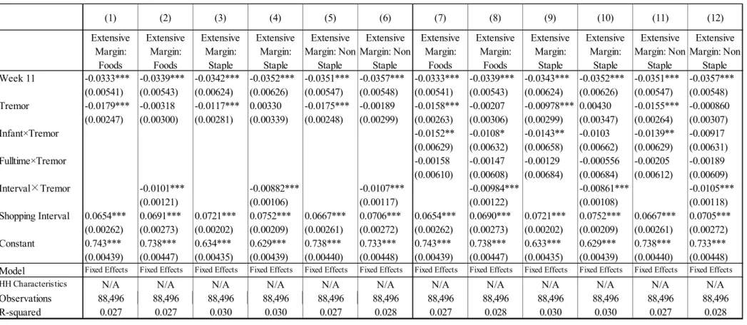
Table 6 presents the estimation results of extensive margins. In all specifications, the number of
major tremors has negative effects on extensive margins12. It implies that the 3/11 disaster reduced the probability of households making any purchase. According to specification (3), for staple foods, an increase in the square root of tremors by one reduces the probability of shopping in Week 11 by 1.2%, while an increase in shopping interval by one week increases the probability of shopping by 7.2%. When the interaction term Interval×Tremors is added in specification (4), its coefficient is negative and significant. This means that the 3/11 disaster dampened the positive effects of shopping interval on the probability of shopping. When we examine household characteristics in specifications (7)–(12), the coefficient of Infant×Tremors is negative and significant in most specifications, while the coefficient of Fulltime×Tremors is not significantly different from zero in all specifications.13 In other words, the households with an infant exhibited a greater reduction in the probability of shopping for both staple and non-staple foods in Week 11 in response to the disaster. To summarize, the 3/11 disaster reduced the likelihood of making any purchase in Week 11 for all households on average, and this effect was stronger for the households with an infant (but not for the households with a working wife).
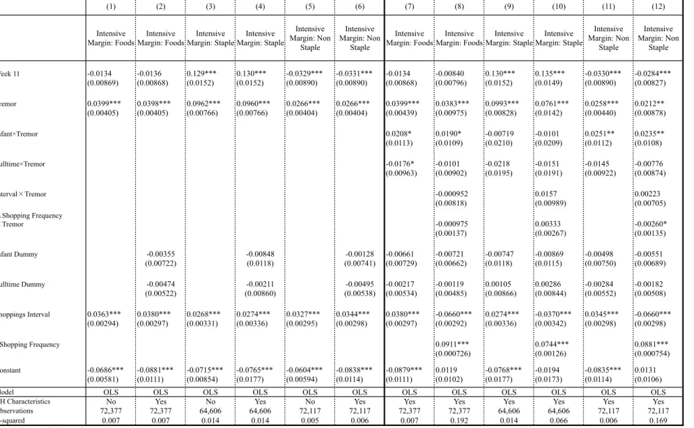
The estimation results of intensive margins are reported in Table 7. In sharp contrast to the extensive margins, in all specifications, the effects of the number of major tremors on intensive margins are positive, large, and significant. In other words, conditional on households making a purchase in Week 11, expenditure was higher for the households experiencing major tremors. In specification (3), for staple foods, an increase in the square root of tremors by one increases the expenditures in Week 11 by 9.6%, while an increase in shopping interval by one week increases the probability of shopping by 2.7%. For all foods in specifications (7) and (8), the coefficient of Infant×Tremors is positive and significant, while that of Fulltime×Tremors is negative and significant. When we decompose foods into staple and non-staple foods, the coefficient of
Infant×Tremors is effectively zero for staple foods (see specifications (9) and (10)), but positive
and significant for non-staple foods (see specifications (11) and (12)). By contrast, the
12 Although the effect of tremors turns positive in specifications (4) and (10), it does not imply that the
disaster raised the probability of shopping. Rather, the negative effect of the interaction term
Interval×Tremors dominates the effect of tremors, as the minimum value of shopping interval is one. 13 Note that, because we include household fixed effects, the effects of household characteristics are
14
coefficients of Fulltime×Tremors are negative but not significant for both staple and non-stale foods. These results suggest that, in response to tremors, conditional on household making a purchase, the households with an infant increased the expenditure on non-staple foods (but not on staple foods) more than the average household did, whereas the households with a working wife increased their food expenditures to a smaller extent than the average households.
To summarize our regression results, the experience of major tremors has positive impacts on the change in the average expenditure in Week 11 and on the expenditure conditional on making a purchase, but negative impacts on the probability of making a purchase during Week 11. Together, it implies that after the disaster some households did not make any purchase of foods at all while other households went shopping and purchased more foods than the pre-disaster level. Unfortunately, we cannot distinguish from the data whether those households who did not make any purchases did so because (a) they did not need to shop, (b) they could not go shopping (due to higher opportunity costs), or (c) they went shopping but could not buy desired goods (because they were sold out). Upon looking into household heterogeneity in response to the disaster, we find that, for the households with a wife working full-time, their probability of purchasing any foods in Week 11 in response to tremors was no lower than the average households, but conditional of purchasing, the increases in their food expenditure were smaller in general. For the households with an infant, they were more likely to make no purchase in Week 11 in response to major tremors, but conditional on purchasing, their expenditures on non-staple goods were greater. Assuming that these households have higher opportunity costs of shopping or higher costs of searching for goods, they most likely fall in the category (b) or (c). If a number of households were “rationed out” despite their willingness to purchase being high, it may have important welfare implications.
6. Concluding Remarks
One year has passed since the Great East Japan Earthquake, and yet, we are far from understanding its wide and profound impact on the Japanese economy. The number of serious empirical studies on the subject has been limited, owing largely to the difficulty in obtaining data. In this paper, we use rich high-frequency micro data to investigate the short-run effects of the 3/11 disaster on consumer purchasing behavior. We find strong evidence of stockpiling, but at the same time, our results suggest that the disaster might have created a measurable discrepancy between households who could stockpile staple foods and those who could not.
15
References
Abe, N., and T. Niizeki (2010), “Household Consumption based on Japanese Homescan Data (in Japanese),” Economic Review, 61(3): 224-236.
Abe, N., C. Moriguchi, and N. Inakura (2012). “The Effects of the Great East Japan Earthquake on Commodity Prices,” mimeo., Institute of Economic Research, Hitotsubashi University. Aguiar, M. and E. Hurst (2007) “Life-Cycle Prices and Production,” American Economic
Review, 97(5): 1533-59.
Batabyal, A. A., G. J. DeAngelo (2012). “Goods Allocation by Queuing and the Occurrence of Violence: A Probabilistic Analysis,” International Review of Economics and Finance, 24: 1-7. Erdem, T., S. Imai, and M. P. Keane (2003). “Brand and Quantity Choice Dynamics under Price Uncertainty,” Quantitative Marketing and Economics, 1(1): 5-64.
Hendel, I. and A. Nevo (2006a). “Sales and Consumer Inventory,” Rand Journal of Economics, 37(3): 543–561.
Hendel, I. and A. Nevo (2006b). “Measuring the Implications of Sales and Consumer Stockpiling Behavior,” Econometrica, 74(6): 1637-1673.
Ivancic, L., E. W. Diewert, and K. J. Fox, (2011) “Scanner data, Time Aggregation and the Construction of Price Indexes,” Journal of Econometrics, 161(1): 24-35.
Table 1: Comparisons of Changes in Price Indexes in Week 11
Note: Standard deviations are in parentheses.
t-statistics for the mean differences between East and Western part of Japan are reported.
*: significant at 10 %.
The base period for the Laspyres index is Week 9.
Staple foods include rice, bread, noodle, cereal, flour, and pancake mix.
East West t-statistics Laspyres 0.0186 -0.0045 1.35 (0.016) (0.007) Paasche 0.0266 -0.0057 1.40 (0.021) (0.008) Fisher 0.0226 -0.0051 1.40 (0.018) (0.007) Laspyres 0.0376 -0.0185 1.34 (0.037) (0.021) Pasache 0.0441 -0.0451 1.72* (0.045) (0.026) Fisher 0.0408 -0.0316 1.56 (0.041) (0.023) Laspyres 0.0147 0.0014 1.22 (0.009) (0.006) Pasache 0.0207 0.0063 1.52 (0.008) (0.005) Fisher 0.0177 0.0039 1.42 (0.008) (0.005) Foods Staple Foods Non Staple Foods
Table 2: Descriptive Statistics of Weekly Expenditures on Foods
Note: Staple foods include rice, bread, noodle, cereal, flour, and pancake mix. The 3/11 is the first day of Week 11.
Foods Staple Else Foods Staple Else Foods Staple Else Food Staple Else Foods Staple Else Food Staple Else 2 3853 3504 726 2777 3291 1127 2681 5063 3228 667 2561 3074 1011 2530 11312 3336 689 2647 3149 1055 2583 3 3853 3580 729 2852 3340 1050 2767 5063 3476 697 2779 3174 1048 2611 11312 3533 716 2816 3271 1082 2696 4 3853 3716 744 2972 3582 1099 2978 5063 3583 712 2871 3415 1016 2856 11312 3644 726 2918 3458 1066 2883 5 3853 4189 838 3351 3994 1240 3294 5063 3818 754 3065 3499 1077 2914 11312 3967 789 3178 3725 1179 3069 6 3853 3780 760 3020 3620 1056 3028 5063 3438 706 2731 3251 1055 2677 11312 3568 720 2848 3398 1057 2817 7 3853 3687 773 2915 3532 1134 2878 5063 3512 711 2801 3409 1189 2793 11312 3606 743 2863 3459 1169 2825 8 3853 3719 785 2933 3535 1133 2868 5063 3510 733 2778 3269 1111 2696 11312 3590 751 2839 3405 1141 2777 9 3853 4325 892 3433 4064 1292 3345 5063 3987 798 3189 3707 1204 3067 11312 4100 830 3270 3869 1285 3196 10 3853 3672 800 2872 3471 1164 2800 5063 3382 712 2671 3245 1072 2610 11312 3485 737 2749 3317 1097 2691 11 3853 4472 1287 3184 4492 1780 3256 5063 3472 793 2679 3318 1139 2672 11312 3922 1013 2908 3913 1533 2955 12 3853 3477 880 2598 3762 1458 2860 5063 3366 730 2636 3341 1103 2738 11312 3391 785 2606 3502 1275 2767 13 3853 3790 826 2964 4143 1453 3299 5063 3736 774 2963 3761 1267 3057 11312 3741 790 2950 3920 1334 3156 14 3853 3236 649 2587 3353 1007 2773 5063 3129 655 2474 3213 1198 2600 11312 3170 650 2519 3268 1137 2670 15 3853 3640 740 2900 3539 1127 2881 5063 3309 678 2631 3213 1062 2644 11312 3445 702 2743 3359 1153 2727 16 3853 3595 749 2846 3463 1131 2786 5063 3441 709 2732 3214 1017 2665 11312 3496 721 2775 3310 1075 2708 17 3853 3799 784 3015 3757 1154 3074 5063 3698 759 2939 3473 1154 2863 11312 3716 761 2955 3596 1169 2959 18 3853 3738 764 2975 3961 1255 3278 5063 3512 731 2780 3653 1163 2983 11312 3610 740 2871 3793 1198 3119 19 3853 3483 703 2780 3473 1044 2844 5063 3356 690 2665 3315 1042 2731 11312 3396 692 2704 3346 1062 2742 20 3853 3681 750 2931 3446 1115 2815 5063 3419 707 2712 3246 1016 2683 11312 3514 726 2788 3334 1142 2716 21 3853 4019 828 3191 3857 1153 3149 5063 3767 772 2995 3472 1095 2877 11312 3827 786 3041 3608 1140 2961 Total 77060 3755 800 2955 3707 1218 2997 101260 3507 724 2783 3374 1105 2773 226240 3603 753 2849 3514 1175 2861 Std.dev N Mean Week
East West All
Std.dev
Table 3: Covariance Structure of Change Rate of Expenditures in Weeks 2-10 before 3/11
Note: The first differences in household expenditures on foods, staple foods, and non-staple foods. The upper triangle shows the variance and covariance, while the lower triangle shows the correlation. The sample period covers Week 2-10.
Foods
dln(Expense) dln(Expense)[-1] dln(Expense)[-2] dln(Expense)[-3] dln(Expense)[-4] dln(Expense)[-5]
dln(Expense) 0.6525 -0.3491 0.0219 -0.0118 0.0208 -0.0046 dln(Expense)[-1] -0.5402 0.6399 -0.3415 0.0309 -0.0061 0.0077 dln(Expense)[-2] 0.0338 -0.5339 0.6393 -0.3577 0.0265 0.0032 dln(Expense)[-3] -0.0181 0.0478 -0.5546 0.6508 -0.3516 0.0200 dln(Expense)[-4] 0.0320 -0.0094 0.0412 -0.5418 0.6471 -0.3440 dln(Expense)[-5] -0.0072 0.0120 0.0049 0.0310 -0.5336 0.6421 Number of observarions = 16726 Staple Foods
dln(Expense) dln(Expense)[-1] dln(Expense)[-2] dln(Expense)[-3] dln(Expense)[-4] dln(Expense)[-5]
dln(Expense) 1.3806 -0.7584 0.0671 -0.0452 0.0722 -0.0296 dln(Expense)[-1] -0.5532 1.3613 -0.7372 0.0755 -0.0328 0.0396 dln(Expense)[-2] 0.0494 -0.5463 1.3374 -0.7458 0.0735 -0.0194 dln(Expense)[-3] -0.0331 0.0556 -0.5546 1.3521 -0.7458 0.0792 dln(Expense)[-4] 0.0529 -0.0242 0.0547 -0.5518 1.3508 -0.7481 dln(Expense)[-5] -0.0217 0.0292 -0.0144 0.0587 -0.5545 1.3477 Number of observarions = 11267 Non-Staple Foods
dln(Expense) dln(Expense)[-1] dln(Expense)[-2] dln(Expense)[-3] dln(Expense)[-4] dln(Expense)[-5]
dln(Expense) 0.7081 -0.3702 0.0191 -0.0203 0.0290 -0.0041 dln(Expense)[-1] -0.5299 0.6890 -0.3627 0.0296 -0.0123 0.0116 dln(Expense)[-2] 0.0272 -0.5244 0.6943 -0.3837 0.0232 0.0060 dln(Expense)[-3] -0.0287 0.0424 -0.5475 0.7072 -0.3793 0.0180 dln(Expense)[-4] 0.0410 -0.0177 0.0332 -0.5368 0.7060 -0.3720 dln(Expense)[-5] -0.0059 0.0167 0.0086 0.0256 -0.5304 0.6967 Number of observarions = 16538
Table 4: Descriptive Statistics
Note: Sample statistics of the variables used in Tables 5, 6 and 7. Sample Periods: Week 4 - 11.
Number of tremors is the number of major tremors (more than 3 in seismic scale) observed in each prefecture each week. See the main text for definitions of other variables.
N Mean St.d. Min Max
88496 0.1728 0.6511 0 4.7958 88496 0.1246 0.3303 0 1 88496 0.1445 0.3516 0 1 88496 2.9550 2.5751 0 23 88496 -0.0427 2.3417 -19 19 Foods 88496 1.3607 1.0562 1 10 Staple Foods 88496 1.5558 1.2695 1 10
Non Staple Foods 88496 1.3654 1.0601 1 10
88496 0.0212 0.2363 0 4.7958
88496 0.0230 0.2441 0 4.7958
88496 -0.0185 1.5601 -48 34.8569
Foods 88496 0.2487 1.3269 0 47.9583
Staple Foods 88496 0.2895 1.5691 0 47.9583
Non Staple Foods 88496 0.2496 1.3310 0 47.9583
Shopping Interval of Tremors×Infant Tremors×Fulltime Tremors×Δshoppings Tremors× Interval of Δshoppings Sqrt (Frequency of Tremors) Infant Dummy Fulltime Dummy Number of Shoppings
(1) (2) (3) (4) (5) (6) (7) (8) (9) (10) (11) (12) Δ Foods Δ Foods Δ Staple Δ Staple Δ Non Staple Δ Non Staple Δ Foods Δ Foods Δ Staple Δ Staple Δ Non Staple Δ Non Staple
Week 11 -120.0** -120.5** 23.94 23.99 -144.0*** -144.5*** -120.7** -49.01 23.83 38.62** -144.6*** -87.62** (57.50) (57.51) (21.32) (21.33) (47.14) (47.15) (57.51) (44.15) (21.33) (19.69) (47.15) (37.45) Tremor 68.55*** 68.77*** 52.73*** 52.70*** 15.82 16.07 83.88*** 97.41*** 62.68*** 66.34*** 21.20 31.07* (25.16) (25.17) (8.843) (8.843) (20.81) (20.82) (28.13) (21.65) (9.923) (9.193) (23.24) (18.48) Infant × Tremor 16.56 13.88 -26.25 -27.09* 42.81 40.98 (50.16) (42.13) (17.19) (16.22) (41.08) (35.02) Fulltime × Tremor -128.3** -69.14 -50.11** -36.49* -78.14* -32.64 (57.46) (45.57) (21.12) (19.68) (47.46) (38.75) ΔShopping Frequency Tremor -10.65 4.256 -14.91* (9.169) (3.639) (7.789) Infant Dummy -5.136 -0.242 -4.894 -8.061 -20.64 4.232 1.597 -12.29 -22.24 (44.43) (14.73) (36.88) (45.53) (34.75) (15.04) (13.92) (37.84) (29.50) Fulltime Dummy -11.23 -2.474 -8.758 9.434 10.07 5.608 5.721 3.826 4.346 (38.27) (13.58) (31.49) (39.52) (30.33) (13.94) (12.88) (32.56) (25.69) ΔShopping Frequency 1,077*** 227.2*** 849.8*** (6.292) (2.490) (5.307) Constant 40.97 66.55 -5.760 -2.950 46.73 69.50 64.37 45.34 -4.505 -8.537 68.88 53.88 (34.57) (61.77) (12.60) (21.23) (28.76) (51.85) (61.82) (47.49) (21.25) (19.85) (51.88) (40.88)
Model OLS OLS OLS OLS OLS OLS OLS OLS OLS OLS OLS OLS
HH Characteristics No Yes No Yes No Yes Yes Yes Yes Yes Yes Yes
Observations 88,496 88,496 88,496 88,496 88,496 88,496 88,496 88,496 88,496 88,496 88,496 88,496
R-squared 0.008 0.009 0.003 0.003 0.008 0.008 0.009 0.419 0.003 0.145 0.008 0.384
Tremor is the square root of the number of major tremors.
Week dummies are included in all the specifications. Week 4 = base week. March 11 is the first day of Week 11.
HH Characteristics: Dummies for the size of households, dummies for six income categories, dummies for eight categories of wife's age, infant dummy, and fulltime-working wife dummy. Staple food include rice, bread, noodles, cereal, flour, and pancake mix.
Table 5: The Effects of The 3/11 Disaster on the First Differences in Expenditures
Note: Robust standard errors in parentheses. *** p<0.01, ** p<0.05, * p<0.1
Dependent variables are the first differences in expenditures. Sample Periods: Weeks 4 - 11 in 2011.
Table 6: The Effects of The 3/11 Disaster on the Extensive Margins of Expenditures
Note: Robust standard errors in parentheses.
*** p<0.01, ** p<0.05, * p<0.1
Dependent variables are the dummy variables for positive expenditures. See the note for Table 5 for the detailed explanations.
(1) (2) (3) (4) (5) (6) (7) (8) (9) (10) (11) (12) Extensive Margin: Foods Extensive Margin: Foods Extensive Margin: Staple Extensive Margin: Staple Extensive Margin: Non Staple Extensive Margin: Non Staple Extensive Margin: Foods Extensive Margin: Foods Extensive Margin: Staple Extensive Margin: Staple Extensive Margin: Non Staple Extensive Margin: Non Staple Week 11 -0.0333*** -0.0339*** -0.0342*** -0.0352*** -0.0351*** -0.0357*** -0.0333*** -0.0339*** -0.0343*** -0.0352*** -0.0351*** -0.0357*** (0.00541) (0.00543) (0.00624) (0.00626) (0.00547) (0.00548) (0.00541) (0.00543) (0.00624) (0.00626) (0.00547) (0.00548) Tremor -0.0179*** -0.00318 -0.0117*** 0.00330 -0.0175*** -0.00189 -0.0158*** -0.00207 -0.00978*** 0.00430 -0.0155*** -0.000860 (0.00247) (0.00300) (0.00281) (0.00339) (0.00248) (0.00299) (0.00263) (0.00306) (0.00299) (0.00347) (0.00264) (0.00307) Infant×Tremor -0.0152** -0.0108* -0.0143** -0.0103 -0.0139** -0.00917 (0.00629) (0.00632) (0.00658) (0.00662) (0.00629) (0.00631) Fulltime×Tremor -0.00158 -0.00147 -0.00129 -0.000556 -0.00205 -0.00189 (0.00610) (0.00608) (0.00684) (0.00684) (0.00612) (0.00609) Interval×Tremor -0.0101*** -0.00882*** -0.0107*** -0.00984*** -0.00861*** -0.0105*** (0.00121) (0.00106) (0.00117) (0.00122) (0.00108) (0.00118) Shopping Interval 0.0654*** 0.0691*** 0.0721*** 0.0752*** 0.0667*** 0.0706*** 0.0654*** 0.0690*** 0.0721*** 0.0752*** 0.0667*** 0.0705*** (0.00262) (0.00273) (0.00202) (0.00209) (0.00261) (0.00272) (0.00262) (0.00273) (0.00202) (0.00209) (0.00261) (0.00272) Constant 0.743*** 0.738*** 0.634*** 0.629*** 0.738*** 0.733*** 0.743*** 0.738*** 0.633*** 0.629*** 0.738*** 0.733*** (0.00439) (0.00447) (0.00435) (0.00439) (0.00440) (0.00448) (0.00439) (0.00447) (0.00435) (0.00439) (0.00440) (0.00448) Model Fixed Effects Fixed Effects Fixed Effects Fixed Effects Fixed Effects Fixed Effects Fixed Effects Fixed Effects Fixed Effects Fixed Effects Fixed Effects Fixed Effects
HH Characteristics N/A N/A N/A N/A N/A N/A N/A N/A N/A N/A N/A N/A Observations 88,496 88,496 88,496 88,496 88,496 88,496 88,496 88,496 88,496 88,496 88,496 88,496 R-squared 0.027 0.027 0.030 0.030 0.027 0.028 0.027 0.028 0.030 0.030 0.027 0.028
(1) (2) (3) (4) (5) (6) (7) (8) (9) (10) (11) (12) Intensive
Margin: FoodsMargin: FoodsIntensive Margin: StapleIntensive Margin: StapleIntensive
Intensive Margin: Non Staple Intensive Margin: Non Staple Intensive
Margin: FoodsMargin: FoodsIntensive Margin: StapleIntensive Margin: StapleIntensive
Intensive Margin: Non Staple Intensive Margin: Non Staple Week 11 -0.0134 -0.0136 0.129*** 0.130*** -0.0329*** -0.0331*** -0.0134 -0.00840 0.130*** 0.135*** -0.0330*** -0.0284*** (0.00869) (0.00868) (0.0152) (0.0152) (0.00890) (0.00890) (0.00868) (0.00796) (0.0152) (0.0149) (0.00890) (0.00827) Tremor 0.0399*** 0.0398*** 0.0962*** 0.0960*** 0.0266*** 0.0266*** 0.0399*** 0.0383*** 0.0993*** 0.0761*** 0.0258*** 0.0212** (0.00405) (0.00405) (0.00766) (0.00766) (0.00404) (0.00404) (0.00439) (0.00975) (0.00828) (0.0142) (0.00440) (0.00878) Infant×Tremor 0.0208* 0.0190* -0.00719 -0.0101 0.0251** 0.0235** (0.0113) (0.0109) (0.0210) (0.0209) (0.0112) (0.0108) Fulltime×Tremor -0.0176* -0.0101 -0.0218 -0.0151 -0.0145 -0.00776 (0.00963) (0.00902) (0.0195) (0.0191) (0.00922) (0.00874) Interval Tremor -0.000952 0.0157 0.00223 (0.00818) (0.00989) (0.00705) ΔShopping Frequency Tremor -0.000975 0.00333 -0.00260* (0.00137) (0.00267) (0.00135) Infant Dummy -0.00355 -0.00848 -0.00128 -0.00661 -0.00721 -0.00747 -0.00869 -0.00498 -0.00551 (0.00722) (0.0118) (0.00741) (0.00729) (0.00662) (0.0118) (0.0115) (0.00750) (0.00689) Fulltime Dummy -0.00474 -0.00211 -0.00495 -0.00217 -0.00119 0.00105 0.00286 -0.00284 -0.00182 (0.00522) (0.00860) (0.00538) (0.00534) (0.00485) (0.00866) (0.00844) (0.00552) (0.00508) Shoppings Interval 0.0363*** 0.0380*** 0.0268*** 0.0274*** 0.0327*** 0.0344*** 0.0380*** -0.0660*** 0.0274*** -0.0370*** 0.0345*** -0.0660*** (0.00294) (0.00297) (0.00331) (0.00336) (0.00295) (0.00298) (0.00297) (0.00292) (0.00336) (0.00342) (0.00298) (0.00298) ΔShopping Frequency 0.0911*** 0.0744*** 0.0881*** (0.000726) (0.00126) (0.000754) Constant -0.0686*** -0.0881*** -0.0715*** -0.0765*** -0.0604*** -0.0838*** -0.0879*** 0.0119 -0.0768*** -0.0194 -0.0835*** 0.0131 (0.00581) (0.0111) (0.00854) (0.0177) (0.00594) (0.0114) (0.0111) (0.0102) (0.0177) (0.0173) (0.0114) (0.0106)
Model OLS OLS OLS OLS OLS OLS OLS OLS OLS OLS OLS OLS
HH Characteristics No Yes No Yes No Yes Yes Yes Yes Yes Yes Yes
Observations 72,377 72,377 64,606 64,606 72,117 72,117 72,377 72,377 64,606 64,606 72,117 72,117
R-squared 0.007 0.007 0.014 0.014 0.005 0.006 0.007 0.192 0.014 0.066 0.006 0.169
Dependent Variables are the ratio of the gap between actual and average expenditures divided by the average expenditures. Observations with zero expenditures are excluded.
Table 7: The Effects of The 3/11 Disaster on The Intensive Margins of Expenditures
Note: Robust standard errors in parentheses. *** p<0.01, ** p<0.05, * p<0.1
Figure 1-(a
Figure 1-(b
Figure 1-(C
a): The Fre
b): The Fre
C): The Fre
equency of
equency of
equency of
Major Trem
Major Trem
f Major Tre
mors in We
mors in We
emors in W
eeks 8-9
eeks 11-12
Weeks 13-14
F
Figure 3: Daily Expenditures on Foods
0 200 400 600 800 1000 1200 1400 1600 1800 2000 0 500 1000 1500 2000 2500 8-Ja n 15 -Jan 22 -Jan 29 -Jan 5-Feb 12 -F eb 19 -F eb 26 -F eb 5-M ar 12 -Mar 19 -Mar 26 -Mar 2-A pr 9-A pr 16 -Apr 23 -Apr 30 -Apr 7-M ay 14 -M ay 21 -M ayEast West (Right Axis)
¥1000 ¥1000
Figure 4: Weekly Expenditures on Foods
Figure 5: Fisher Price Index for Foods
0.85 0.9 0.95 1 1.05 1.1 1.15 1.2 1.25 2 3 4 5 6 7 8 9 10 11 12 13 14 15 16 17 18 19 20 21Hokkaido Tokyo Osaka Fukuoka
0.96 0.97 0.98 0.99 1 1.01 1.02 1.03 1.04 1.05 1.06 2 3 4 5 6 7 8 9 10 11 12 13 14 15 16 17 18 19 20 21
Figure 6: Expenditures on Several Categories
Storable Goods Perishable Goods
0 0.5 1 1.5 2 2.5 3 3.5 2 3 4 5 6 7 8 9 10 11 12 13 14 15 16 17 18 19 20 (b) Cereal East West 0 0.5 1 1.5 2 2.5 3 2 3 4 5 6 7 8 9 10 11 12 13 14 15 16 17 18 19 20 (c) Flour East West 0 0.2 0.4 0.6 0.8 1 1.2 1.4 2 3 4 5 6 7 8 9 10 11 12 13 14 15 16 17 18 19 20 (d) Bread East West 0 0.2 0.4 0.6 0.8 1 1.2 1.4 2 3 4 5 6 7 8 9 10 11 12 13 14 15 16 17 18 19 20 (e) Tofu East West 0 0.2 0.4 0.6 0.8 1 1.2 1.4 2 3 4 5 6 7 8 9 10 11 12 13 14 15 16 17 18 19 20 (f) Ham East West 0 0.5 1 1.5 2 2 3 4 5 6 7 8 9 10 11 12 13 14 15 16 17 18 19 20 (a) Rice East West
Appendix Table 1: Weekly Frequency of Tremors whose Seismic Scale Is Greater Than 3.
Note: No major earthquakes occurred during in Week 2, 3, 4, and 7. Source: Japan Meteorological Agency
pref_code Prefecture Name 5 6 7 8 9 10 11 12 13 14 15 16 17 18 19 20 21
1 Hokkaido 0 0 0 0 0 0 4 0 0 1 0 0 0 0 0 0 0 2 Aomori 0 0 0 0 0 1 9 0 1 2 0 1 0 0 0 0 0 3 Iwate 0 0 0 0 0 1 27 3 4 4 3 0 0 1 1 0 0 4 Miyagi 0 0 0 0 0 2 30 8 5 5 3 1 3 0 0 0 0 5 Akita 0 0 0 0 0 1 8 1 0 2 1 1 0 0 0 0 0 6 Yamagata 0 0 0 0 0 1 13 0 1 1 2 0 1 0 0 0 0 7 Fukushima 0 1 0 0 0 1 37 8 4 4 19 4 4 4 2 3 2 8 Ibaraki 0 0 0 0 0 0 37 9 2 5 11 3 3 1 1 0 4 9 Tochigi 0 0 0 0 0 0 16 6 0 2 5 2 1 0 0 0 0 10 Gumma 0 0 0 0 0 0 5 1 0 2 3 1 1 0 0 0 0 11 Saitama 0 0 0 0 0 0 10 2 0 2 4 2 0 0 0 0 0 12 Chiba 0 1 0 0 0 0 15 3 0 2 3 2 1 0 0 0 2 13 Tokyo 0 0 0 0 0 0 4 0 0 0 2 1 0 0 0 0 0 14 Kanagawa 0 0 0 0 0 0 4 0 0 0 1 0 0 0 0 0 0 15 Niigata 0 0 0 0 0 0 10 0 0 1 2 1 0 0 0 0 0 16 Toyama 0 0 0 0 0 0 0 0 0 0 0 0 0 0 0 0 0 17 Ishikawa 0 0 0 0 0 0 1 0 0 0 0 0 0 0 0 0 0 18 Fukui 0 0 0 0 0 0 0 0 0 0 0 0 0 0 0 0 0 19 Yamanashi 0 0 0 0 0 0 3 0 0 0 0 0 0 0 0 0 0 20 Nagano 0 0 0 0 0 0 23 0 1 0 2 0 0 0 0 0 0 21 Gifu 0 0 0 0 2 0 3 0 0 0 0 0 0 0 0 0 0 22 Shizuoka 1 0 0 0 0 0 5 0 0 0 0 0 0 0 0 0 0 23 Aichi 0 0 0 0 0 0 1 0 0 0 0 0 0 0 0 0 0 24 Mie 0 0 0 0 0 0 0 0 0 0 0 0 0 0 0 0 0 25 Saga 0 0 0 0 0 0 0 0 0 0 0 0 0 0 0 0 0 26 Kyoto 0 0 0 0 0 0 0 0 0 0 0 0 0 0 0 0 0 27 Osaka 0 0 0 0 0 0 0 0 0 0 0 0 0 0 0 0 0 28 Hyogo 0 0 0 0 0 0 0 0 0 0 0 0 0 0 0 0 0 29 Nara 0 0 0 0 0 0 0 0 0 0 0 0 0 0 0 0 0 30 Wakayama 0 0 0 1 0 0 0 0 0 0 0 0 0 0 1 0 0 31 Tottori 0 0 0 0 0 0 0 0 0 0 0 0 0 0 0 0 0 32 Shimane 0 0 0 0 0 0 0 0 0 0 0 0 0 0 0 0 0 33 Okayama 0 0 0 0 0 0 0 0 0 0 0 0 0 0 0 0 0 34 Hiroshima 0 0 0 0 0 0 0 0 0 0 0 0 0 0 0 0 0 35 Yamaguchi 0 0 0 0 0 0 0 0 0 0 0 0 0 0 0 0 0 36 Tokushima 0 0 0 0 0 0 0 0 0 0 0 0 0 0 0 0 0 37 Kagawa 0 0 0 0 0 0 0 0 0 0 0 0 0 0 0 0 0 38 Ehime 0 0 0 0 0 0 0 0 0 0 0 0 0 0 0 0 0 39 Kochi 0 0 0 0 0 0 0 0 0 0 0 0 0 0 0 0 0 40 Fukuoka 0 0 0 0 0 0 0 0 0 0 0 0 0 0 0 0 0 41 Saga 0 0 0 0 0 0 0 0 0 0 0 0 0 0 0 0 0 42 Nagasaki 0 0 0 0 0 0 0 0 0 0 0 0 0 0 0 0 0 43 Kumamoto 0 0 0 0 0 0 0 0 0 0 0 0 0 0 0 0 0 44 Oita 0 0 0 0 0 0 0 0 0 0 0 0 0 0 0 0 0 45 Miyazaki 0 0 0 0 0 0 0 0 0 0 0 0 0 0 0 0 0 46 Kagoshimia 0 0 0 0 0 0 0 0 0 0 0 0 0 0 0 0 0 week
Appendix Table 2: Movements of ln(Expenditures) on Staple Foods
Week N mean sd N mean sd N mean sd
2 2791 6.41 1.00 3670 6.34 0.99 8174 6.37 1.00 3 2787 6.42 1.02 3748 6.38 0.97 8317 6.39 1.00 4 2771 6.43 1.04 3789 6.39 0.98 8330 6.40 1.01 5 2882 6.49 1.05 3887 6.39 1.02 8546 6.43 1.04 6 2780 6.49 1.00 3710 6.39 0.99 8229 6.41 1.00 7 2796 6.47 1.02 3710 6.39 1.00 8255 6.42 1.01 8 2775 6.49 1.03 3743 6.41 0.99 8251 6.43 1.02 9 2903 6.54 1.06 3931 6.42 1.02 8623 6.46 1.04 10 2786 6.51 1.03 3697 6.41 0.98 8208 6.43 1.00 11 2727 7.01 1.07 3718 6.49 1.01 8167 6.71 1.07 12 2555 6.66 1.05 3670 6.42 1.00 7860 6.50 1.03 13 2695 6.51 1.06 3745 6.41 1.03 8134 6.45 1.05 14 2512 6.43 0.99 3505 6.35 1.01 7642 6.37 1.00 15 2724 6.46 1.00 3710 6.35 0.99 8130 6.39 1.00 16 2708 6.46 1.03 3687 6.41 0.99 8105 6.42 1.01 17 2782 6.49 1.02 3816 6.42 1.00 8310 6.43 1.02 18 2627 6.50 1.03 3509 6.45 1.02 7764 6.46 1.03 19 2667 6.43 1.02 3694 6.37 0.98 8029 6.39 1.00 20 2716 6.49 0.99 3715 6.39 0.99 8155 6.42 1.00 21 2837 6.54 1.02 3846 6.46 0.99 8396 6.47 1.02 54821 6.51 1.03 74500 6.40 1.00 163625 6.44 1.02
week N mean sd min max N mean sd min max N mean sd min max 2 3853 2.94 2.54 0 15 5063 2.86 2.44 0 20 11312 2.83 2.44 0 20 3 3853 2.99 2.62 0 19 5063 3.00 2.55 0 22 11312 2.94 2.53 0 22 4 3853 3.04 2.68 0 18 5063 3.04 2.61 0 19 11312 2.98 2.58 0 19 5 3853 3.25 2.71 0 19 5063 3.13 2.59 0 22 11312 3.13 2.60 0 22 6 3853 3.07 2.75 0 20 5063 2.97 2.59 0 23 11312 2.94 2.60 0 23 7 3853 2.93 2.60 0 18 5063 2.93 2.54 0 21 11312 2.90 2.54 0 21 8 3853 3.00 2.63 0 18 5063 3.01 2.58 0 19 11312 2.94 2.56 0 20 9 3853 3.30 2.69 0 18 5063 3.20 2.59 0 19 11312 3.18 2.59 0 19 10 3853 3.00 2.68 0 19 5063 2.93 2.57 0 23 11312 2.91 2.58 0 23 11 3853 3.13 2.92 0 21 5063 2.94 2.56 0 18 11312 2.97 2.67 0 21 12 3853 2.85 2.81 0 22 5063 2.81 2.51 0 17 11312 2.77 2.58 0 22 13 3853 3.07 2.83 0 22 5063 2.98 2.57 0 21 11312 2.95 2.63 0 22 14 3853 2.82 2.80 0 24 5063 2.80 2.60 0 22 11312 2.75 2.62 0 24 15 3853 3.01 2.74 0 21 5063 2.93 2.54 0 19 11312 2.91 2.58 0 21 16 3853 3.04 2.78 0 21 5063 3.01 2.63 0 17 11312 2.97 2.63 0 21 17 3853 3.06 2.72 0 18 5063 3.06 2.61 0 19 11312 2.99 2.62 0 19 18 3853 2.84 2.71 0 17 5063 2.82 2.61 0 21 11312 2.78 2.59 0 21 19 3853 2.92 2.66 0 21 5063 2.92 2.53 0 19 11312 2.87 2.55 0 21 20 3853 3.03 2.75 0 19 5063 2.99 2.59 0 19 11312 2.95 2.61 0 19 21 3853 3.15 2.75 0 20 5063 3.14 2.60 0 18 11312 3.06 2.62 0 20 Total 77060 3.02 2.72 0 24 101260 2.97 2.57 0 23 226240 2.94 2.59 0 24
Appendix Table 3: Weekly Shopping Frequencies
Appendix Table 4: Shopping Interval (in Weeks)
Note: The shopping interval from the last purchase. In each week, only households with positive purchases are included when calculation this table.
week
N mean sd N mean sd N mean sd N mean sd N mean sd N mean sd
2 3158 1 0 2791 1 0 3140 1 0 4099 1 0 3670 1 0 4086 1 0 3 3136 1.10 0.30 2787 1.18 0.38 3127 1.11 0.31 4172 1.11 0.32 3748 1.18 0.39 4159 1.12 0.32 4 3143 1.15 0.44 2771 1.25 0.57 3130 1.15 0.45 4194 1.16 0.47 3789 1.25 0.58 4179 1.16 0.47 5 3283 1.25 0.69 2882 1.36 0.80 3262 1.25 0.70 4294 1.20 0.61 3887 1.30 0.72 4279 1.20 0.61 6 3119 1.14 0.51 2780 1.28 0.74 3104 1.14 0.52 4092 1.14 0.50 3710 1.26 0.73 4077 1.14 0.51 7 3125 1.16 0.54 2796 1.29 0.77 3113 1.17 0.56 4121 1.16 0.55 3710 1.26 0.71 4108 1.17 0.55 8 3148 1.19 0.61 2775 1.31 0.81 3142 1.19 0.62 4176 1.20 0.64 3743 1.30 0.80 4166 1.20 0.65 9 3279 1.28 0.89 2903 1.47 1.20 3265 1.28 0.90 4389 1.28 0.94 3931 1.43 1.14 4377 1.29 0.94 10 3099 1.17 0.72 2786 1.30 0.91 3088 1.17 0.72 4112 1.14 0.68 3697 1.28 0.90 4096 1.15 0.68 11 2960 1.15 0.56 2727 1.30 0.87 2949 1.15 0.58 4101 1.15 0.56 3718 1.27 0.78 4077 1.16 0.57 12 2907 1.20 0.59 2555 1.29 0.77 2889 1.20 0.60 4055 1.17 0.54 3670 1.31 0.87 4039 1.17 0.55 13 3067 1.40 1.12 2695 1.56 1.33 3054 1.40 1.12 4192 1.28 0.87 3745 1.43 1.16 4172 1.28 0.87 14 2893 1.30 1.20 2512 1.41 1.24 2875 1.31 1.20 3922 1.25 1.13 3505 1.37 1.22 3908 1.25 1.13 15 3092 1.24 0.72 2724 1.42 1.06 3079 1.25 0.73 4125 1.20 0.64 3710 1.33 0.88 4107 1.21 0.66 16 3098 1.20 0.71 2708 1.37 0.99 3086 1.21 0.73 4080 1.18 0.72 3687 1.31 0.93 4067 1.19 0.73 17 3124 1.23 0.77 2782 1.42 1.14 3113 1.25 0.81 4248 1.24 0.82 3816 1.37 1.10 4238 1.24 0.83 18 2977 1.32 1.40 2627 1.46 1.54 2962 1.32 1.34 3941 1.29 1.35 3509 1.44 1.57 3917 1.29 1.35 19 3052 1.24 0.81 2667 1.40 1.16 3038 1.25 0.92 4105 1.24 0.95 3694 1.40 1.18 4084 1.25 0.94 20 3096 1.21 0.74 2716 1.38 1.10 3087 1.22 0.74 4163 1.18 0.68 3715 1.31 0.87 4150 1.19 0.71 21 3174 1.22 0.78 2837 1.40 1.18 3168 1.22 0.79 4223 1.19 0.70 3846 1.34 0.97 4208 1.19 0.70 Total 61930 1.21 0.77 54821 1.34 0.99 61671 1.21 0.78 82804 1.19 0.74 74500 1.31 0.94 82494 1.19 0.74 East West
Appendix Table 5: The Ratio of HHs with Positive Expenditures
week Foods Staple Non Staple Foods Staple Non Staple Foods Staple Non Staple
2 0.82 0.72 0.81 0.81 0.72 0.81 0.82 0.72 0.81 3 0.81 0.72 0.81 0.82 0.74 0.82 0.82 0.74 0.82 4 0.82 0.72 0.81 0.83 0.75 0.83 0.83 0.74 0.82 5 0.85 0.75 0.85 0.85 0.77 0.85 0.85 0.76 0.84 6 0.81 0.72 0.81 0.81 0.73 0.81 0.81 0.73 0.81 7 0.81 0.73 0.81 0.81 0.73 0.81 0.81 0.73 0.81 8 0.82 0.72 0.82 0.82 0.74 0.82 0.82 0.73 0.82 9 0.85 0.75 0.85 0.87 0.78 0.86 0.86 0.76 0.85 10 0.80 0.72 0.80 0.81 0.73 0.81 0.81 0.73 0.81 11 0.77 0.71 0.77 0.81 0.73 0.81 0.79 0.72 0.79 12 0.75 0.66 0.75 0.80 0.72 0.80 0.78 0.69 0.78 13 0.80 0.70 0.79 0.83 0.74 0.82 0.81 0.72 0.81 14 0.75 0.65 0.75 0.77 0.69 0.77 0.77 0.68 0.76 15 0.80 0.71 0.80 0.81 0.73 0.81 0.81 0.72 0.81 16 0.80 0.70 0.80 0.81 0.73 0.80 0.81 0.72 0.80 17 0.81 0.72 0.81 0.84 0.75 0.84 0.82 0.73 0.82 18 0.77 0.68 0.77 0.78 0.69 0.77 0.78 0.69 0.77 19 0.79 0.69 0.79 0.81 0.73 0.81 0.80 0.71 0.80 20 0.80 0.70 0.80 0.82 0.73 0.82 0.81 0.72 0.81 21 0.82 0.74 0.82 0.83 0.76 0.83 0.83 0.74 0.82 Total 0.80 0.71 0.80 0.82 0.74 0.81 0.81 0.72 0.81
Appendix Table 6: Intensive Margin
Week mean sd mean sd mean sd mean sd mean sd mean sd mean sd mean sd mean sd 2 -0.07 0.44 -0.06 0.68 -0.07 0.45 -0.08 0.44 -0.05 0.65 -0.08 0.45 -0.08 0.44 -0.06 0.67 -0.08 0.45 3 -0.05 0.45 -0.05 0.69 -0.04 0.46 -0.03 0.44 -0.03 0.64 -0.03 0.46 -0.04 0.45 -0.04 0.67 -0.03 0.46 4 -0.03 0.46 -0.06 0.68 -0.02 0.48 -0.02 0.45 -0.02 0.66 -0.02 0.47 -0.03 0.46 -0.04 0.68 -0.02 0.47 5 0.02 0.48 0.01 0.73 0.02 0.49 0.01 0.47 -0.01 0.69 0.02 0.49 0.01 0.48 0.00 0.71 0.02 0.49 6 -0.01 0.47 0.00 0.74 -0.01 0.48 -0.02 0.45 -0.01 0.69 -0.02 0.47 -0.02 0.46 -0.01 0.71 -0.02 0.47 7 -0.03 0.46 -0.01 0.71 -0.03 0.47 -0.03 0.46 -0.02 0.67 -0.02 0.47 -0.02 0.46 -0.01 0.70 -0.02 0.48 8 -0.02 0.47 0.01 0.73 -0.03 0.48 -0.02 0.46 0.00 0.69 -0.03 0.47 -0.03 0.46 0.00 0.71 -0.03 0.47 9 0.04 0.47 0.03 0.73 0.04 0.48 0.02 0.48 0.01 0.68 0.02 0.50 0.03 0.48 0.01 0.71 0.03 0.49 10 -0.05 0.48 0.03 0.82 -0.05 0.51 -0.06 0.48 0.02 0.78 -0.06 0.50 -0.06 0.48 0.01 0.80 -0.06 0.50 11 0.10 0.56 0.41 1.02 0.03 0.55 -0.05 0.49 0.08 0.85 -0.06 0.50 0.01 0.52 0.21 0.94 -0.02 0.52 12 -0.09 0.49 0.12 0.88 -0.11 0.50 -0.07 0.49 0.03 0.79 -0.08 0.51 -0.08 0.49 0.05 0.84 -0.09 0.51 13 -0.06 0.51 0.02 0.84 -0.05 0.52 -0.05 0.51 -0.01 0.79 -0.04 0.53 -0.05 0.51 0.00 0.82 -0.05 0.52 14 -0.11 0.46 -0.07 0.76 -0.09 0.49 -0.11 0.46 -0.04 0.76 -0.10 0.49 -0.11 0.47 -0.06 0.76 -0.09 0.49 15 -0.05 0.48 -0.02 0.79 -0.04 0.50 -0.09 0.46 -0.05 0.74 -0.08 0.48 -0.07 0.47 -0.04 0.77 -0.06 0.49 16 -0.07 0.48 -0.03 0.80 -0.05 0.49 -0.04 0.47 0.01 0.79 -0.04 0.49 -0.05 0.47 -0.01 0.79 -0.04 0.49 17 -0.04 0.49 0.01 0.83 -0.03 0.51 -0.04 0.49 0.01 0.77 -0.03 0.52 -0.04 0.49 0.00 0.79 -0.03 0.52 18 -0.04 0.53 0.00 0.82 -0.03 0.55 -0.05 0.51 0.02 0.82 -0.04 0.54 -0.04 0.52 0.01 0.82 -0.03 0.54 19 -0.08 0.48 -0.04 0.79 -0.06 0.51 -0.08 0.49 -0.04 0.76 -0.07 0.52 -0.08 0.48 -0.04 0.77 -0.06 0.51 20 -0.04 0.47 0.01 0.81 -0.03 0.49 -0.07 0.47 -0.01 0.76 -0.07 0.50 -0.06 0.47 0.00 0.79 -0.05 0.50 21 -0.02 0.48 0.05 0.84 -0.01 0.51 0.00 0.49 0.06 0.80 0.00 0.51 -0.02 0.49 0.04 0.82 -0.01 0.51 Total -0.03 0.48 0.02 0.79 -0.03 0.50 -0.04 0.47 0.00 0.74 -0.04 0.49 -0.04 0.48 0.00 0.77 -0.04 0.50
Non Staple Foods Staple Non Staple
East West All
week weekly_sales11 weekly_ quantity 11 weekly_ variety1 1 weekly_ sales12 weekly_ quantity 12 weekly_ variety1 2 weekly_ sales21 weekly_ quantity 21 weekly_ variety2 1 weekly_ sales22 weekly_ quantity 22 weekly_ variety2 2 weekly_ sales31 weekly_ quantity 31 weekly_ variety3 1 weekly_ sales32 weekly_ quantity 32 weekly_ variety3 2 weekly_ sales41 weekly_ quantity 41 weekly_ variety4 1 2 4927 26 20 4370 26 19 4781 30 23 4359 27 22 4412 27 22 4422 29 23 4895 30 24 3 5001 27 20 4700 27 21 4571 29 22 4818 31 24 4394 25 21 4988 33 26 5088 31 25 4 5265 28 20 4910 28 21 4447 27 22 4464 29 23 4524 27 22 4516 30 24 5129 32 26 5 5686 30 22 5030 29 21 5110 28 21 4934 32 25 4886 29 24 5004 32 25 5945 35 27 6 5342 28 21 4744 28 21 4922 29 22 4505 30 23 4391 28 22 5114 33 25 5414 33 26 7 5277 28 21 4801 27 20 4664 30 22 5174 32 24 4524 27 22 4720 30 24 5364 30 24 8 5271 28 21 4919 28 21 4656 28 22 4325 29 23 4509 27 22 4916 31 25 5320 31 25 9 5836 31 21 5154 29 21 5286 31 25 5023 32 25 5154 30 24 5032 32 25 5740 33 26 10 5434 29 21 4749 28 21 4694 30 24 4701 30 24 4032 24 20 4573 29 23 5432 33 26 11 6304 33 24 4840 28 21 5883 37 25 4859 31 23 5965 37 27 4486 30 23 8080 47 35 12 5207 27 20 4897 28 20 4637 28 20 4495 29 23 4248 25 20 4461 29 22 4563 27 21 13 5195 28 20 5038 29 20 4187 26 19 4799 30 23 4766 28 22 4937 31 24 5255 31 24 14 5050 27 20 4637 27 20 4527 27 21 4666 30 23 4082 25 20 4395 30 24 4794 29 23 15 5229 27 21 4435 26 20 4860 30 23 4528 28 22 4314 25 20 4571 31 24 5793 33 26 16 5298 28 21 4792 27 21 4992 32 23 5025 31 25 4206 27 21 4596 30 24 5045 30 25 17 5285 28 21 4982 29 21 4844 28 21 4575 29 23 4406 26 22 4945 31 25 5323 32 26 18 5705 29 21 5105 29 20 4297 27 20 4637 28 22 4170 24 19 4949 32 24 4957 30 24 19 5102 27 20 4614 27 20 4628 30 23 4652 28 23 4262 27 22 4441 29 23 5147 31 25 20 5326 28 21 4801 28 21 4662 29 23 4730 29 23 4596 29 24 4438 30 24 5344 33 26 21 5730 30 22 4995 29 21 5241 35 25 4888 32 24 4128 26 21 5124 33 26 5472 34 26
week weekly_sales42 weekly_ quantity 42 weekly_ variety4 2 weekly_ sales51 weekly_ quantity 51 weekly_ variety5 1 weekly_ sales52 weekly_ quantity 52 weekly_ variety5 2 weekly_ sales61 weekly_ quantity 61 weekly_ variety6 1 weekly_ sales62 weekly_ quantity 62 weekly_ variety6 2 weekly_ sales71 weekly_ quantity 71 weekly_ variety7 1 weekly_ sales72 weekly_ quantity 72 weekly_ variety7 2 2 4506 29 23 5482 33 25 5186 34 26 5634 36 27 5315 35 28 6147 33 27 5143 33 26 3 4563 31 24 5608 33 26 5228 34 27 6188 37 28 5641 36 27 6333 34 27 5504 34 27 4 4394 30 23 5868 35 27 5588 36 28 5959 36 28 5604 36 28 6105 33 27 5965 37 28 5 4666 31 23 5932 35 27 5768 36 27 6094 36 28 6150 38 29 6357 35 28 5574 35 26 6 4663 31 24 5809 35 27 5469 36 28 6961 41 31 5627 36 28 6638 37 29 5419 34 26 7 4884 31 23 5954 35 27 5092 32 25 5766 34 26 5532 35 27 6047 34 25 5536 34 26 8 5034 31 24 5448 32 25 5096 33 26 6155 36 27 5362 35 27 6156 33 26 5392 33 25 9 4873 31 23 6244 37 27 5537 35 26 6404 38 28 5619 36 27 6527 36 27 5243 33 25 10 4555 31 24 5639 33 26 4929 33 26 6305 37 29 5473 36 27 6283 32 25 5386 33 25 11 4674 31 24 7391 45 31 5153 33 25 7089 41 30 5485 36 27 6901 37 28 5419 35 26 12 4474 29 22 5701 31 23 4800 32 25 5533 32 24 5184 33 25 5820 30 23 5363 32 24 13 3942 27 20 5328 30 24 5122 32 24 5706 33 25 5041 33 25 5503 31 24 5244 32 23 14 4057 27 21 5267 31 24 4949 30 24 5729 34 26 5008 32 25 6070 32 26 5048 31 24 15 4555 30 23 5401 32 25 4823 33 26 6290 36 28 5516 35 28 6029 34 27 5105 32 25 16 4720 31 24 5425 32 25 5069 32 26 6144 35 28 5536 35 27 6177 33 26 5357 33 25 17 4788 30 23 6174 35 28 5101 34 26 6224 37 27 5826 35 27 6193 34 26 5141 32 25 18 4252 29 21 5424 31 24 5045 34 24 5783 34 26 5430 33 25 6123 33 25 5366 32 24 19 4523 30 23 5487 33 26 4874 32 26 5842 34 26 5063 34 26 5945 35 27 5149 33 25 20 4470 30 23 5771 34 26 5190 33 26 6394 37 28 5560 35 27 6217 36 28 5522 34 26 21 5259 33 25 6389 39 30 5441 35 27 6442 37 28 5643 36 28 6600 36 28 5460 34 26